Abstract
Underground resources, particularly hydrocarbons, are critical assets that promote economic development on a global scale. Drilling activities are necessary for the extraction and recovery of subsurface energy resources, and the rate of penetration (ROP) is one of the most important drilling parameters. This study forecasts the ROP using drilling data from three Iranian wells and hybrid LSSVM-GA/PSO algorithms. These algorithms were chosen due to their ability to reduce noise and increase accuracy despite the high level of noise present in the data. The study results revealed that the LSSVM-PSO method has an accuracy of roughly 97% and is more precise than the LSSVM-GA technique. The LSSVM-PSO algorithm also demonstrated improved accuracy in test data, with RMSE = 1.92 and R2 = 0.9516. Furthermore, it was observed that the accuracy of the LSSVM-PSO model improves and degrades after the 50th iteration, whereas the accuracy of the LSSVM-GA algorithm remains constant after the 10th iteration. Notably, these algorithms are advantageous in decreasing data noise for drilling data.
1. Introduction
The only method to access underground hydrocarbon resources is through drilling wells and penetrating hydrocarbon strata, and a lot of costs are allocated to this issue.1−4 It is critical to evaluate the drilling performance in order to maximize operational effectiveness and reduce drilling expenses. To do so, field data must be carefully collected and analyzed using information analysis tools based on geological parameters.5−11
A better understanding of the drilling operations can be obtained using the performance prediction models and the analysis results from the field observations.12−17 Better and more efficient results can be achieved by changing and modifying the effective drilling parameters.18 Optimizing drilling operations involves considering a number of variables, including cost, safety, and well completion, but penetration rate (ROP) is one of the key variables.19,20 The prediction of ROP is a key factor in the success of drilling projects and is affected by various factors [e.g.; weight on bit (WOB), type of drill, mud circulation rate (flow rate), amount of fluid flow pressure, mud weight (MW), well deviation (WD), rotation speed (RPM), and hydraulics]. The aforementioned factors depend on the drill conditions, geological factors, the drilling depth, and the type of drill, etc.21−23 The cost of drilling a hole with a single drill drive is another crucial aspect of assessing drilling performance.24,25 The drilling cost can be minimized if the drilling parameters are selected correctly.26 It should be noted that choosing the most expensive or even the cheapest drilling is not always the best option. Rather, selecting the suitable drilling technique for drilling a particular formation while using the optimum parameters can be the best option.27,28
The study by Graham and Muench (1959) was one of the first initiatives aimed at drilling optimization.29 They presented an empirical mathematical relationship to determine the life of the drill and the ROP by analytically combining the WOB and RPM.29
Maurer (1962) created a mathematical equation to calculate ROP based on WOB and RPM. One of the important assumptions in this equation is the effective cleaning of the well from the drilling logs (shown in eq 1).30
| 1 |
Galle and Woods (1963), among the first researchers to investigate the effect of WOB and RPM on the ROP with the aim of reducing drilling costs. They also considered the effect of the wear rate of the drill teeth and the type of formation in their proposed relationship (shown in eq 2).31
| 2 |
Bourgoyne and Young’s 1974 study on ROP estimation is one of the most important and early studies on this subject.27 They published a comprehensive drilling model that included eight functions and eight coefficients for estimating ROP via a multiple regression method. Li and Walker et al.200 showed that the decrease in ROP in deep drilling is caused by low hole pressures, which increase rock resistance and reduce effective well cleaning. They concluded that the rock’s properties have an impact on the ROP as well, and that the estimating process should account for this. Due to the complicated nature of the interactions between the variables impacting the ROP, it is required to execute this with more precision and performance. This issue has drawn the attention of numerous researchers to the use of various methods of computational intelligence as a powerful tool for estimating ROP.32
Many researchers have been able to use artificial intelligence to predict key parameters for various fields, including oil, gas, environment, reservoir engineering, exploitation, drilling, etc.33,34 Bataee and Mohseni (2011) developed an artificial neural network (ANN) to detect the complex relationship between drilling variables. Their goal was to estimate and optimize the drilling penetration rate to reduce the cost of drilling future wells using the developed model.35 Jahanbakhshi, Keshavarzi, (2012) developed an ANN model to investigate and predict the penetration rate in one of Iran’s oil fields. They took into account the following factors when developing the model: formation type, mechanical rock properties, drilling hydraulics, drill type, weight on the drill, and rotation speed. The presented results proved the optimal performance of the ANN model, and it was concluded that this model could be used in planning the drilling process and exploitation of future oil and gas wells in the relevant field.36 Elkatatny (2019) used a new ANN model combined with the self-adaptive differential evaluation method to estimate the penetration rate. The presented model had a structure with five inputs and 30 neurons in the hidden layer. The study used the mechanical data of the drilling process and the mud characteristics of a drilled well.37 Zhao et al. (2019) estimate the penetration rate of drilling using the ANN model combined with three training functions: Lönberg-Marquardt9 (LM), conjugate gradient10 (SCG), and single-step Vetri method11 (OSS). After obtaining the model, 12 honey bee colonies (ABC) were combined using the algorithm to estimate the ideal value for each drilling parameter to achieve the highest penetration rate.38
This article uses one of the most widely used algorithms to determine the ROP using other drilling parameters. Previous articles have not yet discussed these algorithms for determining ROP in the same depth as this one. This study aims to assess the validity of the LSSVM-PSO/GA hybrid algorithms for predicting ROP during drilling operations. To predict ROP, this article uses 2026 data points related to three wells located in one of the southern Iranian fields. As powerful features of the algorithms used in this article, we can mention less time processing, high accuracy, and noise reduction in drilling data.
2. Methodology
2.1. Flow Diagram
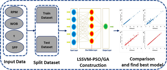
The process flow chart for calculating and forecasting ROP from one oil field in southwest Iran is shown schematically in Figure 1. This diagram illustrates how the data are initially observed from three wells. The data were collected, normalized using eq 1, and then split into two groups: the training set (80%) and the test set (20%). The LSSVM-PSO/GA hybrid algorithms were then built using the segregated data for the train data, and the test data were used to test the algorithms using empirical equations. In this paper, the k-fold cross validation was employed to prevent overfitting.
| 3 |
Figure 1.
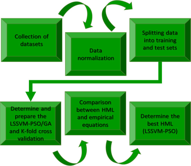
Flow chart schematic for the prediction of ROP based on LSSVM-PSO/GA.
2.2. Least Squares Support Vector Machine
This method can solve non-linear problems by taking them into multi-dimensional space and solving them through kernel functions.39,40 Additionally, due to the SVM’s high performance in function estimation, the use of this technique can be a substantial improvement in the field of modeling hydrocarbon reservoirs.41−43 The simplified relationship used in the support vector machine is expressed as eq 4(41)
| 4 |
whereas a non-linear function [(x)] converts the input variables through a multidimensional space, reducing complexity, and accelerating the solution of problems. W is the weight vector, while b is the bias value. It has the same dimension as the defined space dimension.44Equation 5 represents the parameters that are determined using linear regression44
| 5 |
where ei is the model error and is the systematic parameter. Equation 5 was introduced by Suykens et al. (2002), and it has been debated in related scientific domains.45,46 After including Mercer’s theory, eq 6 represents the least squares support vector machine (LSSVM) equation (from eq 4)45,46
| 6 |
(x,xi) is called kernel function (kernel), and it has different types, for example, linear, polynomial, radial function, and multilayers.45,47,48Table 1 shows the most common kernel functions and their mathematical expressions.45,47,48
Table 1. Common Mathematical Functions Related to LSSVM.
| core method | mathematical statement | |
|---|---|---|
| linear | K(x,xi) = xTixi + c | |
| radial (RBF) |
2.3. Particle Swarm Optimization Algorithm
This strategy, which belongs to the category of random optimization techniques, is based on the behavioral model of a group of particular species of animals, especially birds and fish.49 Previous work shows that this method works at an acceptable speed, unlike other optimization methods.50 Another reason for using particle swarm optimization (PSO) is that it requires fewer parameters to adjust. Also, its formula is simple and easy to implement.51 The formula for this method is expressed as eqs 7 and 8(51)
| 7 |
| 8 |
where V velocity of particles, r1 and r2, are two random numbers created in the interval [0,1].
1c (self-confidence) and 2c (crowd confidence) are, respectively, gbest and pbest intensities of attraction; Δt is the time parameter, which is the step of particle progress; and W is the inertial factor that manages the speed effect. The value 1 is used for w in this work.52
Collections of generated arbitrary solutions, called “particles” fly in the large space of the problem. According to the alternative equations, the position of each particle changes according to its experience (gbest) and its neighbors (pbest).
2.4. Genetic Algorithm
The genetic algorithm (GA) is an effective domain-independent search technique that was motivated by Darwin’s idea.53 Because the GA is population-based, a different answer is produced in each iteration.54 The main concept of this natural selection algorithm is that stronger people survive and pass on their strong characteristics to their children.55 This algorithm has two genetic operators: integration and mutation.56 One mechanism for kids to inherit their parents’ traits is through the genetic operator known as integration.57 The mutation of an operator is based on probabilities that happen to some people in society. The mutation introduces new characteristics to the population that they did not inherit from their parents.
2.5. Hybrid LSSVM-PSO/GA
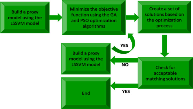
In order to reduce the simulation process and increase its performance, the initial model was replaced by a proxy model based on LSSVM.58 It took several iterations of the proxy to produce a useable model. The model was examined using GA and PSO techniques to identify the best solution. Despite the fact that the core concepts of these algorithms are fundamentally different, it was selected to apply the same requirements to both approaches. Moreover, it is required to specify an objective function to discover a suitable matching solution. In other words, after running the simulator model, the oil production rate and two pressure parameters are the outputs of the simulator model used to generate the objective function. Usually, the objective functions can be defined in different ways depending on the modeling conditions (Figure 2).
Figure 2.
Workflow for performing “automatic history matching” with the optimized alternative model of the simulator.
Three important parts are considered to define the objective function in this study, which is based on the error function.
The first stage: considering the amount of error resulting from the change of parameters on the response variables in different time intervals in each studied well, which is normalized, the difference between the response data values calculated from the proxy model and the observed (real) response data is shown as eq 9 (AResp).59 The outcome of each well’s error is taken into consideration in the second phase, as shown in eq 10 (Bwell), and the field’s overall error is then calculated by dividing the weight of each well by one, as shown in eq 11 (Ctotal).60 Finally, the objective function is briefly given as eq 12.60
| 9 |
| 10 |
| 11 |
| 12 |
The main parameters of this study, including response variables, number of wells, time intervals, and the difference between the response data calculated from the proxy model and the real model, as well as the deviation from the standard, are defined in the objective function (eq 12). In other words, the objective function value is the average percentage. Additionally, there is no zero-observation data when employing this objective function. Based on this objective function, the proxy model and optimization procedure were built.
2.6. Determining the Parameters of the Optimizer Algorithm
For the validation of the proxy model, five criteria were considered: mean square error (MSE), organizing parameter (γ), kernel width parameter (σ2), mean absolute error, and R2.61 These parameters are taken into account when comparing the calculated values to the actual values.62 If the proxy’s quality is determined to be appropriate, it can be made ready for usage after validation. The procedure will then be carried out once more to improve the proxy’s quality in such a situation. The constructed proxy model’s parameters and errors are displayed in Table 2.
Table 2. Proxy Model’s Parameter Based on the Train and Test Errors.
| Data | γ | σ2 | RMSE | R2 |
|---|---|---|---|---|
| train data | 0.95 × 10⁵ | 0.99 × 10⁷ | 0.025 | 0.9 |
| test data | 0.026 | 0.88 |
Based on the calculated error, they are compared with each other, and the parameters corresponding to the minimum error are introduced as adjustment parameters.63 The parameter checks and selection of the best parameter based on the estimated error are carried out indefinitely through change tests.64 The results of this investigation showed that the PSO algorithm performed best when the two key parameters were 1.5 and 2, respectively. The values of 0.8 and 0.2 were used for optimization, and Table 3 shows the characteristics and parameters used in both algorithms (using the trial-and-error method).
Table 3. GA and PSO’s Control Parameters.
| PSO |
GA |
||
|---|---|---|---|
| parameters | value | parameters | value |
| population | 300 | population | 300 |
| number of parameters | 44 | number of parameters | 44 |
| C1 (personal education coefficient) | 1.7 | mutation factor | 0.2 |
| C2 (global education coefficient) | 2.3 | crossover factor | 0.8 |
| W (coefficient of inertia) | 0.4 | ||
| V (maximum speed value) | 2.2 | ||
Based on the result, higher values of γ mean better performance. In other words, the parameter γ determines the trade-off between minimizing the training error and minimizing the complexity of the model. The σ2 parameter is the bandwidth and defines the non-linear mapping from the input space to a high-dimensional feature space. A high value of σ2 can make the model more economical, and a low value can make the result unfavorable.
3. Data Gathering
This article uses information about an oil well drilled into carbonate formations located in one of the southwestern regions of Iran. To predict the amount of ROP related to this field, information from 2026 drilling data was used. The drilling information includes RPM, rotation of the axis, WOB, force on the bit, torque, twisting force of the expression of drill, standpipe pressure, and loss of the total pressure (the statistical parameter shown in Table 4). These data contain a lot of noise, but by using the methods described in this article, it was possible to improve the accuracy of the performance significantly.
Table 4. Data Analysis for One of the Wells Located in the Southwest of Iran.
| parameters | RPM | WOB | τ | SPP | ROP |
| unit | rpm | klb | klbf ft | psi | m/h |
| mean | 112.4 | 6.3 | 4.0 | 721.7 | 5.7 |
| std. deviation | 21.7 | 3.5 | 3.1 | 232.5 | 2.9 |
| variance | 524.4 | 22.0 | 10.9 | 52,293.8 | 5.4 |
| minimum | 35.09 | 0.12 | 0.01 | 14.32 | 1.5 |
| maximum | 157.2 | 16.6 | 9.5 | 1101.7 | 32.8 |
| skewness | –0.4 | 0.6 | 0.1 | –1.6 | 3.2 |
| kurtosis | –0.5 | 0.3 | –1.3 | 1.3 | 18.8 |
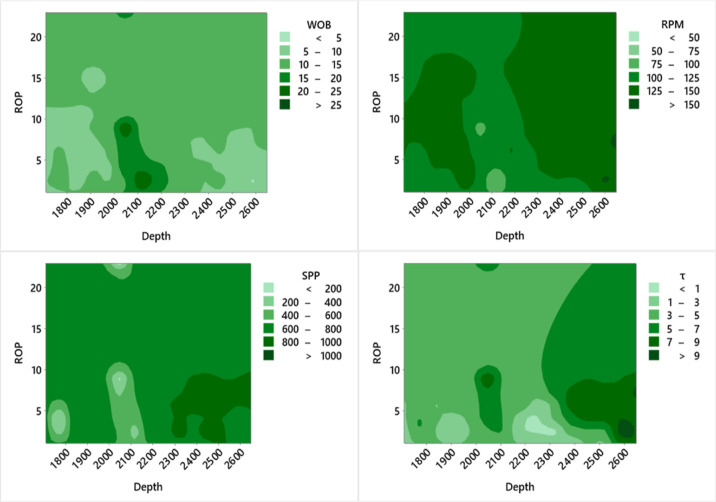
Figure 3 displays details about the parameters that were used as inputs and outputs for the data analysis applied in this research. As shown in Figure 3, only a small portion of the data is in the range of WOB > 25, and the majority of the data related to this parameter is in the range of 10–15. For the maximum RPM parameter, the data are divided into two sections: 100–125 and 125–150. For SPP data, most data are in the range of 600–800. For data related to 1, most data are between 3 and 5.
Figure 3.
Illustration of data analyses for input variables based on the depth and output variable.
4. Results and Discussion
The entire data set used in this article includes 2026 drilling data. To build artificial intelligence hybrid hearts, 80% of this data has been used for training, and the other 20% of data points have been used for testing. Hybrid artificial intelligence models have been compared with two empirical equations. To avoid overfitting, cross validation is used. To compare these common methods for determining ROP as well as artificial intelligence models, common statistical parameters have been used in the articles. Among these parameters, we can mention RMSE and R2, which are suitable for comparison (shown in eqs 13 and 14). Table 5 presents information and reports comparing artificial intelligence algorithms and empirical equations.
| 13 |
 |
14 |
Table 5. Results of the Most Relevant Test and Total Data That Were Utilized to Predict ROP Using Statistical Correctness Criteria.
| split data | models | RMSE | R2 |
|---|---|---|---|
| train data set | Maurer | 17.43 | 0.6678 |
| Galle and Woods | 20.68 | 0.5832 | |
| LSSVM | 6.19 | 0.8662 | |
| LSSVM-GA | 3.55 | 0.9018 | |
| LSSVM-PSO | 1.05 | 0.9845 | |
| test data set | Maurer | 18.29 | 0.6321 |
| Galle and Woods | 22.46 | 0.5509 | |
| LSSVM | 7.21 | 0.8034 | |
| LSSVM-GA | 4.70 | 0.8997 | |
| LSSVM-PSO | 1.92 | 0.9516 | |
| total data set | Maurer | 17.86 | 0.6500 |
| Galle and Woods | 21.57 | 0.5671 | |
| LSSVM | 6.70 | 0.8348 | |
| LSSVM-GA | 4.125 | 0.9008 | |
| LSSVM-PSO | 1.485 | 0.9681 |
The present study employed a training data set comprising 80% of the total data, while the other 20% was allocated for the purpose of testing. Based on the information reported in Table 5 (the most relevant information, test, and total data), a correct comparison can be made between empirical and hybrid models. As can be observed from the findings, the outcomes for the LSSVM-PSO hybrid model are RMSE = 1.05, R2 = 0.9845; RMSE = 1.92, R2 = 0.9516; and RMSE = 1.485, R2 = 0.9681 for the most, test, and total data. Therefore, it can be concluded that the performance accuracy of the LSSVM-PSO algorithm is better than other algorithms and empirical models.
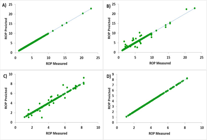
Figures 4 and 5, respectively, show the cross-plot shape for calculating the predicted and measured values of the best LSSVM-PSO algorithm, as well as the calculation of the RMSE and R2 error values. Figure 4 indicates that it has a high level of performance accuracy, and Figure 5 shows that the RMSE and R2 for the LSSVM-PSO algorithm have a greater level of performance accuracy.
Figure 4.
Illustration of cross-plot chart for predicted ROP and measured ROP for comparison of LSSVM and LSSVM-PSO algorithms.
Figure 5.
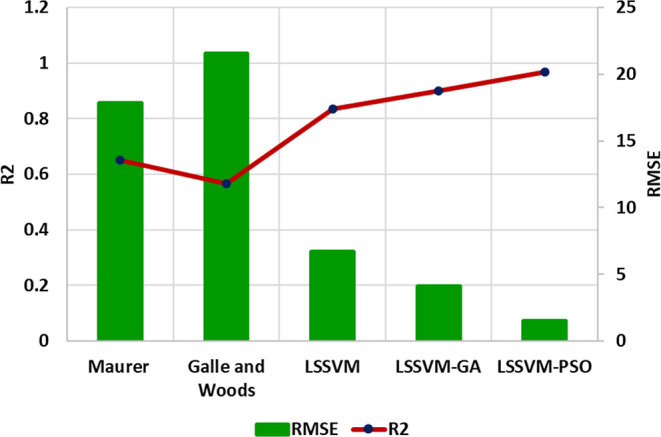
Determination of the RMSE and R2 values based on the statistical metric.
The value of R2 increases with an increase in RMSE, which is one of the conclusions that can be drawn from this graph and is one of the greatest metrics for comparing models.
According to the results presented in Figure 5, the following can be concluded:
RMSE: Galle and Woods > Maurer > LSSVM-GA > LSSVM-PSO.
R2: Galle and Woods < Maurer < LSSVM-GA < LSSVM-PSO.
Upon analysis of the findings presented in Figure 6, which pertain to each iteration of both hybrid models, namely, LSSVM-PSO/GA, it is evident that the LSSVM-PSO algorithm exhibits convergence for both the input and predicted data and outperforms the LSSVM-GA algorithm. As can be seen, for the LSSVM-PSO algorithm, in the beginning, in iterations between 1 and 50, this algorithm initially has a lower performance accuracy. Still, this convergence in iteration 50 is much higher than LSSVM-GA. The findings of this study suggest that the algorithm presented herein can be utilized by researchers to forecast not only the aforementioned issue but also other significant parameters related to all petro-science.
Figure 6.
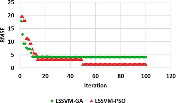
Determination of Iteration for two hybrid models and comparing them.
5. Limitations
The lack of total continuity in well logs is one of the factors that makes predicting well logs difficult; nevertheless, in this study, drilling logs had continuing logs. However, there are certain limits to this article, such as the fact that the data occasionally contains outliers. We were able to investigate this issue and eliminate the outlier data by using the outlier identification approach.
6. Conclusions and Recommendation
In this article, rotation speed, rotation of the axis, WOB, force on the bit, torque, twisting force of the expression of drill, standpipe pressure, and loss of the total pressure have been used to predict ROP. In this article, 2026 drilling data points from one of the southwestern Iran wells were used. This article used two combined methods, LSSVM-PSO and LSSVM-GA, and empirical equations to predict the ROP. Using PSO and GA optimizers improves performance accuracy and correctly determines control parameters. Upon analysis of the findings, it is evident that the LSSVM-PSO algorithm exhibits superior performance accuracy compared to the other algorithms and equations. For test data of the LSSVM-PSO algorithm with high accuracy, RMSE = 1.92 and R2 = 0.9516. For the prevention of overfitting the data, we used the cross-validation method.
The accuracy of the LSSVM-PSO model also improves and degrades after the 50th iteration according to our analysis of the two algorithms. Even so, following the 10th iteration of the LSSVM-GA algorithm, these modifications are still consistent. One of the advantages of these two algorithms is that they decrease the data noise for drilling data. One of the LSSVM algorithm’s features is its high accuracy and high-performance time. Based on the results, it is revealed that researchers can use this algorithm to predict this issue or even other key parameters for reservoirs, production, drilling, and geophysics.
Glossary
Nomenclature
- b
bias value
- db
drill bit diameter
- K
proportionality constant
- M
number of wells R
- N
number of response variables
- P
number of time steps
- R2
R-square
- RMSE
root mean square error
- ROP
rate of penetration
- RPM
rotation speed
- S
rock strength
- STD
standard deviation
- W
weight
- WOB
weight on bit
- Wt
threshold bit
- Yo
objective function defined for time intervals
- V
velocity of particles
- Wwell–i and Wresponses
weighting factors for wells and responses
- Yhis
observational response data (real)
- Ycalc
response data calculated from the proxy model
- (x,)
Kernel function
- Δt
time parameter
- γ
systematic parameter
- δli
normalize variable
- δmax
maximum variable
- δmin
minimum variable
- ei
error
- (x)
non-linear function
Author Contributions
Conceptualization, S.V.A.N.K.A., O.H., H.G., A.E.R., and M.M.; writing—original draft, M.R., S.T., S.L., and H.G.; methodology, S.L., H.G., S.T., M.M., M.R., and A.E.R; resources, H.G. and A.E.R; visualization, M.M., H.G., and M.R; writing—review and editing, S.T., H.G., S.L., and M.R; and funding acquisition, O.H., H.G., and M.R. All authors have read and agreed to the published version of the manuscript.
The authors declare no competing financial interest.
Notes
The corresponding authors can make data available upon reasonable requests for academic purposes.
References
- Bello O.; Holzmann J.; Yaqoob T.; Teodoriu C. Application of artificial intelligence methods in drilling system design and operations: a review of the state of the art. J. Artif. Intell. Soft Comput. Res. 2015, 5, 121–139. 10.1515/jaiscr-2015-0024. [DOI] [Google Scholar]
- Hassanpouryouzband A.; Joonaki E.; Edlmann K.; Haszeldine R. S. Offshore geological storage of hydrogen: Is this our best option to achieve net-zero?. ACS Energy Letters 2021, 6, 2181–2186. 10.1021/acsenergylett.1c00845. [DOI] [Google Scholar]
- Radwan A. E. Drilling in Complex Pore Pressure Regimes: Analysis of Wellbore Stability Applying the Depth of Failure Approach. Energies 2022, 15, 7872. 10.3390/en15217872. [DOI] [Google Scholar]
- Schultz R. A.; Williams-Stroud S.; Horváth B.; Wickens J.; Bernhardt H.; Cao W.; Capuano P.; Dewers T. A.; Goswick R. A.; Lei Q.; et al. Underground energy-related product storage and sequestration: site characterization, risk analysis, and monitoring. Geological Society 2023, 528, SP528-2022-66. 10.1144/sp528-2022-66. [DOI] [Google Scholar]
- Huang L.; Liu J.; Zhang F.; Dontsov E.; Damjanac B. Exploring the influence of rock inherent heterogeneity and grain size on hydraulic fracturing using discrete element modeling. Int. J. Solids Struct. 2019, 176–177, 207–220. 10.1016/j.ijsolstr.2019.06.018. [DOI] [Google Scholar]
- Li M.; Jian Z.; Hassanpouryouzband A.; Zhang L. Understanding Hysteresis and Gas Trapping in Dissociating Hydrate-Bearing Sediments Using Pore Network Modeling and Three-Dimensional Imaging. Energy Fuels 2022, 36, 10572–10582. 10.1021/acs.energyfuels.2c01306. [DOI] [Google Scholar]
- Marbun B.; Aristya R.; Pinem R. H.; Ramli B. S.; Gadi K. B.. Evaluation of non productive time of geothermal drilling operations–case study in Indonesia, 2013, 2013.
- Ponomareva I. N.; Galkin V. I.; Martyushev D. A. Operational method for determining bottom hole pressure in mechanized oil producing wells, based on the application of multivariate regression analysis. Pet. Res. 2021, 6, 351–360. 10.1016/j.ptlrs.2021.05.010. [DOI] [Google Scholar]
- Ponomareva I. N.; Martyushev D. A.; Kumar Govindarajan S. A new approach to predict the formation pressure using multiple regression analysis: Case study from Sukharev oil field reservoir–Russia. J. Eng. Sci. King Saud Univ. 2022, 10.1016/j.jksues.2022.03.005. [DOI] [Google Scholar]
- Tan P.; Pang H.; Zhang R.; Jin Y.; Zhou Y.; Kao J.; Fan M. Experimental investigation into hydraulic fracture geometry and proppant migration characteristics for southeastern Sichuan deep shale reservoirs. J. Petrol. Sci. Eng. 2020, 184, 106517. 10.1016/j.petrol.2019.106517. [DOI] [Google Scholar]
- Teodoriu C.; Bello O. An Outlook of Drilling Technologies and Innovations: Present Status and Future Trends. Energies 2021, 14, 4499. 10.3390/en14154499. [DOI] [Google Scholar]
- Galkin V. I.; Ponomareva I. N.; Martyushev D. A. Prediction of reservoir pressure and study of its behavior in the development of oil fields based on the construction of multilevel multidimensional probabilistic-statistical models. Gas 2021, 23, 73–82. 10.18599/grs.2021.3.10. [DOI] [Google Scholar]
- Langella A.; Nele L.; Maio A. A torque and thrust prediction model for drilling of composite materials. Composites, Part A 2005, 36, 83–93. 10.1016/s1359-835x(04)00177-0. [DOI] [Google Scholar]
- Tan P.; Jin Y.; Pang H. Hydraulic fracture vertical propagation behavior in transversely isotropic layered shale formation with transition zone using XFEM-based CZM method. Eng. Fract. Mech. 2021, 248, 107707. 10.1016/j.engfracmech.2021.107707. [DOI] [Google Scholar]
- Tay F. E. H.; Cao L. J. Modified support vector machines in financial time series forecasting. Neurocomputing 2002, 48, 847–861. 10.1016/s0925-2312(01)00676-2. [DOI] [Google Scholar]
- Thaysen E. M.; Butler I. B.; Hassanpouryouzband A.; Freitas D.; Alvarez-Borges F.; Krevor S.; Heinemann N.; Atwood R.; Edlmann K. Pore-scale imaging of hydrogen displacement and trapping in porous media. Int. J. Hydrogen Energy 2023, 48, 3091–3106. 10.1016/j.ijhydene.2022.10.153. [DOI] [Google Scholar]
- Wang Y.; Salehi S. Application of real-time field data to optimize drilling hydraulics using neural network approach. J. Energy Resour. Technol. 2015, 137, 062903. 10.1115/1.4030847. [DOI] [Google Scholar]
- Barrett P. J. The shape of rock particles, a critical review. Sedimentology 1980, 27, 291–303. 10.1111/j.1365-3091.1980.tb01179.x. [DOI] [Google Scholar]
- DeJong J. T.; Jaeger R. A.; Boulanger R. W.; Randolph M. F.; Wahl D. A. J.. Variable penetration rate cone testing for characterization of intermediate soils. Geotechnical and Geophysical Site Characterization, 2012; Vol. 4( (1), ) pp 25–42.
- Purba D.; Adityatama D. W.; Agustino V.; Fininda F.; Alamsyah D.; Muhammad F.. Geothermal drilling cost optimization in Indonesia: a discussion of various factors, 2020, 2020.
- Boyou N. V.; Ismail I.; Wan Sulaiman W. R.; Sharifi Haddad A.; Husein N.; Hui H. T.; Nadaraja K. Experimental investigation of hole cleaning in directional drilling by using nano-enhanced water-based drilling fluids. J. Petrol. Sci. Eng. 2019, 176, 220–231. 10.1016/j.petrol.2019.01.063. [DOI] [Google Scholar]
- Martyushev D. A.; Ponomareva I. N.; Filippov E. V. Studying the direction of hydraulic fracture in carbonate reservoirs: Using machine learning to determine reservoir pressure. Pet. Res. 2023, 8, 226–233. 10.1016/j.ptlrs.2022.06.003. [DOI] [Google Scholar]
- Zakharov L. A.Application of machine learning for forecasting formation pressure in oil field development. Proceedings of the Tomsk Polytechnic University Geo Assets Engineering, 2021; p 148.
- Dupriest F. E.; Koederitz W. L.. Maximizing drill rates with real-time surveillance of mechanical specific energy, 2005; OnePetro, 2005.
- Kurt M.; Kaynak Y.; Bagci E. Evaluation of drilled hole quality in Al 2024 alloy. Int. J. Adv. Des. Manuf. Technol. 2008, 37, 1051–1060. 10.1007/s00170-007-1049-1. [DOI] [Google Scholar]
- Tewari S.; Dwivedi U. D.; Biswas S. A novel application of ensemble methods with data resampling techniques for drill bit selection in the oil and gas industry. Energies 2021, 14, 432. 10.3390/en14020432. [DOI] [Google Scholar]
- Bourgoyne A. T.; Young F. S. A multiple regression approach to optimal drilling and abnormal pressure detection. Soc. Petrol. Eng. J. 1974, 14, 371–384. 10.2118/4238-pa. [DOI] [Google Scholar]
- Li J.; Walker S.. Sensitivity analysis of hole cleaning parameters in directional wells. In SPE/ICoTA Well Intervention Conference and Exhibition, pp. SPE-54498-MS, 1999 10.2118/54498-MS. [DOI]
- Hegde C.; Gray K. Evaluation of coupled machine learning models for drilling optimization. J. Nat. Gas Sci. Eng. 2018, 56, 397–407. 10.1016/j.jngse.2018.06.006. [DOI] [Google Scholar]
- Graham J. W.; Muench N. L.. Analytical determination of optimum bit weight and rotary speed combinations, 1959; OnePetro, 1959.
- Maurer W. C. The perfect-cleaning theory of rotary drilling. J. Petrol. Technol. 1962, 14, 1270–1274. 10.2118/408-pa. [DOI] [Google Scholar]
- Galle E. M.; Woods H. B.. Best Constant Weight and Potary Speed For Rotary Rock Bits; Hughes Tool Co., 1963. [Google Scholar]
- Yang J.-F.; Zhai Y.-J.; Xu D.-P.; Han P.. SMO algorithm applied in time series model building and forecast, 2007; IEEE, 2007; pp 2395-2400.
- Elkatatny S.; Tariq Z.; Mahmoud M. Real time prediction of drilling fluid rheological properties using Artificial Neural Networks visible mathematical model (white box). J. Petrol. Sci. Eng. 2016, 146, 1202–1210. 10.1016/j.petrol.2016.08.021. [DOI] [Google Scholar]
- Salahdin O. D.; Salih S. M.; Jalil A. T.; Aravindhan S.; Abdulkadhm M. M.; Huang H. Current challenges in seismic drilling operations: a new perspective for petroleum industries. Asian J. Water Environ. Pollut. 2022, 19, 69–74. 10.3233/ajw220041. [DOI] [Google Scholar]
- Bataee M.; Mohseni S.. Application of Artificial Intelligent Systems in ROP Optimization: A Case Study in Shadegan Oil Field, 2011; OnePetro, 2011.
- Jahanbakhshi R.; Keshavarzi R.; Jafarnezhad A.. Real-Time Prediction of Rate of Penetration During Drilling Operation in Oil and Gas Wells, 2012; OnePetro, 2012.
- Elkatatny S. Development of a new rate of penetration model using self-adaptive differential evolution-artificial neural network. Arabian J. Geosci. 2019, 12, 19. 10.1007/s12517-018-4185-z. [DOI] [Google Scholar]
- Zhao Y.; Noorbakhsh A.; Koopialipoor M.; Azizi A.; Tahir M. M. A new methodology for optimization and prediction of rate of penetration during drilling operations. Eng. Comput. 2020, 36, 587–595. 10.1007/s00366-019-00715-2. [DOI] [Google Scholar]
- Chen J.-S.; Pan C.; Wu C.-T.; Liu W. K. Reproducing kernel particle methods for large deformation analysis of non-linear structures. Comput. Methods Appl. Mech. Eng. 1996, 139, 195–227. 10.1016/s0045-7825(96)01083-3. [DOI] [Google Scholar]
- Patil N. S.; Shelokar P. S.; Jayaraman V. K.; Kulkarni B. D. Regression models using pattern search assisted least square support vector machines. Chem. Eng. Res. Des. 2005, 83, 1030–1037. 10.1205/cherd.03144. [DOI] [Google Scholar]
- Shamshirband S.; Mosavi A.; Rabczuk T.; Nabipour N.; Chau K.-w. Prediction of significant wave height; comparison between nested grid numerical model, and machine learning models of artificial neural networks, extreme learning and support vector machines. Eng. Appl. Comput. Fluid Mech. 2020, 14, 805–817. 10.1080/19942060.2020.1773932. [DOI] [Google Scholar]
- Otchere D. A.; Arbi Ganat T. O.; Gholami R.; Ridha S. Application of supervised machine learning paradigms in the prediction of petroleum reservoir properties: Comparative analysis of ANN and SVM models. J. Petrol. Sci. Eng. 2021, 200, 108182. 10.1016/j.petrol.2020.108182. [DOI] [Google Scholar]
- Wang S.; Chen S. Insights to fracture stimulation design in unconventional reservoirs based on machine learning modeling. J. Petrol. Sci. Eng. 2019, 174, 682–695. 10.1016/j.petrol.2018.11.076. [DOI] [Google Scholar]
- Zhang G.; Band S. S.; Jun C.; Bateni S. M.; Chuang H.-M.; Turabieh H.; Mafarja M.; Mosavi A.; Moslehpour M. Solar radiation estimation in different climates with meteorological variables using Bayesian model averaging and new soft computing models. Energy Rep. 2021, 7, 8973–8996. 10.1016/j.egyr.2021.10.117. [DOI] [Google Scholar]
- Suykens J. A. K.; Vandewalle J.; De Moor B. Optimal control by least squares support vector machines. Neural Network. 2001, 14, 23–35. 10.1016/s0893-6080(00)00077-0. [DOI] [PubMed] [Google Scholar]
- Tavoosi J.; Mohammadzadeh A.; Pahlevanzadeh B.; Kasmani M. B.; Band S. S.; Safdar R.; Mosavi A. H. A machine learning approach for active/reactive power control of grid-connected doubly-fed induction generators. Ain Shams Eng. J. 2022, 13, 101564. 10.1016/j.asej.2021.08.007. [DOI] [Google Scholar]
- Adankon M. M.; Cheriet M.; Biem A. Semisupervised least squares support vector machine. IEEE Trans. Neural Network. 2009, 20, 1858–1870. 10.1109/tnn.2009.2031143. [DOI] [PubMed] [Google Scholar]
- Samadianfard S.; Jarhan S.; Salwana E.; Mosavi A.; Shamshirband S.; Akib S. Support vector regression integrated with fruit fly optimization algorithm for river flow forecasting in Lake Urmia Basin. Water 2019, 11, 1934. 10.3390/w11091934. [DOI] [Google Scholar]
- Dilmac S.; Korurek M. ECG heart beat classification method based on modified ABC algorithm. Appl. Soft Comput. 2015, 36, 641–655. 10.1016/j.asoc.2015.07.010. [DOI] [Google Scholar]
- Haji S. H.; Abdulazeez A. M. Comparison of optimization techniques based on gradient descent algorithm: A review. PalArch’s J. Archaeol. 2021, 18, 2715–2743. [Google Scholar]
- Pedersen M. E. H.; Chipperfield A. J. Simplifying particle swarm optimization. Appl. Soft Comput. 2010, 10, 618–628. 10.1016/j.asoc.2009.08.029. [DOI] [Google Scholar]
- Kennedy J.; Eberhart R.. Particle swarm optimization, 1995; IEEE, 1995; pp 1942-1948.
- Krouska A.; Troussas C.; Sgouropoulou C. A novel group recommender system for domain-independent decision support customizing a grouping genetic algorithm. User Model. User-Adapted Interact. 2023, 10.1007/s11257-023-09360-3. [DOI] [Google Scholar]
- Fallah M. K.; Fazlali M.; Daneshtalab M. A symbiosis between population based incremental learning and LP-relaxation based parallel genetic algorithm for solving integer linear programming models. Computing 2021, 105, 1121–1139. 10.1007/s00607-021-01004-x. [DOI] [Google Scholar]
- Geraedts C. L.; Boersma K. T. Reinventing natural selection. Int. J. Environ. Sci. Educ. 2006, 28, 843–870. 10.1080/09500690500404722. [DOI] [Google Scholar]
- Nguyen H. B.; Xue B.; Andreae P.; Zhang M.. Particle swarm optimisation with genetic operators for feature selection; IEEE, 2017; pp 286–293.
- Kumar M.; Husain D.; Upreti N.; Gupta D.. Genetic algorithm: Review and application. Available at SSRN 3529843 2010.
- Karimi M. A new approach to history matching based on feature selection and optimized least square support vector machine. J. Geophys. Eng. 2018, 15, 2378–2387. 10.1088/1742-2140/aad1c8. [DOI] [Google Scholar]
- Hausman J. A.; Abrevaya J.; Scott-Morton F. M. Misclassification of the dependent variable in a discrete-response setting. J. Econom. 1998, 87, 239–269. 10.1016/s0304-4076(98)00015-3. [DOI] [Google Scholar]
- Zipper S. C.; Gleeson T.; Kerr B.; Howard J. K.; Rohde M. M.; Carah J.; Zimmerman J. Rapid and accurate estimates of streamflow depletion caused by groundwater pumping using analytical depletion functions. Water Resour. Res. 2019, 55, 5807–5829. 10.1029/2018wr024403. [DOI] [Google Scholar]
- Gala Y.; Fernández Á.; Díaz J.; Dorronsoro J. R. Hybrid machine learning forecasting of solar radiation values. Neurocomputing 2016, 176, 48–59. 10.1016/j.neucom.2015.02.078. [DOI] [Google Scholar]
- Wang L.; Yao Y.; Wang K.; Adenutsi C. D.; Zhao G.; Lai F. Hybrid application of unsupervised and supervised learning in forecasting absolute open flow potential for shale gas reservoirs. Energy 2022, 243, 122747. 10.1016/j.energy.2021.122747. [DOI] [Google Scholar]
- Brezinski C.; Rodriguez G.; Seatzu S. Error estimates for the regularization of least squares problems. Numer. Algorithm. 2009, 51, 61–76. 10.1007/s11075-008-9243-2. [DOI] [Google Scholar]
- De Kruif B. J.; De Vries T. J. A. Pruning error minimization in least squares support vector machines. IEEE Trans. Neural Network. 2003, 14, 696–702. 10.1109/tnn.2003.810597. [DOI] [PubMed] [Google Scholar]


