The context dependency of fish‐habitat associations in separated karst ecoregions

Abstract

Fish populations may be isolated via natural conditions in geographically separated ecoregions. Although reconnecting these populations is not a management goal, we need to understand how these populations persist across landscapes to develop meaningful conservation actions, particularly for species occupying sensitive karst ecosystems. Our study objective was to determine the physicochemical factors related to the occurrence of four spring‐associated fishes. Arbuckle Uplift and Ozark Highlands ecoregions, USA. We used a hierarchical approach to identify habitat relationships at multiple spatial scales. We collected detection data using snorkeling and seining. We examined the physicochemical relationships related to the detection and occurrence of four spring‐associated fishes using occupancy modeling in a Bayesian framework. We found physicochemical relationships that differed and were similar between ecoregions for several fishes. For three species, we found different water temperature relationships between ecoregions. Smallmouth bass were ubiquitous in their use of drainage areas in the Ozark Highlands but only associated with the lower network of the Arbuckle Uplift. There were several mirrored relationships between ecoregions, including an interaction between residual pool depth and water temperature, where sites with deeper pools were more likely to be occupied during warmer water temperatures. There were single‐species occurrence relationships with percent vegetation and percent agriculture. Lastly, snorkeling was a more efficient sampling method compared to seining for all fishes. Our results indicate stream temperature mitigation may be possible via the maintenance of key channel morphologies, and we identify shared stressors between ecoregions. Channel mitigation to maintain reaches with deeper pools may be an important strategy for maintaining thermal refugia, particularly when considering climate change. Identifying the mechanistic underpinning of other multiscale ecological relationships would be helpful to discern if some of the different ecoregion relationships represent warning signals or interactions with unmeasured biotic or abiotic factors.

Fish populations may be isolated via natural conditions in geographically separated ecoregions. Although reconnecting these populations is not a management goal, we do need to understand how these populations persist across different landscapes to develop meaningful conservation actions, particularly for species occupying sensitive karst ecosystems. Our study objective was to determine the physicochemical factors related to the occurrence of four spring‐associated fishes.

1. INTRODUCTION

Populations within broader species distributions can become isolated by natural phenomena; thus, their distributions may be related to different physicochemical conditions depending on the surrounding landscape. Natural features that isolate populations include glacial movements (Berendzen et al., 2010), stream capture (Buth & Mayden, 1981), and tectonic lifts (McKeown et al., 1988). For example, many fishes in the Ozark Highlands and Great Plains ecoregions appear to have recolonized northern areas of the range from a southern Ozark Highland refuge (e.g., carmine shiner Notropis percobromus, Berendzen et al., 2008). Distribution information on populations is useful for a variety of conservation and management needs including identifying habitat refugia over time (Lake, 2000; Magoulick & Kobza, 2003; Peterson & Rabeni, 1996; Torgersen et al., 1999), identifying locations to manage with limited resources (Dauwalter & Rahel, 2008; Gardner et al., 2013; Gore et al., 2001; Park et al., 2003; Rabeni & Sowa, 1996; Wilson et al., 2005), determining species conservation status (e.g., goldline darter Percina aurolineata, Albanese et al., 2004; Potoka et al., 2016), and identifying areas of reintroduction (Bearlin et al., 2002; Wall et al., 2004). Reconnecting naturally isolated populations is not a management goal; however, understanding how these populations persist across different landscapes is helpful to developing meaningful conservation and management actions (i.e., are the populations limited by different physicochemical conditions?).

The distribution of stream fauna is related to physicochemical relationships at multiple spatial scales (Hynes, 1975; Poff et al., 1997; Vannote et al., 1980). Coarse‐scale distributions of stream fishes are constrained primarily by factors that change relatively slowly such as climate and geology (Hynes, 1975; Marsh‐Matthews & Matthews, 2000). However, a myriad of physicochemical factors determines stream fish distributions at finer spatial scales (e.g., segments, reaches, and microhabitats, Goldstein & Meador, 2004; Poff et al., 1997; Southwood, 1977; Vannote et al., 1980). For example, groundwater (Brewer, 2013a; Power et al., 1999) and water temperature (Constantz, 1998; Last et al., 2011; Wehrly et al., 2006; Wolf et al., 2019) affect habitat selection by stream fishes at different spatial scales (e.g., patch or reach) and seasonally. Viewing stream fauna and their relationships with physicochemical factors at a single scale can lead to erroneous conclusions (Dunham & Vinyard, 1997). For example, pool habitat is important to smallmouth bass Micropterus dolomieu at a fine scale (Brewer, 2013b), but the abundance of smallmouth bass declines when pool habitat area increases at the reach scale (Brewer, 2013b). A more insightful approach is to view distributions in a hierarchical framework (Frissell et al., 1986). By viewing physicochemical relationships with fish presence in a hierarchical framework, coarse‐scale relationships can help guide conservation practices across the riverscape (Fausch et al., 2002; Rabeni & Sowa, 1996).

Groundwater creates suitable habitat patches for some species across multiple spatial scales (Brewer, 2013a). Stream reaches influenced by groundwater are important determinants of a stream's thermal regime (Caissie, 2006). Groundwater can create important thermal habitats for stream organisms (Caissie, 2006; Farless & Brewer, 2017; Glazier, 1991; Hubbs, 1995). These habitats often have different water chemistry, temperature, and ecological structure and function within the stream network (Hubbs, 1995). Spring‐associated species tend to be emblematic of karst regions (Bergey et al., 2008; Hubbs, 2001; Matthews et al., 1985); however, these species also occupy narrow spatial extents and are typically understudied (Bergey et al., 2008; Kollaus & Bonner, 2012; Matthews et al., 1985; Spitale, 2012). Groundwater species with narrow distributions (e.g., watercress darter Etheostoma nuchale, Duncan et al., 2010) or patchy distributions, (e.g., Arkansas darter Etheostoma cragini, Groce et al., 2012) often occupy locations with above‐average stream quality and provide areas of focus for conservation and management (Fausch et al., 1990). Spring‐associated species play an important ecological role as they are often the primary consumers of invertebrates (e.g., herbivorous insects, Cordes & Page, 1980) and reside in locations where insectivorous fishes are functionally very important (i.e., few piscivores, Bergey et al., 2008; Matthews et al., 1985). Although there is a general consensus that spring systems are important for a variety of biota and human ecosystem services (Biggs et al., 2017), we do not have a good understanding of the habitat needs of organisms that are endemic to springs in different ecoregions.

Our study objective was to identify the multiscale factors related to variation in occurrence among habitat patches for four spring‐associated fishes that occupy two separated ecoregions: least darter Etheostoma microperca, redspot chub Nocomis asper, southern redbelly dace Chrosomus erythogaster, age 1+ smallmouth bass and age‐0 smallmouth bass (≤85 mm total length). We examined differences in occurrence probability both across and between ecoregions. Our focal species represent emblematic assemblage members that are associated with higher groundwater flow (Brewer, 2013a; Seilheimer & Fisher, 2010). These four species have been documented to be associated with groundwater‐fed reaches in both study ecoregions. Additionally, the populations in eastern Oklahoma are the southern‐most extent of the species' native ranges where water temperature can be more important to their persistence. The critical thermal maximum of juvenile smallmouth bass is ~35°C (adult fishes; Brewer et al., 2022) and non‐spring‐fed streams in these ecoregions commonly exceed this threshold. Species associated with higher groundwater flows are more susceptible to disturbances because of the limited available habitat. Groundwater sources can easily become polluted or extracted to the point where they no longer create thermally unique patches (Matthews et al., 1985). Smallmouth bass is also the top‐level predator in smaller streams and these streams are important habitats for age‐0 survival (Miller & Brewer, 2021) and growth in our study ecoregions (Brewer, 2013a; Brewer & Orth, 2014).

2. METHODS

2.1. Study area

We sampled fishes and instream habitats in both the Ozark Highlands (level‐3, United States Environmental Protection Agency, 2017) and Arbuckle Uplift (level‐4, United States Environmental Protection Agency, 2017) ecoregions (hereafter ecoregion, Figure 1). The Ozark Highlands ecoregion encompasses portions of northeast Oklahoma, southern Missouri, southeast Kansas, and northern Arkansas, USA. The ecoregion is relatively humid (102–122 cm precipitation annually, Woods et al., 2005), limestone dominated, and comprises mixed deciduous forest with lowland grassland and pasture areas (Woods et al., 2005). The Arbuckle Uplift rises in south‐central Oklahoma and the ecoregion receives 96–109 cm of precipitation annually. The Arbuckle Uplift is dominated by dolostone, limestone, and granite lithologies (Woods et al., 2005). Land cover comprises tallgrass prairie and oak savannas, with cropland and pasture occurring in lowland areas (Woods et al., 2005). Both ecoregions are influenced by karst topography (i.e., dissolved carbonate terrains) and spring flow characteristics (Woods et al., 2005). Springs of the Ozark Highlands vary substantially in size (Vineyard & Feder, 1982) and discharge within the stream channel or contribute to surface waters via hyporheic flow (Zhou et al., 2018). Springs of the Arbuckle Uplift ecoregion are typically isothermic (Christenson et al., 2011; Osborn, 2009) and located on small spring branches. Threats to riverine biota in both ecoregions include impoundments, land‐use practices including mining and irrigation (Christenson et al., 2011), poultry pollution (Olsen et al., 2012), altered flow patterns, degraded water quality, and accelerated streambank erosion (Woods et al., 2005).

FIGURE 1.

Reaches sampled (black circles) in summer 2018 (30 reaches) and 2019 (31 reaches) and least darter detections (black triangles) in the Arbuckle Uplift ecoregion (dark gray, Woods et al., 2005) and Ozark Highland ecoregion (light gray, Woods et al., 2005) of Oklahoma. This figure was produced using ArcGIS (10.7.1, Redlands, CA). Data layers for ecoregions (level 3 and level 4 ecoregions United States Environmental Protection Agency, https://www.epa.gov/eco‐research/level‐iii‐and‐iv‐ecoregions‐continental‐united‐states); state boundaries and counties (U.S. Department of Agriculture, Geospatial data gateway, https://datagateway.nrcs.usda.gov/GDGOrder.aspx?order=QuickState); and National Hydrography Data Plus (U.S. Environmental protection Agency, https://www.epa.gov/waterdata/get‐nhdplus‐national‐hydrography‐dataset‐plus‐data) are publicly available.

2.2. Fish sampling

At each riffle‐run‐pool complex (hereafter site, where a riffle was classified by higher gradient and a run as a transitional area between depositional pools and riffles, Rabeni & Jacobson, 1993), two temporally replicated surveys were conducted to account for imperfect gear detection (MacKenzie et al., 2002; Tyre et al., 2003). Because spring‐associated species can be patchily distributed but also locally abundant (Pflieger, 1997), we anticipated an average detection probability of .50 (the species was equally likely to be observed as not observed) when designing our study.

We used both snorkeling and seining to complete surveys during the baseflow, summer period (July–August) over 2 years (2018–2019). Two sampling approaches provided more flexibility because neither method was ideal at all sites (i.e., some were too shallow to snorkel or too deep to seine). Access locations were identified based on permission from private landowners and locations adjacent to streams. Sites (typically 100–200 m in length) were selected randomly on lands where we had access permission and sampled twice during the season, resulting in four surveys at sites where both methods were possible, to ensure heterogeneity in the detection probability estimates (Dunham et al., 2009; MacKenzie et al., 2002). We snorkeled prior to seining to prevent altering the habitat because snorkeling is minimally invasive. Snorkel surveys followed the general standardized protocol described by Dunham et al. (2009) and were conducted between 0800 hours and 1800 hours (i.e., when daylight was most conducive to sampling, Spyker & Van Den Berghe, 1995) at sites with horizontal visibility >1 m. We snorkeled all wadeable habitat in an upstream direction at approximately 2 m/min. Snorkelers walked slowly upstream and visually scanned the streambed in areas too shallow to submerge their mask completely. Depending on channel width, we used either one or two persons where snorkelers were randomly assigned to a lane (Thurow, 1994). We seined using the standardized protocol described by Rabeni et al. (2009) and used multiple seine hauls (1.5 m × 3.0 m sein with 1.5 mm mesh) to cover all applicable stream habitat.

2.3. Physicochemical conditions

We measured covariates at each site (i.e., riffle‐run‐pool complex) hypothesized to relate to stream fishes' detection (Table 1). Mean water‐column velocity (0.6 of water depth at depths <1.0 m, Gordon et al., 2004) and average water depth of each site were measured along three, evenly spaced transects perpendicular to streamflow using a Marsh McBirney Flo‐mate (Hach, Loveland, Colorado) and wading rod. Coarse substrate was estimated as a percent of the available substrate ≥90 mm diameter (Wentworth, 1922). Percent coverage of coarse wood (1.0 m², i.e., circumference > 10 cm, Dodd et al., 2008) and emergent vegetation were visually estimated at each site. Because water clarity is related to fish detection (Thurow, 1994), we measured horizontal clarity using a Secchi disk. A single value was applied to multiple sites if they occurred within the same reach because we did not observe differences in water clarity between nested sites.

TABLE 1.

Detection and occurrence of covariate summary statistics hypothesized to relate to the detection and occurrence of fish in streams.

Covariate	Arbuckle uplift mean ± SD (range)	Ozark highlands mean ± SD (range)
Detection
Coarse wood (%)	14.00 ± 13.18 (0.00–65.00)	16.00 ± 16.51 (0.00–75.00)
Coarse substrate (%)	25.00 ± 18.71 (0.00–70.00)	28.00 ± 20.40 (5.00–85.00)
Vegetation (%)	25.00 ± 29.17 (0.00–95.00)	14.00 ± 18.60 (0.00–95.00)
Water velocity (m/s)	0.17 ± 0.11 (0.00–0.47)	0.16 ± 0.13 (0.00–0.64)
Water depth (m)	0.30 ± 0.16 (0.09–0.97)	0.27 ± 0.14 (0.06–0.72)
Water clarity (m) a	2.70 ± 2.08 (0.20–11.50)	4.40 ± 1.61 (1.60–11.20)
Water temperature (°C) a	22.96 ± 3.87 (14.20–30.80)	23.84 ± 2.73 (17.00–8.80)
Occurrence
Fine substrate (%)	39.00 ± 26.65 (0.00–90.00)	10.00 ± 11.78 (0.00–85.00)
Residual pool depth (m)	0.54 ± 0.40 (0.00–1.95)	0.74 ± 0.53 (0.02–2.20)
Seepage run (m/s3)	0.02 ± 0.09 (−0.14–0.45)	0.03 ± 0.15 (−0.24–1.26)
Water temperature (°C) a	23.40 ± 3.56 (17.07–28.85)	23.15 ± 2.52 (16.14–27.77)
Drainage area (km2) a	73.65 ± 110.25 (1.00–329.08)	92.56 ± 94.9 (15.82–543.90)
Agriculture (%) a	18.31 ± 8.75 (0.01–33.57)	43.30 ± 17.14 (5.70–74.18)
Pool (%)	59.00 ± 24.00 (0.00–98.00)	0.54 ± 0.26 (0.00–96.00)
Vegetation (%)	25.00 ± 29.39 (0.00–93.00)	14.73 ± 18.63 (0.00–90.00)
Coarse wood (%)	14.00 ± 12.56 (0.00–52.00)	15.67 ± 16.13 (0.00–70.00)

Abbreviation: SD, Standard deviation.

^a Reach scale.

We quantified both site and reach covariates to determine the multiscale factors associated with species occurrence. First, the surface area (1.0 m²) of each channel unit (i.e., pool, riffle, and run) at each site was estimated by averaging wetted width at approximately three points and multiplying by the channel unit length. These values were summed for the total area of a site (m²). Additionally, we visually estimated the percent of sand and silt at each site because the least darter has been associated with finer substrates (Burr & Page, 1979). Percent coarse wood, percent vegetation, and average site velocity were quantified as previously described for detection. Residual pool depth (RPD) of each site (i.e., depth independent of discharge) was measured as described by Lisle (1987), as the difference between channel depth at the riffle crest and the deepest point of the downstream pool. A temperature logger was placed at approximately medium depth in a haphazardly selected pool within each reach over the same 2‐week period to quantify relative variation in water temperature (0.1°C). Discharge (0.1 m³/s) was measured at the downstream and upstream end of each site with a Marsh McBirney Flo‐mate (Hach, Loveland Colorado) using the velocity‐area method (Gordon et al., 2004). Groundwater contribution was quantified following Zhou et al. (2018). The seepage contributions or losses (to the nearest 0.01 m³/s) were calculated by taking the difference between the downstream and upstream discharge calculations to estimate gaining or losing stream discharge for each site (Riggs, 1972).

Existing geospatial data were used to calculate reach‐scale covariates, which were applied to each nested site within a reach. We obtained the drainage area upstream of each reach (km²) from the National Hydrography dataset (Dewald, 2014, http://nhd.usgs.gov/). Drainage area is a primary structuring mechanism for fish distributions (Fausch et al., 2002; Schlosser, 1995). The percentage of agriculture upstream of our study reaches was calculated using the 2016 National Land Cover Dataset (Homer et al., 2015, http://mrlc.gov) to represent anthropogenic disturbance.

2.4. Occupancy modeling

We fit a single‐season, multispecies occupancy model using the hierarchical framework described by MacKenzie et al. (2002). Occupancy modeling uses the observation process (i.e., species encounter histories) to estimate occurrence probability while accounting for detection error. The latent occurrence state for species i at site j was treated as partially observed, with z _ij  = 1 if the species was truly present and z _ij  = 0 if the species was truly absent. Each z _ij followed a Bernoulli distribution with occurrence probability Ψ:

$$z_{\mathit{ij}}~\text{Bernoulli}\left({\mathrm{\Psi }}_{\mathit{ij}}\right)$$

The detection of species i at site j for survey k was conditional on both the true occurrence state and detection probability p, where encounter history y _ijk followed a Bernoulli distribution:

$$y_{\mathit{ijk}}~\text{Bernoulli}\left({z_{\mathit{ij}}}^{*}{p}_{\mathit{ijk}}\right).$$

We modeled variation in Ψ and p using logistic regression beginning by fitting a full model containing all predictor variables (see Appendix A for details about covariate treatments model equations, and model selection). The detection equation contained the covariates percent coarse wood, percent coarse substrate, percent vegetation, water velocity, depth, water clarity, and water temperature. We included a quadratic term for depth to allow for a nonlinear relationship. We treated gear and ecoregion as indicator variables (0: seining, 1: snorkeling, and 0: Arbuckle Lift, 1: Ozark Highlands, respectively). We allowed species detection relationships to vary by both gear and ecoregion and gear detection relationships to vary with each covariate (i.e., gear‐covariate relationships were assumed to be the same among species). Species coefficients were modeled as deflections around the group mean hyperparameter governed by a probability distribution (Dorazio et al., 2006; Dorazio & Royle, 2005; Kéry and Royle, 2016). This allowed the relationships to be interpreted as though we fit a model for each species, as opposed to differences from a reference. The occurrence equation contained the reach‐scale covariates mean two‐week temperature, drainage area, and proportion of agricultural land use. The site level covariates were percent fine substrate, percent pool area, RPD, groundwater contribution, percent vegetation, and percent coarse wood. We also included three covariate interaction terms hypothesized to explain variation in species occurrence: water temperature * RPD (Peck et al., 2013), percent vegetation * RPD (Rozas & Odum, 1988; Savino & Stein, 1982), and percent vegetation * percent pool (Burr & Page, 1979; Hargrave & Johnson, 2003; Johnson & Hatch, 1991). We treated ecoregion and year as indicator variables (0:2018, 1:2019). We also included a stream reach grouping factor (i.e., “random intercept”, Gelman & Hill, 2006; Wagner et al., 2006) that varied by both species and ecoregion to account for unexplained variation in occurrence probability and spatial correlation of sites nested within a reach. Species coefficients were modeled as described for the detection equation, where we also allowed main effect relationships for covariates to vary between ecoregions. We simplified the model with a backward‐selection process based on the effect size and uncertainty of species relationships (see Appendix A). We fit models using the program JAGS (Plummer, 2003) called from the statistical software R (version 3.5.3; R Developments Core Team,  2019) with the package jagsUI (Kellner, 2021, see Appendix A for details).

For line plots presented in the Results, all detection and occurrence relationships are with other covariates held at mean levels and a mean year effect. Uncertainty in the plots reflects not only error around the slope, but also unexplained variation between ecoregions and years and among reaches. Any curvature in the lines is an artifact of the approximation of the probability on the logit scale to a value constrained between zero and one or the back transformation of the covariate from the natural‐log scale (or both). Relationships are linear on the modeled scales.

3. RESULTS

3.1. Fish sampling

We sampled 153 sites nested within 61 stream reaches in the Arbuckle Uplift and Ozark Highland ecoregions during 2018–2019 (Figure 1). Of the 153 sites, 42% (n = 64) were in the Arbuckle Uplift ecoregion, whereas 58% (n = 89) were in the Ozark Highlands ecoregion. During the two summers of sampling, we conducted 284 seining and 264 snorkel surveys across all sites. During the summer 2018, 69 sites were sampled: 26 sites in the Arbuckle Uplift and 43 in the Ozark Highlands. During summer 2019, we sampled 84 sites: 38 sites sampled in the Arbuckle Uplift and 46 sites sampled in the Ozark Highlands ecoregion.

The detection of our fishes differed by ecoregion, and some species were detected more often using one of the two gears. Least darter was encountered less than the other target species. Redspot chub was the most common species encountered in both ecoregions. Both age‐0 and age‐1+ smallmouth bass were encountered less in the Arbuckle Uplift than in the Ozark Highlands ecoregion. Least darter was detected at more sites in the Arbuckle Uplift ecoregion (n = 15) than in the Ozark Highlands ecoregion (n = 3), whereas redspot chub, and age‐0 and age‐1+ smallmouth bass were encountered at more than twice as many sites in the Ozark Highlands compared to the Arbuckle Uplift. Least darter was detected at about the same number of sites when seining (n = 18) or snorkeling (n = 24). Smallmouth bass, redspot chub, and southern redbelly dace were typically 2–3 times more likely to be detected by snorkeling than by seining, regardless of ecoregion. Redspot chub and smallmouth bass subadults were exceptions as the frequency of detections was similar in the Arbuckle Uplift regardless of gear used.

3.2. Physicochemical conditions

The physicochemical conditions associated with our surveys varied across sites but were similar between ecoregions and sample years (Table 1). Sites in both ecoregions had moderate amounts (~25%) of coarse substrates and coarse wood (~15%). Mean temperature (~23°C), water depth (~0.30 m), and mean water‐column velocity (~0.17 m/s) were similar across sites in each ecoregion. Percent vegetation and water clarity were more variable at sites in the Arbuckle Uplift ecoregion. Additionally, sites in the Arbuckle Uplift tended to have higher percentages of vegetation and lower water clarity than those in the Ozark Highlands.

Site‐level occurrence covariates varied across sites and between ecoregions. (Table 1). Water temperature, groundwater contribution, and proportion of agriculture were, on average, similar between ecoregions. The primary difference between sites in the two ecoregions was the percentage of fine substrates (Arbuckle Uplift, 39%; Ozark Highlands, 10%). Mean percent vegetation was higher in the Arbuckle Uplift (25%) than in the Ozark Highlands (15%). Lastly, RPD was greater in the Ozark Highlands (0.74 m) compared to the Arbuckle Uplift (0.54 m). Average physicochemical conditions between 2018 and 2019 were similar except mean water‐column velocities were slightly higher in 2019 (0.21 m/s) than in 2018 (0.11 m/s).

3.3. Occupancy modeling

Species detection probability (hereafter detection) varied both between sampling methods and in relation to covariates. On average, the detection was higher with snorkeling for all species in both ecoregions, though the HDIs overlapped for the least darter (Table A1, Figure 2). There were relationships between detection and the covariates of water velocity, water clarity, water temperature, and water depth (see Appendix A). Detection decreased with increasing water velocity, but the relationship did not differ between gear types. The positive detection relationship with water clarity was statistically different between gear types. However, the effect size was only slightly larger for seining (Table A1, Figure A1). Similarly, the detection across water temperatures differed statistically between seining and snorkeling, but this relationship was weak for both gear types (Table A1, Figure A1). Water depth had the most notable detection difference between gear types. Detection increased with water depth and reached an asymptote ~0.4 m (i.e., a quadratic relationship), but there was no relationship for seining (Table A1, Figure A1).

FIGURE 2.

Detection probability among species by sampling gear type and ecoregion at mean levels of covariates. Circles are the mode (most likely value) from the posterior distribution and error bars represent endpoints of 95% highest density intervals. LED is least darter, RSC is redspot chub, SMB is smallmouth bass, and SRD is southern redbelly dace.

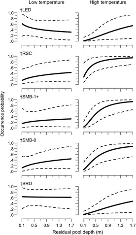
Species occurrence probability (hereafter occurrence) varied in relation to both site‐ and reach‐scale covariates, with differences between ecoregions. The final model retained site‐scale percent pool, percent vegetation, and RPD and reach‐scale water temperature, drainage area, and percent agriculture (see Appendix A for criteria). All species had a water temperature relationship, with some variation in occurrence between ecoregions. In the Arbuckle Uplift, occurrence decreased with increasing water temperature for least darter and southern redbelly dace but increased for redspot chub and both smallmouth bass life stages (Table A1, Figure 3). Least darter had little relationship with water temperature in the Ozark Highlands. The strength of the relationship was stronger in the Ozark Highlands for southern redbelly dace and age‐0 smallmouth bass. Redspot chub had no relationship with water temperature in the Ozark Highlands. Both redspot chub and southern redbelly dace had no occurrence relationship with the drainage area in the Ozark Highlands but had a strong positive relationship in the Arbuckle Uplift (Table A1, Figure 4). Occurrence increased with increasing drainage area in both ecoregions for both smallmouth bass age classes, with a stronger positive relationship in the Ozark Highlands. All species had a similar RPD relationship in both ecoregions that was dependent on water temperature (i.e., an interaction). The relationship was weak at lower water temperatures, but occurrence increased sharply with RPD at higher water temperatures (Table A1, Figure 5). There were single‐species occurrence relationships for percent vegetation and percent agriculture that also did not vary between ecoregions. Occurrence increased with increasing vegetation for least darter, while occurrence decreased with increasing agriculture for redspot chub (Figure 6). There was also statistical evidence of a percent vegetation and percent pool interaction. However, this resulted in only small changes in occurrence, with weak percent pool relationships at both low and high levels of vegetation (Figure A2).

FIGURE 3.

Relationship between occurrence probability and water temperature among species between ecoregions. Dashed lines are 95% credible intervals. LED is least darter, RSC is redspot chub, SMB is smallmouth bass, and SRD is southern redbelly dace. † for Arbuckle Uplift denotes relationships that met our criteria (see model selection in Appendix A). † for Ozark Highland denotes relationships that varied between ecoregions.

FIGURE 4.

Relationship between occurrence probability and drainage area among species between ecoregions. Dashed lines are 95% credible intervals. LED is least darter, RSC is redspot chub, SMB is smallmouth bass, and SRD is southern redbelly dace. † for Arbuckle Uplift denotes relationships that met our criteria (see model selection in Appendix A). † for Ozark Highland denotes relationships that varied between ecoregions.

FIGURE 5.

Relationship between occurrence probability and residual pool depth (RPD) among species at low and high‐water temperature (−1 and 1 SD, respectively). Dashed lines are 95% credible intervals. LED is least darter, RSC is redspot chub, SMB is smallmouth bass, and SRD is southern redbelly dace. † denotes water temperature‐RPD interaction terms that met our criteria (see model selection in Appendix A).

FIGURE 6.

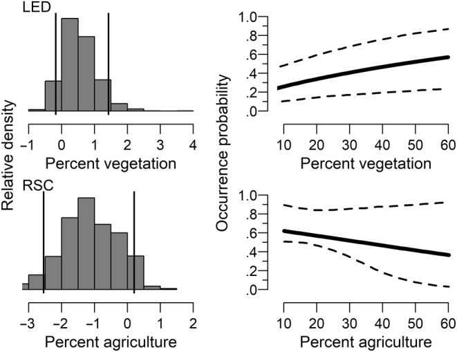
Relationship between occurrence probability and percent vegetation for least darter (LED, upper panels) and relationship between occurrence probability and percent agriculture for redspot chub (RSC, lower panels). The histograms in the left panels are a visual representation of the posterior distribution for the covariate slopes. The vertical lines approximate endpoints of 95% highest density intervals. Dashed lines in the right panels are 95% credible intervals.

4. DISCUSSION

We found that some physicochemical relationships for spring‐associated fishes differed by ecoregion, but many were similar. Although we can only speculate about the reasons, water temperature relationships differed in the two ecoregions for three of the five fishes we studied. We also found that smallmouth bass occurrence was relatively high in smaller and larger drainage areas of the Ozark Highlands, whereas bass was less likely to occur in smaller drainages of the Arbuckle Uplift. Alternatively, we found important ecological relationships were shared despite the separation in ecoregions. Most notably, we found an interaction between RPD and water temperature, regardless of ecoregion, where sites with deeper pools were more likely to be occupied by all fishes examined under higher water temperature conditions. In addition to identifying the ecological relationships of spring‐associated fishes, our findings have implications for stream‐fish conservation. In particular, instream habitat manipulations or protections may be useful strategies to counter increasing water temperatures due to climate change and other human perturbations.

Habitat degradation is a threat facing many aquatic species but has specific implications when considering future projected changes in stream water temperatures. Water temperatures in this region (MacDonald, 2010) and many others in North America (Poff et al., 2002) are rising, and projections indicate many aquatic species will make northward migrations (Ficke et al., 2007; Jackson & Mandrak, 2002; Shuter & Post, 1990). However, for narrow‐range endemic species with limits on the northward‐migration capacity (Carpenter et al., 1992), conservation efforts will likely focus on either moving populations (Galloway et al., 2016) or ensuring there is mitigation in place that will ensure persistence (Paukert et al., 2021). For example, least darter occupies catchments where downstream dispersal would be the only possible consideration without human intervention. Alternatively, managers might consider ensuring that deeper pool habitat is maintained, and groundwater connections persist (i.e., monitor groundwater withdrawals), so a natural thermal refugia is available to this and the other four species we examined. This is especially important for thermal conditions given the important role water temperature plays in the physiological and behavioral responses of fishes (Coutant, 1987) and a broader capacity as a resource fish use (Magnuson et al., 1979). Ensuring the continued persistence of key habitat patches will be important for the persistence of many riverine species.

Streams are inherently nested ecosystems; thus, it is important to understand patch dynamics and species distributions in a multiscale context (Fausch et al., 2002; Frissell et al., 1986; Gido et al., 2006). Relationships may emerge when examining environmental interactions across spatial scales. For example, water temperature was similar across adjacent sites but variable at the reach scale. We found that occurrence relationships with site‐scale pool characteristics (measured as RPD) were strongly dependent on reach‐scale water temperature for all focal species. This relationship is not surprising for larger‐bodied fishes (e.g., smallmouth bass, Dauwalter & Rahel, 2008). However, the association with deeper pools during warmer periods is interesting for smaller‐bodied species such as least darter and southern redbelly dace. The relationship between smaller‐bodied fishes and deeper pools is common in intermittent streams, where predation risk is low (Labbe & Fausch, 2000). However, understanding the dynamics between smaller and larger‐bodied species in larger streams where predation is a concern has not been well studied in warmwater streams. Coarser‐scale environmental characteristics also constrain and shape finer‐scale stream habitats (Frissell et al., 1986; Stevenson, 1997). Observed patterns in stream‐fish occurrence at a certain scale are associated with coarser‐scale factors (Mollenhauer et al., 2019). We found a higher occurrence probability with increasing drainage area for multiple species. Thus, all sites nested within a reach were more likely to be occupied in larger drainages, regardless of site‐scale characteristics.

Although fundamental to ecological research and conservation, multiscale studies are challenging and require appropriate study design and analytical approaches. Completely random or haphazard site selection does not alleviate the inevitable spatial correlation (pseudoreplication) when sampling nested systems (Fausch et al., 2002; Wagner et al., 2006). Further, sampling a single site within a coarser spatial scale (here one habitat complex per reach) does not allow for examining multiscale relationships (i.e., no replication). Rather, a multiscale design has intentional pseudoreplication (i.e., multiple habitat complexes with a reach), which can be dealt with via an applicable analysis. Multilevel (hierarchical) modeling can incorporate grouping factors to account for the lack of independence among nested observations (Gelman & Hill, 2006; Wagner et al., 2006). As we did here, covariates can also be included to identify coarser‐scale drivers of finer‐scale relationships (i.e., explain sources of spatial correlation). Multiple species can also be included in a single multilevel model but interpreted as a series of single‐species models. Due to multiple sources of error, multilevel models inherently (and appropriately) have increased uncertainty around estimates. However, a primary advantage is the ability to break a complex question into manageable pieces (i.e., isolate important relationships amidst the “noise”). Although Bayesian modeling is more “naturally” multilevel, the general approach is also readily applied in Frequentist statistics (i.e., random‐effects or mixed‐effect models; Gelman & Hill, 2006; Kéry and Royle, 2016).

Between‐ecoregion differences in habitat associations can be interesting and may play a key role in developing meaningful conservation and management strategies for fishes. For two fishes, there were relationships with water temperature in the Arbuckle Uplift but not the Ozark Highlands. For the least darter, the lack of relationship in the Ozark Highlands was likely related to the relatively few detections in that ecoregion, resulting in high uncertainty in the parameter estimate. However, the redspot chub had numerous detections and did not have a relationship between occurrence and water temperature in the Ozark Highlands (except for periods of warmer water temperatures). This may be related to biotic considerations, such as dispersal processes (Wisz et al., 2013), often not included in habitat models. Alternatively, if water temperatures do not exceed their critical maximums (i.e., 34.8°C for redspot chub, Farless & Brewer, 2017), there may be other context dependencies on this relationship. For example, sizes of redspot chub in the Ozark Highlands exhibit two feeding niche patterns (Rodger & Starks, 2021), which may relate to changing habitat patterns based on food resources available. This may be one of several reasons others show ecological relationships in some studies that are not mirrored by others. Unfortunately, studies examining one or a few rivers cannot uncover these relationships. Relationships with drainage area also differed by ecoregion for four of the five species we examined (i.e., all but least darter). Interestingly, the four species tend to be more common in the Ozark Highlands, and we see their occupancy approach a high level for all species except southern redbelly dace. One possibility is that density dependence affects how some species use their habitat. This phenomenon is documented for salmonid life stages (e.g., juvenile brown trout Lobón‐Cerviá, 2006; Lobón‐Cerviá & Mortensen, 2006). For smallmouth bass, however, the population inhabiting the Arbuckle Uplift is non‐native (Starks & Rodger, 2020), whereas a different native strain occurs in the Ozarks Highlands (Brewer & Orth, 2015).

Differences in the recent taxonomic divisions of smallmouth bass may also relate to some differences observed in occupancy relationships. Smallmouth bass in the Ozark Highlands of OK, southeast KS, and southwest MO were once considered a subspecies of smallmouth bass (Hubbs & Bailey, 1940). More recently, it has been suggested that the subspecies be elevated to the species level (Kim et al., 2022). Research in the Ozark Highlands shows the Neosho bass (M. dolomieu velox) tends to use smaller streams more so than the nominal species (Miller & Brewer, 2020; Taylor et al., 2018), which was introduced to the Arbuckle Uplift. Additionally, small streams adjacent to larger rivers are important rearing areas for the Neosho bass (Miller & Brewer, 2020). Differences in their ecology may be related to underlying differences in evolution in the Ozark Highlands. This is important as closely related species are often assumed to have similar ecological needs, which is not the case for many species and hinders our ability to designate surrogate species.

Although we outline some interesting between and within ecoregion relationships, examination of network position of physicochemical parameters would be an area where future research might focus. Smaller streams, for example, can be important rearing habitats even for top‐level predators (Meyer et al., 2007; Rosenfeld et al., 2002), and spatial proximity can be a driving factor (Smith & Kraft, 2005). For example, Miller and Brewer (2020) found that smaller streams of the Ozark Highlands adjacent to larger streams support relatively large populations of young‐of‐year Neosho bass. The adjacent larger streams provide heterogeneous habitats, including thermal patchiness (Arrigoni et al., 2008; Westhoff & Paukert, 2014), diverse foraging opportunities (Sabo et al., 1996), and refuge from disturbance, predation, and density‐dependent effects (Letcher et al., 2015; Lukas & Orth, 1995). Consequently, including network position in future studies would provide insight into the importance of habitat patches across space. Conservation efforts focused on certain portions of the landscape (i.e., springs) that are particularly ecologically meaningful may also help focus our use of limited conservation dollars.

Snorkeling in relatively clear warmwater streams is often overlooked as a sampling strategy; however, it has several advantages over more traditional sampling gears, depending on the study goal. We show an increase in detection probability while snorkeling as water depth, water clarity, and water temperature increase. Surprisingly, even at lower visibilities (~1 m), snorkeling had higher detection than seining for our target species. Others have also found that snorkeling performs as well as the comparative method (Albanese et al., 2011; Brewer & Ellersieck, 2011; Moore et al., 2017). Snorkeling offers many advantages over seining for stream fishes, such as no handling stress and less physical habitat disturbance. These advantages are especially true when studying threatened or endangered species. Snorkeling also limits harm to non‐target species and taxa. Snorkeling has also been used for reliable abundance and size‐structure estimates compared to other methods (Mullner et al., 1998; Wildman & Neumann, 2003). As with any sampling method, snorkeling may not be appropriate for all fishes. For example, detection is very low for species with cryptic coloration (Macnaughton et al., 2015) and a high affinity for cover (Mollenhauer & Brewer, 2018). Nevertheless, future sampling efforts in relatively clear warmwater streams would benefit from the consideration of snorkeling as a primary sampling method for many species after an initial evaluation. Snorkeling is a method that would add to the repertoire of standard sampling methods for warmwater North American fishes.

Habitat alterations due to landscape changes not captured by agricultural disturbance may affect species in both ecoregions (Christenson et al., 2011; Seilheimer & Fisher, 2010). We found a negative relationship between redspot chub occurrence probability and the amount of upstream agriculture, regardless of ecoregion (Figure 6). The apparent decrease in suitable habitats for spring‐associated species at several of the known historical locations could be due to a myriad of factors, including altered flow regimes (Lynch et al., 2018; Poff et al., 1997), climate change (Hu et al., 2005), or introduced species (Rahel et al., 2008). Least darter and southern redbelly dace were more widespread in the Ozark Highlands in historical collections before 1970. The Ozark Highland sites had higher percentages of agriculture, and human landscape activities can intensify patchy distributions at range edges (Sagarin et al., 2006). Our agriculture coefficient did not include other catchment‐level disturbances and may co‐vary (i.e., land use totals to 100%). Future research would benefit from directly examining the mechanisms associated with landscape perturbations (e.g., sedimentation) to determine the specific stressor.

Multiscale studies of lotic warmwater species are important for developing meaningful conservation plans (Labbe & Fausch, 2000; Torgersen et al., 2006; Wang et al., 2001). As climate change continues to alter the landscape, conservation strategies will be especially important for those species with lower thermal tolerances associated with springs or other groundwater features. Spring‐associated species rely on hyporheic flows because the constant water temperature minimizes extreme fluctuations, creates thermal refugia, and helps maintain baseflows (Bergey et al., 2008; Matthews et al., 1985; Peterson & Rabeni, 1996; Schaefer et al., 2003; Torgersen et al., 1999). Interestingly, we show how all our warmer target species occupied deeper pools during periods of warmer‐water conditions, indicating that consideration for maintaining appropriate channel morphology may benefit a variety of warmwater fishes. This may be especially important given the sheer number of warmwater fishes that have been petitioned for listing within the United States, especially the more diverse areas of the southeast (https://ecos.fws.gov/ecp/report/table/petitions‐received.html, Accessed September 15, 2023).

Managers are increasingly concerned about the persistence of warmwater fishes; our results indicate some possibilities for stream temperature mitigation, and we identify stressors that are shared across both ecoregions. Efforts to identify the mechanistic underpinning of these ecological relationships would be helpful to discern if some of the different ecoregion relationships represent warning signals caused by physicochemical stressors. For example, do the shifting temperature relationships in the two ecoregions signal concerns related to survival and growth, or is this a plastic response to shifting prey resources (and therefore a tradeoff with water temperature conditions)? Our results also indicate that channel mitigation to maintain reaches with deeper pool habitats may be an important strategy for maintaining thermal refugia during warmer water temperatures. For example, preventing gravel removal is a management strategy aimed at preventing the widening and shallowing of stream channels. Moreover, some agricultural and urban land uses cause the widening and shallowing of stream channels (Kayitesi et al., 2022; Konrad & Booth, 2005), particularly when the riparian corridor has not been properly maintained (Lovell & Sullivan, 2006; Naiman & Decamps, 1997). Although we recognize that species are plastic and that may relate to resilience to climate change (Seebacher et al., 2015), it is unclear whether thermally sensitive warmwater fishes can adapt their thermal tolerances at a rate that keeps up with warming trends. It will become increasingly important to identify strategies that will provide apparent refugia if the goal is to conserve many of our warmwater fishes.

AUTHOR CONTRIBUTIONS

Dusty Swedberg: Conceptualization (equal); data curation (lead); formal analysis (equal); funding acquisition (supporting); investigation (equal); methodology (lead); project administration (supporting); writing – original draft (lead); writing – review and editing (supporting). Robert Mollenhauer: Conceptualization (supporting); data curation (supporting); formal analysis (equal); funding acquisition (supporting); investigation (equal); methodology (equal); project administration (supporting); visualization (supporting); writing – review and editing (equal). Shannon K. Brewer: Conceptualization (lead); data curation (supporting); formal analysis (supporting); funding acquisition (lead); investigation (equal); methodology (equal); project administration (lead); supervision (lead); writing – original draft (equal); writing – review and editing (lead).

APPENDIX A.

A.1. Covariate transformations and pairwise correlations

Prior to fitting models, we made data transformations to improve linearity and checked multicollinearity among covariates. We natural‐log transformed water velocity, discharge, drainage area, residual pool depth, and site area due to right‐skewed distributions. We improved symmetry for percent vegetation, percent coarse wood, and percent fine substrate using a square‐root transformation. We used Pearson's pairwise correlation coefficient (r) to examine multicollinearity. There were no strong correlations between our detection covariates (|r| ≤ .26). We removed discharge and total area from our occurrence covariate set because they were strongly positively correlated with drainage area (|r| ≥ .89). The final occurrence covariate set maintained |r| ≤ .54.

A.2. Model equations

We write the detection equation as:

$$\begin{array}{cc}\text{logit}\left(p_{\mathit{ijk}}\right)\hfill & ={\mathrm{\alpha }}_i+{\mathrm{\alpha }}_{\text{1i}}{E}_j+{\mathrm{\alpha }}_{2i}{G}_{\mathit{jk}}+{\sum }_{n=1}^7{\beta }_n{X}_{\mathit{njk}}\hfill \\ \hfill & +{\mathrm{\beta }}_8{X}_{7\mathit{jk}}^2+{{\sum }_{b=9}^{15}\sum }_{n=1}^7{\beta }_b{X}_{\mathit{njk}}{G}_{\mathit{jk}}+{\mathrm{\beta }}_{16}{X}_{7\mathit{jk}}^2{G}_{\mathit{jk}.}\hfill \end{array}$$

for i = 5, for j = 153, for k = 1, 2, … K

$$\mathrm{\alpha }~\mathit{\text{Gaussian}}\left({\mathrm{\mu }}_{\mathrm{\alpha }},{\sigma }_{\alpha }^2\right),{\mathrm{\alpha }}_1~\mathit{\text{Gaussian}}\left({\mathrm{\mu }}_{\text{α1}},{\sigma }_{\alpha 1}^2\right),{\mathrm{\alpha }}_2~\mathit{\text{Gaussian}}\left({\mathrm{\mu }}_{\text{α2}},{\sigma }_{\alpha 2}^2\right),$$

where α is the species intercept, α₁ is the ecoregion E coefficient, α₂ is the gear G coefficient, β₁–β₇ are main effect coefficients for associated covariates mean velocity X ₁, percent coarse wood X ₂, percent coarse substrate X ₃, clarity X ₄, temperature X ₅, percent vegetation X ₆, and water depth X ₇ (main effect is the coefficient for the first‐order quadratic term), β₈ is the coefficient second‐order quadratic water depth term, β₉–β₁₅ are gear interaction coefficients for associated covariates X ₁–X _7, β₁₆ is the gear interaction coefficient for the second‐order quadratic water depth term, υ is a normality parameter, μ is the group mean hyperparameter, and σ² is variance. We used a t‐distribution, rather than a normal distribution, for the reach grouping factor to account for heavy tails and improve model fit (Kruschke 2013; Lee and Thompson 2008).

We write the occurrence equation as:

$$\begin{array}{cc}\text{logit}\left({\mathrm{\Psi }}_{\mathit{ijm}}\right)\hfill & ={\mathrm{\alpha }}_i+{\mathrm{\alpha }}_{\text{1i}}{E}_j+{\mathrm{\alpha }}_{2i}{T}_j+{\sum }_{n=1}^9{\beta }_{\mathit{ni}}{X}_{\mathit{nj}}\hfill \\ \hfill & +{\mathrm{\beta }}_{10i}{X}_{1j}{X}_{\text{8j}}+{\mathrm{\beta }}_{11i}{X}_{6j}{X}_{\text{8j}}+{\mathrm{\beta }}_{12i}{X}_{5j}{X}_{\text{6j}}+{\sum }_{n=13}^{22}{\mathrm{\beta }}_{\mathit{ni}}{E}_j{X}_{\mathit{nj}}\hfill \\ \hfill & +{\mathrm{\tau }}_{im},\text{for}i=5,\text{for}j=153,\text{for}m=61,\hfill \end{array}$$

$$\begin{array}{c}\mathrm{\alpha }~\text{Gaussian}\left({\mathrm{\mu }}_{\mathrm{\alpha }},{\sigma }_{\alpha }^2\right),{\mathrm{\alpha }}_1~\text{Gaussian}\left({\mathrm{\mu }}_{\text{α1}},{\sigma }_{\alpha 1}^2\right),\hfill \\ {\mathrm{\alpha }}_2~\text{Gaussian}\left({\mathrm{\mu }}_{\text{α2}},{\sigma }_{\alpha 2}^2\right),\hfill \\ {\mathrm{\beta }}_{1–22}~\text{Gaussian}\left({\mu }_{\beta 1–13,}{\sigma }_{\beta 1–13}^2\right),\mathrm{\tau }~t\left(0,{{\sigma }_{\tau }^2}_{,}{\mathrm{\upsilon }}_{\mathrm{\tau }}\right),\hfill \end{array}$$

where α is the species intercept, α₁ is the ecoregion E coefficient, α₂ is the year T coefficient, β₁–β₉ are main effects coefficients or slopes for associated covariates mean temperature X ₁, percent coarse wood X ₂, percent fine substrate X ₃, percent agriculture X ₄, percent pool X ₅, percent vegetation X ₆, groundwater contribution X ₇, RPD X ₈, and drainage area X ₉, β₁₀ is the mean temperature * RPD interaction coefficient, β₁₁ is the percent vegetation * RPD interaction coefficient, β₁₂ is the proportion pool * percent vegetation interaction coefficient, β₁–β₉ are coefficients for the ecoregion * covariate interaction terms, τ is the reach grouping factor, μ is the group mean hyperparameter, and σ is variance.

A.3. Model selection

We simplified the occupancy model by removing covariates with a backward‐selection process. We began by removing gear‐detection covariate interaction terms if the absolute value of the mode (most likely value) in the posterior distribution was less than both endpoints of the 95% highest density interval (HDI) for the coefficient. This approach alleviated coefficients being removed for HDIs that slightly overlapped zero using a Frequentist‐like cutoff rule and shifted the focus from significance to effect size and uncertainty. Unlike confidence intervals that only provide endpoints, posterior distributions, and associated HDIs are direct expressions of effect size and uncertainty that can be expressed visually as a probability distribution (Kruschke and Liddell 2018). For retained terms, there was support for either a positive or negative relationship with the uncertainty primarily on the true effect size (see Figure 6 in the Results for an example). We refitted the model and used the same criteria to remove or retain the main effects without a gear interaction. A covariate interaction or main effect was retained if there was support of a relationship for at least one species. We considered retained ecoregion and gear interactions variable (e.g., the relationship between clarity and detection varied by gear type) and covariate interactions a dependency of one covariate relationship on levels of the other (e.g., the relationship between occurrence and residual pool depth was dependent on water temperature). We used the same process and criteria to simplify the occurrence component of the model, starting with ecoregion‐covariate interactions. We present occurrence and detection relationships visually in the Results, with the full output provided in the Appendix A (Table A1).

A.4. JAGS specifications and diagnostics

Posterior distributions for coefficients were estimated with Markov chain Monte Carlo (MCMC) methods. We used truncated vague normal priors (Kéry and Shaub 2012; Kéry and Royle 2016) for group‐mean hyperparameters, vague gamma priors for associated standard deviations (Plummer 2003), and a shifted exponential prior for the occurrence reach grouping factor normality parameter (Kruschke 2013). Adequate MCMC convergence (chain mixing) was achieved using four chains of 50,000 iterations each ran in parallel after a 25,000‐iteration burn‐in phase (thinning = 100). We considered convergence a potential scale reduction factor < 1.05 (Brooks and Gelman 1998). We calculated HDIs using the R package HDInterval (Meredith and Kruschke 2022).

We examined model fit using a posterior predictive check (Conn et al. 2018; Kéry and Royle 2016). We simulated expected y _js under model parameters to compare discrepancies with observed y _js and calculated a Bayesian p‐value. A Bayesian p‐value near 0.5 suggests adequate fit and extreme values (i.e., <0.05 or >0.95) indicate a lack of fit. We also examined a plot of the discrepancy (i.e., residual error) of simulated data versus the discrepancy of observed data. A random scattering of values around the diagonal equality line supports a good fit. The Bayesian p‐value was 0.57 and the visual assessment confirmed adequate fit.

TABLE A1.

Multispecies occupancy model output on the logit scale as the mode (most likely value) with a 95% highest density interval (HDI).

Coefficient	Mode (90% HDI)
Occurrence probability
LED – Arbuckle Uplift, 2018	−0.11 (−1.73, 1.56)
LED – Ozark Highlands	−6.32 (−13.30, 2.46)
LED – 2019	−1.60 (−3.29, 0.12)
LED – water temperature (Arbuckle Uplift) a	−0.81 (−2.00, 0.25)
LED – water temperature (Ozark Highlands)	−0.45 (−4.34, 3.59)
LED – drainage area (Arbuckle Uplift)	0.26 (−0.85, 1.29)
LED – drainage area (Ozark Highlands)	2.20 (−2.47, 5.30)
LED – percent agriculture	0.05 (−1.32, 1.40)
LED – percent pool	−0.14 (−1.03, 0.57)
LED – RPD	0.56 (−0.76, 1.41)
LED – percent vegetation a	0.48 (−0.45, 1.47)
LED – RPD * water temperature a	0.94 (0.12, 2.29)
LED – percent pool * percent vegetation a	0.38 (−0.31, 1.18)
LED – reach SD	1.24 (0.01, 3.50)
RSC – Arbuckle Uplift, 2018	0.71 (−0.69, 2.74)
RSC – Ozark Highlands	4.53 (1.02, 8.72)
RSC – 2019	−1.55 (−2.96, −0.08)
RSC – water temperature (Arbuckle Uplift) a	1.06 (0.07, 2.08)
RSC – water temperature (Ozark Highlands) a	−1.75 (−5.50, 1.13)
RSC – drainage area (Arbuckle Uplift)	0.39 (−0.49, 1.39)
RSC – drainage area (Ozark Highlands) a	3.31 (0.19, 6.44)
RSC – percent agriculture a	−1.16 (−2.69, 0.41)
RSC – percent pool	−0.04 (−0.67, 0.73)
RSC – RPD a	0.81 (0.18, 1.64)
RSC – percent vegetation	−0.11 (−0.73, 0.54)
RSC – RPD * water temperature a	0.34 (−0.25, 1.04)
RSC – percent pool * percent vegetation	−0.01 (−0.75, 0.54)
RSC – reach SD	2.11 (0.66, 0.44)
SMB‐1+ − Arbuckle Uplift, 2018	0.18 (−1.37, 2.08)
SMB‐1+ − Ozark Highlands	1.59 (−1.36, 4.12)
SMB‐1+ − 2019	−1.50 (−3.03, 0.05)
SMB‐1+ − water temperature (Arbuckle Uplift) a	0.69 (−0.67, 2.08)
SMB‐1+ − water temperature (Ozark Highlands)	−0.34 (−3.25, 3.14)
SMB‐1+ − drainage area (Arbuckle Uplift) a	2.55 (0.27, 6.27)
SMB‐1+ − drainage area (Ozark Highlands) a	2.98 (0.12, 5.68)
SMB‐1+ − percent agriculture	−0.31 (−1.68, 1.02)
SMB‐1+ − percent pool	0.29 (−0.49, 1.58)
SMB‐1+ − RPD a	1.06 (0.13, 2.38)
SMB‐1+ − percent vegetation	−0.01 (−0.94, 0.81)
SMB‐1+ − RPD * water temperature a	0.79 (−0.05, 1.97)
SMB‐1+ − percent pool * percent vegetation	0.21 (−0.58, 1.04)
SMB‐1+ − reach SD	2.10 (0.59, 4.44)
SMB‐0 – Arbuckle Uplift, 2018	0.28 (−1.08, 1.55)
SMB‐0 – Ozark Highlands	2.73 (0.03, 5.63)
SMB‐0 – 2019	−1.70 (−3.43, −0.16)
SMB‐0 – water temperature (Arbuckle Uplift) a	0.59 (−0.47, 1.60)
SMB‐0 – water temperature (Ozark Highlands) a	2.30 (−1.55, 7.20)
SMB‐0 – drainage area (Arbuckle Uplift) a	0.82 (−0.17, 1.90)
SMB‐0 – drainage area (Ozark Highlands) a	3.40 (0.38, 6.37)
SMB‐0 – percent agriculture	0.52 (−0.76, 2.26)
SMB‐0 – percent pool	−0.08 (−0.84, 0.78)
SMB‐0 – RPD a	1.01 (0.16, 2.10)
SMB‐0 – percent vegetation	−0.13 (−0.95, 0.62)
SMB‐0 – RPD * water temperature a	0.53 (−0.48, 1.21)
SMB‐0 – percent pool * percent vegetation a	0.44 (−0.15, 1.24)
SMB‐0 – reach SD	2.51 (0.72, 4.90)
SRD – Arbuckle Uplift, 2018	0.13 (−1.39, 1.53)
SRD – Ozark Highlands	−2.11 (−5.45, 0.63)
SRD – 2019	−1.44 (−2.92, 0.14)
SRD – water temperature (Arbuckle Uplift) a	−1.32 (−2.89, −0.08)
SRD – water temperature (Ozark Highlands) a	−6.35 (−11.80, −0.36)
SRD – drainage area (Arbuckle Uplift)	−0.03 (−1.16, 1.05)
SRD – drainage area (Ozark Highlands) a	2.93 (0.18, 5.36)
SRD – percent agriculture	0.18 (−1.09, 1.55)
SRD – percent pool	−0.24 (−1.20, 0.49)
SRD – RPD a	0.61 (−0.39, 1.49)
SRD – percent vegetation	0.07 (−0.61, 0.88)
SRD – RPD * water temperature a	0.66 (−0.09, 1.92)
SRD – percent pool * percent vegetation a	0.33 (−0.26, 0.93)
SRD – reach SD	1.84 (0.44, 3.92)
Detection probability
LED – Arbuckle Uplift, seining	−0.13 (−0.86, 0.77)
LED – Ozark Highlands	−0.73 (−4.69, 0.43)
LED – snorkeling	1.35 (0.29, 2.57)
RSC – Arbuckle Uplift, seining	−0.21 (−0.74, 0.38)
RSC – Ozark Highlands	−0.74 (−1.39, −0.04)
RSC – snorkeling	2.84 (2.23, 3.42)
SMB‐1+ − Arbuckle Uplift, seining	−3.21 (−4.48, −2.07)
SMB‐1+ − Ozark Highlands	0.09 (−0.82, 1.15)
SMB‐1+ − snorkeling	4.52 (3.58, 5.72)
SMB‐0 – Arbuckle Uplift, seining	−0.87 (−1.61, 0.03)
SMB‐0 – Ozark Highlands	−0.17 (−0.95, 0.70)
SMB‐0 – snorkeling	2.51 (1.87, 3.20)
SRD – Arbuckle Uplift, seining	−0.47 (−1.13, 0.29)
SRD – Ozark Highlands	0.40 (−0.32, 1.11)
SRD – snorkeling	1.93 (1.25, 2.71)
Velocity (seining and snorkeling) a	−0.13 (−0.28, 0.01)
Clarity (seining) a	0.34 (0.10, 0.54)
Clarity (snorkeling) a	0.27 (−0.09, 0.65)
Water temperature (seining)	−0.07 (−0.31, 0.16)
Water temperature (snorkeling) a	0.25 (−0.16, 0.60)
Depth (seining)	0.08 (−0.12, 0.30)
Depth2 (seining)	−0.03 (−0.20, 0.13)
Depth (snorkeling) a	0.47 (0.15, 0.79)
Depth2 (snorkeling) a	−0.19 (−0.38, 0.12)

Note: Coefficients for occurrence covariate relationships with the Ozark Highlands ecoregion represent the difference from the Arbuckle Uplift ecoregion. Coefficients for detection covariate relationships with snorkeling represent the difference from seining.

Abbreviations: LED, least darter; RPD, residual pool depth; RSC, redspot chub; SD, standard deviation; SMB, smallmouth bass; SRD, southern redbelly dace.

^a Variable covariate relationships (see model selection for criteria).

FIGURE A1.

Relationship between fish detection probability and physicochemical covariates by gear type that met our criteria (see model selection in Appendix A). Dashed lines are 95% credible intervals.

FIGURE A2.

Relationship between occurrence probability and percent pool among fish species at low and high percent vegetation (−1 and 1 SD, respectively). Dashed lines are 95% credible intervals. LED is least darter, RSC is redspot chub, SMBa is age‐1 + smallmouth bass, SMBs is age‐0 smallmouth bass, and SRD is southern redbelly dace. † denotes important percent vegetation‐percent pool interaction terms that met our criteria (see model selection in Appendix A).

Any use of trade, firm, or product names is for descriptive purposes only and does not imply endorsement by the U.S. Government.

Swedberg, D. A. , Mollenhauer, R. , & Brewer, S. K. (2023). The context dependency of fish‐habitat associations in separated karst ecoregions. Ecology and Evolution, 13, e10701. 10.1002/ece3.10701

DATA AVAILABILITY STATEMENT

Data from this study are available at https://datadryad.org/stash/share/WjyFq4‐gSU8c7jUgtGN741DIsvxcbi8ZOemxEwgFciQ (Dusty Swedberg, swedberg@illinois.edu).

REFERENCES

- Brooks, S. P. , & Gelman, A. (1998). General methods for monitoring convergence of iterative simulations. Journal of Computational and Graphical Statistics, 7, 434–455. [Google Scholar]
- Conn, P. B. , Johnson, D. S. , Williams, P. J. , Melin, S. R. , & Hooten, M. B. (2018). A guide to Bayesian model checking for ecologists. Ecological Monographs, 88, 526–542. [Google Scholar]
- Kéry, M. , & Schaub, M. (2012). Bayesian Population Analysis Using WinBUGS, Bayesian Population Analysis Using WinBUGS. Academic Press. [Google Scholar]
- Kruschke, J. K. (2013). Bayesian estimation supersedes the t test. Journal of Experimental Psychology: General, 142, 573–603. [DOI] [PubMed] [Google Scholar]
- Kruschke, J. K. , & Liddell, T. M. (2018). The Bayesian New Statistics: Hypothesis testing, estimation, meta‐analysis, and power analysis from a Bayesian perspective. Psychonomic Bulletin and Review, 25, 178–206. [DOI] [PubMed] [Google Scholar]
- Lee, K. J. , & Thompson, S. G. (2008). Flexible parametric models for random‐effects distributions. Statistics in Medicine, 27, 418–434. [DOI] [PubMed] [Google Scholar]
- Meredith, M. , & Kruschke, J. K. (2022). HDInterval: Highest (posterior) density intervals. https://cran.r‐project.org/web/packages/HDInterval/HDInterval.pdf
- Albanese, B. , Angermeier, P. L. , & Dorai‐Raj, S. (2004). Ecological correlates of fish movement in a network of Virginia streams. Canadian Journal of Fisheries and Aquatic Sciences, 61(6), 857–869. [Google Scholar]
- Albanese, B. , Owers, K. A. , Weiler, D. A. , & Pruitt, W. (2011). Estimating occupancy of rare fishes using visual surveys, with a comparison to backpack electrofishing. Southeastern Naturalist, 10(3), 423–442. [Google Scholar]
- Arrigoni, A. S. , Poole, G. C. , Mertes, L. A. , O'Daniel, S. J. , Woessner, W. W. , & Thomas, S. A. (2008). Buffered, lagged, or cooled? Disentangling hyporheic influences on temperature cycles in stream channels. Water Resources Research, 44(9), 1–13. [Google Scholar]
- Bearlin, A. R. , Schreiber, E. S. G. , Nicol, S. J. , Starfield, A. M. , & Todd, C. R. (2002). Identifying the weakest link: Simulating adaptive management of the reintroduction of a threatened fish. Canadian Journal of Fisheries and Aquatic Sciences, 59(11), 1709–1716. [Google Scholar]
- Berendzen, P. B. , Dugan, J. F. , & Gamble, T. (2010). Post‐glacial expansion into the Paleozoic plateau: Evidence of an Ozarkian refugium for the Ozark minnow Notropis nubilus (Teleostei: Cypriniformes). Journal of Fish Biology, 77(5), 1114–1136. [DOI] [PubMed] [Google Scholar]
- Berendzen, P. B. , Simons, A. M. , Wood, R. M. , Dowling, T. E. , & Secor, C. L. (2008). Recovering cryptic diversity and ancient drainage patterns in eastern North America: Historical biogeography of the Notropis rubellus species group (Teleostei: Cypriniformes). Molecular Phylogenetics and Evolution, 46(2), 721–737. [DOI] [PubMed] [Google Scholar]
- Bergey, E. A. , Matthews, W. J. , & Fry, J. E. (2008). Springs in time: Fish fauna and habitat changes in springs over a 20‐year interval. Aquatic Conservation: Marine and Freshwater Ecosystems, 18, 829–838. [Google Scholar]
- Biggs, J. , von Fumetti, S. , & Kelly‐Quinn, M. (2017). The importance of small waterbodies for biodiversity and ecosystem services: Implications for policy makers. Hydrobiologia, 793, 3–39. [Google Scholar]
- Brewer, S. K. (2013a). Groundwater influences on the distribution and abundance of riverine smallmouth bass, Micropterus dolomieu, in pasture landscapes of the midwestern USA. River Research and Applications, 29, 269–278. [Google Scholar]
- Brewer, S. K. (2013b). Channel unit use by smallmouth bass: Do land‐use constraints or quantity of habitat matter? North American Journal of Fisheries Management, 33(2), 351–358. [Google Scholar]
- Brewer, S. K. , & Ellersieck, M. R. (2011). Evaluating two observational sampling techniques for determining the distribution and detection probability of age‐0 smallmouth bass in clear, warmwater streams. North American Journal of Fisheries Management, 31(5), 894–904. [Google Scholar]
- Brewer, S. K. , Mollenhauer, R. , Alexander, J. , & Moore, D. (2022). Critical thermal maximum values for stream fishes, including distinct populations of smallmouth bass. North American Journal of Fisheries Management, 42(2), 352–360. [Google Scholar]
- Brewer, S. K. , & Orth, D. J. (2015). Smallmouth bass Micropterus dolomieu Lacepède, 1802. American Fisheries Society Symposium, 82, 9–26. [Google Scholar]
- Burr, B. M. , & Page, L. M. (1979). The life history of the least darter, Etheostoma microperca in the Iroquois river, Illinois. University of Illinois Natural History Survey Biological Notes. https://archive.org/details/lifehistoryoflea112burr [Google Scholar]
- Buth, D. G. , & Mayden, R. L. (1981). Taxonomic status and relationships among populations of Notropis pilsbryi and N. zonatus (Cypriniformes: Cyprinidae) as shown by the Glucosephosphate isomerase, lactate dehydrogenase and phosphoglucomutase enzyme systems. Copeia, 1981(3), 583–590. [Google Scholar]
- Caissie, D. (2006). The thermal regime of rivers: A review. Freshwater Biology, 51(8), 1389–1406. [Google Scholar]
- Carpenter, S. R. , Fisher, S. G. , Grimm, N. B. , & Kitchell, J. F. (1992). Global change and fresh‐water ecosystems. Annual Review of Ecology, Evolution, and Systematics, 23(1), 119–139. [Google Scholar]
- Christenson, S. , Osborn, N. I. , Neel, C. R. , Faith, J. R. , Blome, C. D. , Puckette, J. , & Pantea, M. P. (2011). Hydrogeology and simulation of groundwater flow in the Arbuckle‐Simpson aquifer, south‐Central Oklahoma. Survey Scientific Investigations Report, 2011–5029.
- Constantz, J. (1998). Interaction between stream temperature, streamflow, and groundwater exchanges in alpine streams. Water Resources Research, 34(7), 1609–1615. [Google Scholar]
- Cordes, L. E. , & Page, L. M. (1980). Feeding chronology and diet composition of two darters (Percidae) in the Iroquois River system, Illinois. The American Midland Naturalist, 104(1), 202–206. [Google Scholar]
- Coutant, C. C. (1987). Thermal preference: When does an asset become a liability? Environmental Biology of Fishes, 18(3), 161–172. [Google Scholar]
- Dauwalter, D. C. , & Rahel, F. J. (2008). Distribution modelling to guide stream fish conservation: An example using the mountain sucker in the Black Hills National Forest, USA. Aquatic Conservation: Marine and Freshwater Ecosystems, 18(7), 1263–1276. [Google Scholar]
- Dewald, T. (2014). NHD Plus Version 2: User Guide.
- Dodd, H. R. , Peitz, D. G. , Rowell, G. A. , Bowles, D. E. , & Morrison, L. W. (2008). Protocol for monitoring fish communities in small streams in the heartland inventory and monitoring network. U.S. National Park Service. https://irma.nps.gov/DataStore/Reference/Profile/2284726
- Dorazio, R. M. , & Royle, J. A. (2005). Estimating size and composition of biological communities by modeling the occurrence of species. Journal of the American Statistical Association, 100(470), 389–398. [Google Scholar]
- Dorazio, R. M. , Royle, J. A. , Soderstrom, B. , & Glimskar, A. (2006). Estimating species richness and accumulation by modeling species occurrence and detectability. Ecology, 87(4), 842–854. [DOI] [PubMed] [Google Scholar]
- Duncan, R. S. , Elliott, C. P. , Fluker, B. L. , & Kuhajda, B. R. (2010). Habitat use of the watercress darter (Etheostoma nuchale): An endangered fish in an urban landscape. The American Midland Naturalist, 164(1), 9–21. [Google Scholar]
- Dunham, J. B. , Rosenberger, A. E. , Thurow, R. F. , Dolloff, C. A. , & Howell, P. J. (2009). Coldwater fish in wadeable streams. In Bonar S. A., Hubert W. A., & Willis D. W. (Eds.), Standard methods for sampling north American freshwater fishes (pp. 1–20). American Fisheries Society. [Google Scholar]
- Dunham, J. B. , & Vinyard, G. L. (1997). Incorporating stream level variability into analyses of site level fish habitat relationships: Some cautionary examples. Transactions of the American Fisheries Society, 126(2), 323–329. [Google Scholar]
- Farless, N. A. , & Brewer, S. K. (2017). Thermal tolerances of fishes occupying groundwater and surface‐water dominated streams. Freshwater Science, 36, 866–876. [Google Scholar]
- Fausch, K. D. , Lyons, J. , Karr, J. R. , & Angermeier, P. L. (1990). Fish communities as indicators of environmental degradation. American Fisheries Society Symposium, 8, 123–144. [Google Scholar]
- Fausch, K. D. , Torgersen, C. E. , Baxter, C. V. , & Li, H. W. (2002). Landscapes to riverscapes: Bridging the gap between research and conservation of stream fishes. Bioscience, 52(6), 483–498. [Google Scholar]
- Ficke, A. D. , Myrick, C. A. , & Hansen, L. J. (2007). Potential impacts of global climate change on freshwater fisheries. Reviews in Fish Biology and Fisheries, 17, 581–613. [Google Scholar]
- Frissell, C. A. , Liss, W. J. , Warren, C. E. , & Hurley, M. D. (1986). A hierarchical framework stream habitat classification: Viewing streams in a watershed context. Environmental Management, 10(2), 199–214. [Google Scholar]
- Galloway, B. T. , Muhlfeld, C. C. , Guy, C. S. , Downs, C. C. , & Fredenberg, W. A. (2016). A framework for assessing the feasibility of native fish conservation translocations: Applications to threatened bull trout. North American Journal of Fisheries Management, 36(4), 754–768. [Google Scholar]
- Gardner, C. , Coghland, S. M. , Zydlewski, J. , & Saunder, R. (2013). Distribution and abundance of stream fishes in relation to barriers: Implications for monitoring stream recovery after barrier removal. River Research and Applications, 29, 65–78. [Google Scholar]
- Gelman, A. , & Hill, J. (2006). Data analysis using regression and multilevel/hierarchical models. Cambridge University Press. [Google Scholar]
- Gido, K. B. , Falke, J. A. , Oakes, R. M. , & Hase, K. J. (2006). Fish‐habitat relations across spatial scales in prairie streams. In Hughes R. M., Wang L., & Seelbach P. W. (Eds.), Landscape influences on stream habitats and biological assemblages symposium (pp. 265–285). American Fisheries Society. [Google Scholar]
- Glazier, D. S. (1991). The fauna of north American temperate cold springs: Patterns and hypotheses. Freshwater Biology, 26(3), 527–542. [Google Scholar]
- Goldstein, R. M. , & Meador, M. R. (2004). Comparisons of fish species traits from small streams to large rivers. Transactions of the American Fisheries Society, 133(4), 971–983. [Google Scholar]
- Gordon, N. D. , McMahon, T. A. , Finlayson, B. L. , Gippel, C. J. , & Nathan, R. J. (2004). Stream hydrology: An introduction for ecologists. John Wiley and Sons. [Google Scholar]
- Gore, J. A. , Layzer, J. B. , & Mead, J. (2001). Macroinvertebrate instream flow studies after 20 years: A role in stream management and restoration. Regulated Rivers: Research & Management, 17(45), 527–542. [Google Scholar]
- Groce, M. C. , Bailey, L. L. , & Fausch, K. D. (2012). Evaluating the success of Arkansas darter translocations in Colorado: An occupancy sampling approach. Transactions of the American Fisheries Society, 141, 825–840. [Google Scholar]
- Hargrave, C. W. , & Johnson, J. E. (2003). Status of Arkansas darter, Etheostoma cragini and least darter, E. Microperca, in Arkansas. The Southwestern Naturalist, 48(1), 89–92. [Google Scholar]
- Homer, C. , Dewitz, J. , Yang, L. , Jin, S. , Danielson, P. , Xian, G. , Coulston, J. , Herold, N. , Wickham, J. , & Megown, K. (2015). Completion of the 2011 National Land Cover Database for the conterminous United States – Representing a decade of land cover change information. Photogrammetric Engineering & Remote Sensing, 81(5), 345–354. [Google Scholar]
- Hu, Q. , Willson, G. D. , Chen, X. , & Akyuz, A. (2005). Effects of climate and landcover change on stream discharge in the Ozark highlands, USA. Environmental Modeling and Assessment, 10(1), 9–19. [Google Scholar]
- Hubbs, C. (1995). Perspectives: Springs and spring runs as unique aquatic systems. Copeia, 1995(4), 989–991. [Google Scholar]
- Hubbs, C. (2001). Environmental correlates to the abundance of spring‐adapted versus stream‐adapted fishes. The Texas Journal of Science, 53, 299–326. [Google Scholar]
- Hubbs, C. L. , & Bailey, R. M. (1940). A revision of the black basses (Micropterus and Huro) with descriptions of four new forms. University of Michigan. https://deepblue.lib.umich.edu/bitstream/handle/2027.42/56293/MP048.pdf?sequence=1
- Hynes, H. B. N. (1975). The stream and its valley. Vereinigung Fur Theoretische Und Angewandte Limnologie, 19, 1–15. [Google Scholar]
- Jackson, D. A. , & Mandrak, N. E. (2002). Changing fish biodiversity: Predicting the loss of cyprind biodiversity due to global climate change. In American fisheries society symposium, 89–98. American Fisheries Society.
- Johnson, J. D. , & Hatch, J. T. (1991). Life history of the least darter Etheostoma microperca at the northwestern limits of its range. The American Midland Naturalist, 125(1), 87–103. [Google Scholar]
- Kayitesi, N. M. , Guzha, A. C. , & Mariethoz, G. (2022). Impacts of land use land cover change and climate change on river hydro‐morphology‐a review of research studies in tropical regions. Journal of Hydrology, 615, 128702. [Google Scholar]
- Kellner, K. (2021). ‘jagsUI’: A wrapper around ‘rjags’ to streamline ‘JAGS’ analyses. https://rdrr.io/cran/jagsUI/
- Kéry, M. , & Royle, J. A. (2016). Applied hierarchical modeling in ecology: Analysis of distribution, abundance and species richness in R and BUGS: Volume 1: Prelude and static models. Academic Press. [Google Scholar]
- Kim, D. , Taylor, A. T. , & Near, T. J. (2022). Phylogenomics and species delimitation of the economically important black basses (Micropterus). Scientific Reports, 12(1), 9113. [DOI] [PMC free article] [PubMed] [Google Scholar]
- Kollaus, K. A. , & Bonner, T. H. (2012). Habitat associations of a semi‐arid fish community in a karst spring‐fed stream. Journal of Arid Environments, 76, 72–79. [Google Scholar]
- Konrad, C. P. , & Booth, D. B. (2005). Hydrologic changes in urban streams and their ecological significance. In American Fisheries Society Symposium Vol. 47, No. 157, p. 17.
- Labbe, T. R. , & Fausch, K. D. (2000). Dynamics of intermittent stream habitat regulate persistence of a threatened fish at multiple scales. Ecological Applications, 10(6), 1774–1791. [Google Scholar]
- Lake, P. S. (2000). Disturbance, patchiness, and diversity in streams. Journal of the North American Benthological Society, 19(4), 573–592. [Google Scholar]
- Last, P. R. , White, W. T. , Gledhill, D. C. , Hobday, A. J. , Brown, R. , Edgar, G. J. , & Pecl, G. (2011). Long‐term shifts in abundance and distribution of a temperate fish fauna: A response to climate change and fishing practices. Global Ecology and Biogeography, 20(1), 58–72. [Google Scholar]
- Letcher, B. H. , Schueller, P. , Bassar, R. D. , Nislow, K. H. , Coombs, J. A. , Sakrejda, K. , Morrissey, M. , Sigourney, D. B. , Whiteley, A. R. , O'Donnell, M. J. , & Dubreuil, T. L. (2015). Robust estimates of environmental effects on population vital rates: An integrated capture‐recapture model of seasonal brook trout growth, survival and movement in a stream network. Journal of Animal Ecology, 84(2), 337–352. [DOI] [PubMed] [Google Scholar]
- Lisle, T. E. (1987). Using “residual depths” to monitor pool depths independently of discharge. U.S. Forest Service, Research Note PSW‐394.
- Lobón‐Cerviá, J. (2006). Instability of stream salmonid population dynamics under strong environmental limitations – A reply. Oikos, 114(2), 376–380. [Google Scholar]
- Lobón‐Cerviá, J. , & Mortensen, E. (2006). Two‐phase self‐thinning in stream‐living juveniles of lake‐migratory brown trout Salmo trutta L. compatibility between linear and non‐linear patterns across populations? Oikos, 113(3), 412–423. [Google Scholar]
- Lovell, S. T. , & Sullivan, W. C. (2006). Environmental benefits of conservation buffers in the United States: Evidence, promise, and open questions. Agriculture, Ecosystems & Environment, 112(4), 249–260. [Google Scholar]
- Lukas, J. A. , & Orth, D. J. (1995). Factors affecting nesting success of smallmouth bass in a regulated Virginia stream. Transactions of the American Fisheries Society, 124(5), 726–735. [Google Scholar]
- Lynch, D. T. , Leasure, D. R. , & Magoulick, D. D. (2018). The influence of drought on flow‐ecology relationships in Ozark Highland streams. Freshwater Biology, 63(8), 946–968. [Google Scholar]
- MacDonald, G. M. (2010). Water, climate change, and sustainability in the southwest. Proceedings of the National Academy of Sciences, 107(50), 21256–21262. [DOI] [PMC free article] [PubMed] [Google Scholar]
- MacKenzie, D. I. , Nichols, J. D. , Lachman, G. B. , Droege, S. , Royle, J. A. , & Langtimm, C. A. (2002). Estimating site occupancy rates when detection probabilities are less than one. Ecology, 83(8), 2248–2255. [Google Scholar]
- Macnaughton, C. J. , Harvey‐Lavoie, S. , Senay, C. , Lanthier, G. , Bourque, G. , Legendre, P. , & Boisclair, D. (2015). A comparison of electrofishing and visual surveying methods for estimating fish community structure in temperate rivers. River Research and Applications, 31(8), 1040–1051. [Google Scholar]
- Magnuson, J. J. , Crowder, L. B. , & Medvick, P. A. (1979). Temperature as an ecological resource. American Zoologist, 19(1), 331–343. [Google Scholar]
- Magoulick, D. D. , & Kobza, R. M. (2003). The role of refugia for fishes during drought: A review and synthesis. Freshwater Biology, 48(7), 1186–1198. [Google Scholar]
- Marsh‐Matthews, E. , & Matthews, W. J. (2000). Geographic, terrestrial and aquatic factors: Which most influence the structure of stream fish assemblages in the midwestern United States? Ecology of Freshwater Fish, 9(1–2), 9–21. [Google Scholar]
- Matthews, W. J. , Hoover, J. J. , & Milstead, W. B. (1985). Fishes of Oklahoma springs. The Southwestern Naturalist, 30(1), 23–32. [Google Scholar]
- McKeown, F. A. , Jones‐Cecil, M. , Askew, B. L. , & McGrath, M. A. (1988). Analysis of stream profile data and inferred tectonic activity, eastern Ozark mountain region. U.S. Geological Survey Bulletin 1807.
- Meyer, J. L. , Strayer, D. L. , Wallace, J. B. , Eggert, S. L. , Helfman, G. S. , & Leonard, N. E. (2007). The contribution of headwater streams to biodiversity in river networks. Journal of the American Water Resources Association, 43(1), 86–103. [Google Scholar]
- Miller, A. D. , & Brewer, S. K. (2020). Age‐0 smallmouth bass abundance depends on physicochemical conditions and stream network position. Ecosphere, 11(9), e03245. [Google Scholar]
- Miller, A. D. , & Brewer, S. K. (2021). Riverscape nesting dynamics of Neosho smallmouth bass: To cluster or not to cluster? Diversity and Distributions, 27(6), 1–14. [Google Scholar]
- Mollenhauer, R. , & Brewer, S. K. (2018). Efficiency of sampling sunfishes using snorkeling in clear, warm‐water streams of the south‐Central United States. Journal of Fish and Wildlife Management, 9(2), 602–609. [Google Scholar]
- Mollenhauer, R. , Zhou, Y. , & Brewer, S. K. (2019). Multiscale habitat factors explain variability in stream fish occurrence in the Ozark highlands ecoregion, USA. Copeia, 107(2), 219–231. [Google Scholar]
- Moore, M. J. , Orth, D. J. , & Frimpong, E. A. (2017). Occupancy and detection of clinch dace using two gear types. Journal of Fish and Wildlife Management, 8(2), 530–543. [Google Scholar]
- Mullner, S. A. , Hubert, W. A. , & Wesche, T. A. (1998). Snorkeling as an alternative to depletion electrofishing for estimating abundance and length‐class frequencies of trout in small streams. North American Journal of Fisheries Management, 18(4), 947–953. [Google Scholar]
- Naiman, R. J. , & Decamps, H. (1997). The ecology of interfaces: Riparian zones. Annual Review of Ecology and Systematics, 28(1), 621–658. [Google Scholar]
- Olsen, R. L. , Chappell, R. W. , & Loftis, J. C. (2012). Water quality sample collection, data treatment and results presentation for principal components analysis – literature review and Illinois River watershed case study. Water Research, 46(9), 3110–3122. [DOI] [PubMed] [Google Scholar]
- Osborn, N. I. (2009). Arbuckle‐Simpson hydrology study. Oklahoma Water Resource Board. https://www.owrb.ok.gov/studies/groundwater/arbuckle_simpson/pdf/09_report_burec.pdf
- Park, Y. S. , Chang, J. , Lek, S. , Cao, W. , & Brosse, S. (2003). Conservation strategies for endemic fish species threatened by the three gorges dam. Conservation Biology, 17(6), 1748–1758. [Google Scholar]
- Paukert, C. , Olden, J. D. , Lynch, A. J. , Breshears, D. D. , Christopher Chambers, R. , Chu, C. , Daly, M. , Dibble, K. L. , Falke, J. , Issak, D. , & Jacobson, P. (2021). Climate change effects on north American fish and fisheries to inform adaptation strategies. Fisheries, 46(9), 449–464. [Google Scholar]
- Peck, L. S. , Souster, T. , & Clark, M. S. (2013). Juveniles are more resistant to warming than adults in 4 species of Antarctic marine invertebrates. PLoS ONE, 8(6), 1–8. [DOI] [PMC free article] [PubMed] [Google Scholar]
- Peterson, J. T. , & Rabeni, C. F. (1996). Natural thermal refugia for temperate warmwater stream fishes. North American Journal of Fisheries Management, 16(4), 738–746. [Google Scholar]
- Pflieger, W. L. (1997). The fishes of Missouri. Missouri Department of Conservation.
- Plummer, M. (2003). JAGS: A program for analysis of Bayesian graphical models using Gibbs sampling. Proceedings of the 3rd international conference on distributed statistical computing, 1–10.
- Poff, N. L. , Allan, J. D. , Bain, M. B. , Karr, J. R. , Prestegaard, K. L. , Richter, B. D. , Sparks, R. E. , & Stromberg, J. C. (1997). The natural flow regime. Bioscience, 47(11), 769–784. [Google Scholar]
- Poff, N. L. , Brinson, M. M. , & Day, J. W. (2002). Aquatic ecosystems and global climate change. Pew Center on Global Climate Change, 44, 1–36. [Google Scholar]
- Potoka, K. M. , Shea, C. P. , & Bettoli, P. W. (2016). Multispecies occupancy modeling as a tool for evaluating the status and distribution of darters in the Elk River, Tennessee. Transactions of the American Fisheries Society, 145(5), 1110–1121. [Google Scholar]
- Power, G. , Brown, R. S. , & Imhof, J. G. (1999). Groundwater and fish ‐ insights from northern North America. Hydrological Processes, 13(3), 401–422. [Google Scholar]
- R Core Team . (2019). R: A language and environment for statistical computing. R Foundation for Statistical Computing. https://www.r‐project.org/ [Google Scholar]
- Rabeni, C. F. , & Jacobson, R. B. (1993). The importance of fluvial hydraulics to fish‐habitat restoration in low‐level alluvial streams. Freshwater Biology, 29, 211–220. [Google Scholar]
- Rabeni, C. F. , Lyons, J. , Mercado‐Silva, N. , & Peterson, J. T. (2009). Warmwater fish in wadeable streams. In Bonar S. A., Hubert W. A., & Willis D. W. (Eds.), Standard methods for sampling north American freshwater fishes (pp. 43–58). American Fisheries Society. [Google Scholar]
- Rabeni, C. F. , & Sowa, S. P. (1996). Integrating biological realism into habitat restoration and conservation strategies for small streams. Canadian Journal of Fisheries and Aquatic Sciences, 53(S1), 252–259. [Google Scholar]
- Rahel, F. J. , Bierwagen, B. , & Taniguchi, Y. (2008). Managing aquatic species of conservation concern in the face of climate change and invasive species. Conservation Biology, 22(3), 551–561. [DOI] [PubMed] [Google Scholar]
- Riggs, H. C. (1972). Low‐flow investigations . Techniques of water‐resources investigations of the U.S. Geological Survey, 4th edition. United States Government Printing Office.
- Rodger, A. W. , & Starks, T. A. (2021). Ontogenetic diet shift, feeding ecology, and trophic niches of the redspot chub (Cypriniformes: Cyprinidae: Nocomis asper). Ichthyology & Herpetology, 109(3), 796–805. [Google Scholar]
- Rosenfeld, J. S. , Macdonald, S. , Foster, D. , Amrhein, S. , Bales, B. , Williams, T. , Race, F. , & Livingstone, T. (2002). Importance of small streams as rearing habitat for coastal cutthroat trout. North American Journal of Fisheries Management, 22(1), 177–187. [Google Scholar]
- Rozas, L. P. , & Odum, W. E. (1988). Occupation of submerged aquatic vegetation by fishes: Testing the roles of food and refuge. Oecologia, 77(1), 101–106. [DOI] [PubMed] [Google Scholar]
- Sabo, M. J. , Orth, D. J. , & Pert, E. J. (1996). Effect of stream microhabitat characteristics on rate of net energy gain by juvenile smallmouth bass, Micropterus Dolomieu. Environmental Biology of Fishes, 46(4), 393–403. [Google Scholar]
- Sagarin, R. D. , Gaines, S. D. , & Gaylord, B. (2006). Moving beyond assumptions to understand abundance distributions across the ranges of species. Trends in Ecology & Evolution, 21(9), 524–530. [DOI] [PubMed] [Google Scholar]
- Savino, J. F. , & Stein, R. A. (1982). Predator‐prey interaction between largemouth bass and bluegills as influenced by simulated, submersed vegetation. Transactions of the American Fisheries Society, 111(3), 255–266. [Google Scholar]
- Schaefer, J. F. , Marsh‐Matthews, E. , Spooner, D. E. , Gido, K. B. , & Matthews, W. J. (2003). Effects of barriers and thermal refugia on local movement of the threatened leopard darter, Percina Pantherina. Environmental Biology of Fishes, 66(4), 391–400. [Google Scholar]
- Schlosser, I. J. (1995). Critical landscape attributes that influence fish population dynamics in headwater streams. Hydrobiologia, 303(1–3), 71–81. [Google Scholar]
- Seebacher, F. , White, C. R. , & Franklin, C. E. (2015). Physiological plasticity increases resilience of ectothermic animals to climate change. Nature Climate Change, 5(1), 61–66. [Google Scholar]
- Seilheimer, T. S. , & Fisher, W. L. (2010). Habitat use by fishes in groundwater‐dependent streams of southern Oklahoma. The American Midland Naturalist, 164(2), 201–216. [Google Scholar]
- Shuter, B. J. , & Post, J. R. (1990). Climate, population viability, and the zoogeography of temperate fishes. Transactions of the American Fisheries Society, 119(2), 314–336. [Google Scholar]
- Smith, T. A. , & Kraft, C. E. (2005). Stream fish assemblages in relation to landscape position and local habitat variables. Transactions of the American Fisheries Society, 134(2), 430–440. [Google Scholar]
- Southwood, T. R. E. (1977). Habitat, the templet for ecological strategies? Journal of Animal Ecology, 46(2), 336–365. [Google Scholar]
- Spitale, D. (2012). A comparative study of common and rare species in spring habitats. Écoscience, 19, 80–88. [Google Scholar]
- Spyker, K. A. , & Van Den Berghe, E. P. (1995). Diurnal abundance patterns of Mediterranean fishes assessed on fixed transects by scuba‐divers. Transactions of the American Fisheries Society, 124(2), 216–224. [Google Scholar]
- Starks, T. A. , & Rodger, A. W. (2020). Otolith and scale‐based growth standards for lotic smallmouth bass. North American Journal of Fisheries Management, 40(4), 986–994. [Google Scholar]
- Stevenson, R. J. (1997). Scale‐dependent determinants and consequences of benthic algal heterogeneity. Journal of the North American Benthological Society, 16(1), 248–262. [Google Scholar]
- Taylor, A. T. , Long, J. M. , Schwemm, M. R. , & Brewer, S. K. (2018). Hybridization and genetic structure of Neosho smallmouth bass in the Ozark highlands. North American Journal of Fisheries Management, 38(6), 1226–1240. [Google Scholar]
- Thurow, R. F. (1994). Underwater methods for study of salmonids in the intermountain west. General technical report – US Department of Agriculture, Forest Service, INT‐GTR‐307.
- Torgersen, C. E. , Baxter, C. V. , Li, H. W. , & McIntosh, B. A. (2006). Landscape influences on longitudinal patterns of river fishes: Spatially continuous analysis of fish‐habitat relationships. American Fisheries Society Symposium, 2006(48), 473–492. [Google Scholar]
- Torgersen, C. E. , Price, D. M. , Li, H. W. , & McIntosh, B. A. (1999). Multiscale thermal refugia and stream habitat associations of Chinook salmon in northeastern Oregon. Ecological Applications, 9(1), 301–319. [Google Scholar]
- Tyre, A. J. , Tenhumberg, B. , Field, S. A. , Niejalke, D. , Parris, K. , & Possingham, H. P. (2003). Improving precision and reducing bias in biological surveys: Estimating false‐negative error rates. Ecological Applications, 13(6), 1790–1801. [Google Scholar]
- United States Environmental Protection Agency . (2017). Level III and IV ecoregions of the continental United States. https://19january2017snapshot.epa.gov/eco‐research/level‐iii‐and‐iv‐ecoregions‐continental‐united‐states_.html
- Vannote, R. L. , Minshall, G. W. , Cummins, K. W. , Sedell, J. R. , & Cushing, C. C. (1980). The river continuum concept. Canadian Journal of Fisheries and Aquatic Sciences, 37, 130–137. [Google Scholar]
- Vineyard, J. D. , & Feder, G. L. (1982). Springs of Missouri. Missouri Geological Survey and Water Resources, U.S. Geological Survey, and Missouri Department of Conservation. Water Resources Report no. 29.
- Wagner, T. , Hayes, C. B. , & Bremigan, M. T. (2006). Accounting for multilevel data structures in fisheries data using mixed models. Fisheries, 31(4), 180–187. [Google Scholar]
- Wall, S. S. , Berry, C. R. , Blausey, C. M. , Jenks, J. A. , & Kopplin, C. J. (2004). Fish‐habitat modeling for gap analysis to conserve the endangered Topeka shiner (Notropis topeka). Canadian Journal of Fisheries and Aquatic Sciences, 61(6), 954–973. [Google Scholar]
- Wang, L. , Lyons, J. , Kanehi, P. , & Bannerman, R. (2001). Impacts of urbanization on stream habitat and fish across multiple spatial scales. Environmental Management, 28(2), 255–266. [DOI] [PubMed] [Google Scholar]
- Wehrly, K. E. , Wiley, M. J. , & Seelbach, P. W. (2006). Influence of landscape features on summer water temperatures in lower Michigan streams. In Hughes R. M., Wang L., & Seelbach P. W. (Eds.), Landscape influences on stream habitats and biological assemblages (pp. 113–128). American Fisheries Society. [Google Scholar]
- Wentworth, C. K. (1922). A scale of grade and class terms for clastic sediments. The Journal of Geology, 30(5), 377–392. [Google Scholar]
- Westhoff, J. T. , & Paukert, C. P. (2014). Climate change simulations predict altered biotic response in a thermally heterogeneous stream system. PLoS ONE, 9(10), 1–15. [DOI] [PMC free article] [PubMed] [Google Scholar]
- Wildman, T. L. , & Neumann, R. M. (2003). Comparison of snorkeling and electrofishing for estimating abundance and size structure of brook trout and brown trout in two southern New England streams. Fisheries Research, 60, 131–139. [Google Scholar]
- Wilson, K. A. , Westphal, M. I. , Possingham, H. P. , & Elith, J. (2005). Sensitivity of conservation planning to different approaches to using predicted species distribution data. Biological Conservation, 122, 99–112. [Google Scholar]
- Wisz, M. S. , Pottier, J. , Kissling, W. D. , Pellissier, L. , Lenoir, J. , Damgaard, C. F. , Dormann, C. F. , Forchhammer, M. C. , Grytnes, J. A. , Guisan, A. , Heikkinen, R. K. , Høye, T. T. , Kühn, I. , Luoto, M. , Maiorano, L. , Nilsson, M. C. , Normand, S. , Öckinger, E. , Schmidt, N. M. , … Svenning, J. C. (2013). The role of biotic interactions in shaping distributions and realised assemblages of species: Implications for species distribution modelling. Biological Reviews, 88(1), 15–30. [DOI] [PMC free article] [PubMed] [Google Scholar]
- Wolf, S. L. , Mollenhauer, R. , & Brewer, S. K. (2019). Coldwater periods in warmwater streams: Microhabitat shifts from autumn to winter by smallmouth bass. North American Journal of Fisheries Management, 39, 1360–1372. [Google Scholar]
- Woods, A. J. , Omernik, J. M. , Butler, D. R. , Ford, J. G. , Henley, J. E. , Hoagland, B. W. , Arndt, D. S. , & Moran, B. C. (2005). Ecoregions of Oklahoma (color poster with map, descriptive text, summary tables, and photographs), U.S. Geological Survey. http://www.ecologicalregions.info/htm/ok_eco.htm
- Zhou, Y. , Fox, G. A. , Miller, R. B. , Mollenhauer, R. , & Brewer, S. K. (2018). Groundwater flux estimation in streams: A thermal equilibrium approach. Journal of Hydrology, 561, 822–832. [Google Scholar]
Associated Data
This section collects any data citations, data availability statements, or supplementary materials included in this article.