Abstract
Morbidities generally show patterns of concentration that vary by space and time. Disease mapping models are useful in estimating the spatiotemporal patterns of disease risks and are therefore pivotal for effective disease surveillance, resource allocation, and the development of prevention strategies. This study considers six spatiotemporal Bayesian hierarchical models based on two spatial conditional autoregressive priors. It could serve as a guideline on the development and application of Bayesian hierarchical models to assess the emerging risk trends, risk clustering, and spatial inequality trends, with estimation of covariables’ effects on the interested disease risk. The method is applied to the Florida Birth Record data between 2006 and 2015 to study two cardiovascular risk factors: preeclampsia and gestational diabetes. High-risk clusters were detected in North Central Florida for preeclampsia and in Central Florida for gestational diabetes. While the adjusted disease trend was stable, spatial inequality peaked in 2011–2012 for both diseases. Exposure to PM2.5 at first or/and second trimester increased the risk of preeclampsia and gestational diabetes, but the magnitude is less severe compared to previous studies. In conclusion, this study underscores the significance of selecting appropriate disease mapping models in estimating the intricate spatiotemporal patterns of disease risk and suggests the importance of localized interventions to reduce health disparities. The result also identified an opportunity to study potential risk factors of preeclampsia, as the spike of risk in North Central Florida cannot be explained by current covariables.
Keywords: Spatiotemporal modelling, Bayesian hierarchical model, Preeclampsia, Gestational diabetes, Disease mapping, Spatial inequality, Florida-USA
Introduction
The occurrence of a disease or health condition such as cancer is not randomly distributed across geographical areas; rather, it exhibits patterns of aggregation or dispersion (Cramb et al. 2017; Yin et al. 2014). Consequently, disease mapping models are proposed to smooth and visualize the spatial distribution of disease. These mapping models typically use areal data, wherein information is aggregated within defined geographic unit such as a county or census tract (Lawson 2018). These models aim to estimate the relative risk of disease in each geographic unit, especially within small administrative district or regions, by comparing the observed case count in that unit against the expected case number derived from a reference population (Waller and Carlin 2010). Therefore, they can be used to identify geographic areas with high or low disease incidence or prevalence and can help public health authorities allocate resources and develop targeted interventions (Lawson 2018).
Bayesian hierarchical models (BHM) have emerged as the preeminent choice for disease mapping since the 1990s (MacNab 2022). BHM involves the prior distribution as an underlying process model for the disease risks, which can accommodate the spatial correlation among the local disease risks either through conditional autoregressive (CAR), B-spline, or aggregation of risks on a continuous surface (Besag et al. 1991; Kottas et al. 2008; Orozco-Acosta et al. 2023; Ugarte et al. 2017). Therefore, all unknown quantities and parameters can be estimated, and the uncertainties of risk can be better quantified. In addition, the model can borrow more information from neighbors than from distant areas, smoothing the extreme values on small areas to local “neighboring” values (MacNab 2022).
Spatiotemporal extension of traditional spatial disease mapping models is an important topic, as trends can also show spatial dependence (Anderson et al. 2017). The extension can offer a more comprehensive understanding of disease dynamics, accounting for both spatial and temporal dependencies concurrently. It can be achieved through additional interaction parameters (Knorr-Held 2000), or through spatially varying but correlated risk trends, encompassing both linear and nonlinear forms (MacNab and Dean 2001; Ugarte et al. 2017). Alternative approaches amalgamate both the spatial and temporal effect in a single set of random effect (Rushworth et al. 2014).
In this study, we revisited some spatiotemporal extensions of two classical CAR priors that are widely used in the analysis of spatial count data. They were applied to model two cardiovascular disease (CVD) risk factors: preeclampsia (PE) and gestational diabetes mellitus (GDM) risk in Florida between 2006 and 2015. The objective is to assess the impact of PM2.5 more accurately while identifying the spatiotemporal pattern of PE/GDM risk in Florida. We compared six models pertinent to our data and presented the findings from the selected one.
Methodology
Relevant concepts
Standardized incidence ratio (SIR)
The use of SIR is a well-established method for disease mapping, allowing for the identification of relative risk in different geographic areas (Rioux et al. 2006). SIR is calculated by dividing the observed number of incidents by the number of cases that are “expected” in that location. In this study, we calculated expected case number for each county in Florida using data from all registered births during the study period, adjusting for mothers’ race (African American/other races), ethnicity (Hispanic/not Hispanic), age (over 35 years/35 years or under), and BMI (body mass index) (>=30 or <30).
Weight matrix
A spatial weights matrix represents the spatial structure of data. Each element defines the level of spatial connectivity between two locations (Zhou and Lin 2008). Spatial weights matrix can be roughly categorized as distance-based and contiguity-based. In this study, the spatial weight matrix W was created by first order queen contiguity, which is commonly used in disease mapping (Duncan et al. 2017). The elements of W are defined as if location is adjacent to location , and 0 otherwise. There are 67 counties in Florida, making W a 67 × 67 symmetric matrix.
Spatial autocorrelation
Spatial autocorrelation is the correlation of a variable with itself across space. The existence of spatial autocorrelation means that samples taken from nearby areas are related to each other and are not independent (Griffith 2009). Moran’s I test was used to measure the global spatial autocorrelation. Moran’s I statistics range from −1 to 1. I > 0 represents positive spatial autocorrelation (neighbors have similar values), I < 0 represents negative relationships (high values located close to low values), and I = 0 means there is no spatial autocorrelation, and the disease was randomly distributed over space (Getis 2010). In 2021, functional Moran’s I based on spatial-functional PCA was proposed to extend Moran’s I statistic to the functional context (Hassan 2021). The extended method is useful in identifying the spatial dependency over time by dimension reduction. Local Indicators of Spatial Association (LISA) was conducted through the local Moran’s I test to detect clusters of risk by measuring spatial associations in sub-regions of the study area (Getis 2010). LISA decomposes global autocorrelation into the individual observations.
Bayesian hierarchical models
We adopted Bayesian hierarchical models to incorporate complex model levels with spatial and temporal dependence structures. The general Bayesian hierarchical model for Poisson distributed spatiotemporal count data is as follows:
| (1.1) |
| (1.2) |
| (1.3) |
For areal unit k and time period , denotes the expectation of the response data . is the offsets, which are the log-transformed expected number of cases in these spatiotemporal units. is a vector of known covariates, and is a vector of regression parameters. is used to denote the latent component for areal unit and time period t, which can represent the spatiotemporal structure with one or more sets of spatiotemporally autocorrelated random effects.
There are two popular CAR priors in spatial analysis, namely BYM (Besag et al. 1991) and Leroux (Leroux et al. 2000) models. The random effects in BYM prior comprise a CAR structured spatial random effect term and an unstructured random component . The conditional distribution of can be expressed as:
| (1.4) |
and follows independent normal distribution:
| (1.5) |
In contrast to the BYM model, Leroux model has only one random effect component. The combination of spatially structured and i.i.d. variance is controlled by an additional weighting parameter , shown in Eq. (1.6):
| (1.6) |
For simplicity, defining the precision matrix as where is the vector of ones and is the identity matrix and when zero-mean is centered, the formula can be expressed as:
| (1.7) |
For the spatiotemporally autocorrelated random effects, we need to combine the spatial aspect with temporal aspect. There are various methods to achieve this goal, such as summing them together, adding interactions, or constructing a spatiotemporal random effect. In this study, we fitted four Leroux-based models using R package CARBayesST: the AR1 model, Adaptive model, ANOVA model and Separable spatial model (Lee et al. 2018). Two BYM-based models were fitted using the R-INLA package (Rue et al. 2009). A brief introduction for each model is listed in Table 1.
Table 1.
Description of models fitted in this study
| Model | Author | Description | |
|---|---|---|---|
| Leroux-based models | AR1 | Rushworth et al. (2014) | Spatially autocorrelated autoregressive of order 1 time series model. |
| Adaptive | Rushworth et al. (2017) | Extension of AR1 model. Spatially adaptive smoothing model for localized spatial smoothing. | |
| ANOVA | Knorr-Held (2000) | The spatiotemporal variation was decomposed into an overall Leroux spatial effect, an overall Leroux temporal trend, and a set of independent space-time interactions. | |
| Separable | Napier et al. (2016) | Model with an overall temporal trend and separate spatial surfaces for each time period that share a common spatial dependence parameter but have different spatial variances. | |
| BYM-based models | Linear | Bernardinelli et al. (1995) | The spatiotemporal variation was decomposed into an overall BYM spatial effect, an overall linear temporal trend, and an area-specific deviation from the trend. |
| AR1 | Knorr-Held (2000) | The spatiotemporal variation was decomposed into an overall BYM spatial effect, an overall autoregressive order 1 temporal trend, and a set of independent space-time interactions. |
Leroux-based AR1 model and Adaptive model
The AR1 model, proposed by Rushworth et al. in 2014, uses first order temporal autoregressive (AR(1)) process. Therefore, it represents the spatiotemporal structure with a multivariate AR(1) process with Leroux precision matrix.
| (2.1) |
| (2.2) |
| (2.3) |
| (2.4) |
| (2.5) |
Here, the random effects would evolve over time as a first order autoregressive process with parameter . And the spatial dependence is included through the variance of the random effects. is the conjugate prior with inverse-gamma distribution, defaulting to (1, 0.01).
The Adaptive model proposed by Rushworth et al. (2017) uses the same random effects structure as the AR1 model. But it allows for localized spatial autocorrelation by treating the non-zero elements of the weight matrix W as unknown parameters instead of one. Therefore, the study area can have different spatial dependency levels at different locations.
Leroux-based ANOVA model
The ANOVA model is modified based on Knorr-Held’s model (Knorr-Held 2000). It decomposes the spatiotemporal variation into an overall spatial effect that is common to all time periods, an overall temporal trend that is common to all spatial areas, and space-time interactions.
| (3.1) |
| (3.2) |
| (3.3) |
| (3.4) |
| (3.5) |
| (3.6) |
Here, is the spatial random effect, and is the temporal random effect. They are modelled by the Leroux priors. is the space-time interactions.
Leroux-based separable model
The separable spatial model proposed by Napier et al. in 2016 decomposes the dependence structure into an overall temporal trend but separate spatial effects. It assumes the spatial effects for each time have a common dependence parameter but different spatial variances. The model can be represented below:
| (4.1) |
| (4.2) |
| (4.3) |
| (4.4) |
| (4.5) |
Here, is the overall temporal random effect, is the separate spatial random effect at each time point, and is the temporally varying variance parameter for spatial dependence. It allows users to examine the extent to which the response’s spatial variation changed over time.
BYM-based models
The BYM-Linear model is proposed by Bernardinelli et al. (1995). It has a BYM spatial random effect, an overall linear temporal effect, and an area-specific deviation from the temporal trend. The BYM-AR1 model is a simple modification of BYM-Linear model based on Knorr-Held’s idea, changing the overall temporal effect to first order autoregressive structure, using the interactions between two unstructured random effect components.
All analysis and mapping were conducted using R (version 4.2.0). For models ran under CARBayesST package, we used 100,000 burn-ins with 50,000 samples, thinning by 10. The potential scale reduction factor proposed by Gelman et al. was used to diagnose convergence of the chains (Brooks and Gelman 1998; Gelman and Rubin 1992).
Candidate models were compared to choose the best fitting one. The model performances were evaluated by the deviance information criterion (DIC) and widely applicable information criterion (WAIC), with lower values indicating better fit. Regression estimates are presented as the means and 95% credible intervals.
Application
Study description
Gestational diabetes mellitus (GDM) is hyperglycemia first detected during pregnancy, usually develops around the 24th week of pregnancy. The incidence rate of GDM in the USA ranges from 7 to 10% in the last decade (Casagrande et al. 2018; DeSisto et al. 2014). Preeclampsia (PE), which is defined as the onset of high blood pressure during pregnancy as well as exceed protein in the urine or other end-organ damage, complicates around 3.8% of pregnancies in the USA in 2010 (Duley 2009). It usually begins after 20 weeks of pregnancy. Both PE and GDM can lead to acute and chronic adverse outcomes for the offspring and pregnant woman (Buchanan et al. 2012; Fox et al. 2019) and are associated with increased risk of future cardiovascular disease (CVD) (Sławek-Szmyt et al. 2022).
Fine particulate matter, known as PM2.5 or particulate matter with aerodynamic diameter ≤2.5 μm, is a complex mixture of solid particles and liquid droplets in the air. The components such as polycyclic aromatic hydrocarbons (PAHs) are easily absorbed through the lungs and distributed through the bloodstream (Billet et al. 2007). There is sufficient evidence associating PM2.5 with the risk of PE/GDM. A meta-analysis in 2020 indicated that a 10 μg/m3 increase of PM2.5 would enhance the risk of PE by 32% (Yu et al. 2020). Recent systematic reviews found that exposures to PM2.5 during the second trimester are significantly associated with increased risk of GDM (Hu et al. 2020; Tang et al. 2020). However, current studies considered spatial and temporal autocorrelations among PM2.5 only (Daniel et al. 2021; Zhang et al. 2019). None of these studies adjusted spatiotemporal autocorrelations among diseases.
We used the 2006 to 2015 de-identified Florida vital statistics birth data obtained from the Florida Department of Health (FDH), Bureau of Vital Statistics. More recent birth data is available but the estimated PM2.5 data we used is available only from 2000 to 2015. The birth data contained birth-related variables together with antenatal information, sociodemographic information, and any medical or labor complications experienced by the mother. The study population included all births in Florida. PE and GDM incidence data were recorded in this dataset as binary variables responding to the questions “Was mother diagnosed with gestational hypertension (pregnancy-induced hypertension, preeclampsia, etc.) during this pregnancy?” and “Was mother diagnosed with diabetes during this pregnancy?”
PM2.5 data used in this study were retrieved from the NASA Socioeconomic Data and Applications Center, with predicted PM2.5 concentrations in grid cells at a resolution of 1 km (Di et al. 2021). The prediction was generated with data from 2156 monitoring sites operated by the Environmental Protection Agency (EPA) along with other regional, or local monitoring data sets and incorporated three machine learning algorithms (Di et al. 2019). For each county-month observation, the average PM2.5 concentration was calculated using the daily data in that month of the grid points that fall within the county. The first trimester, second trimester, and 6 months cumulative exposure levels were calculated. We did not consider PM2.5 exposure after 6 months as GDM and PE would start to onset during weeks 20–24.
Because the PE risk shows seasonal variations that winter delivery has a higher risk than summer delivery, we also created a new variable to indicate the season of conception. It was dichotomized as May to July and other months according to previous studies (Rohr Thomsen et al. 2020; Verburg et al. 2018; Weinberg et al. 2017).
Descriptive results
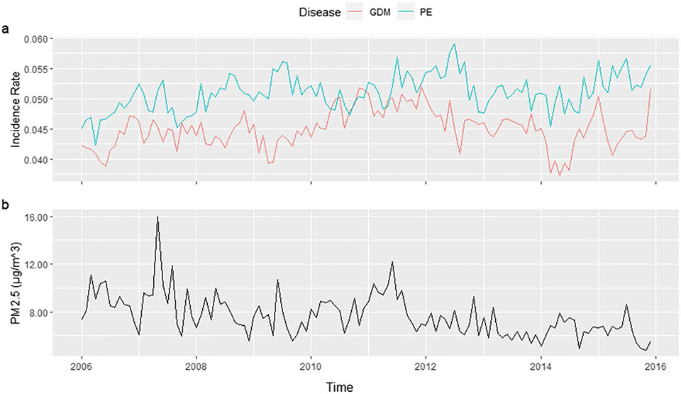
From 2006 to 2015, there were 109,817 total cases of PE and 97,086 total cases of GDM. Figure 1 shows the trend of PE, GDM, and PM2.5 in Florida between 2006 and 2015. The incidence rates of the two diseases were stable regarding the overall trend with fluctuation. The lowest PE incidence rate was 4.23% in April 2006, and the highest was 5.91% in July 2012. The GDM incidence rate ranged from 3.73 to 5.21%, in May 2014 and December 2011, respectively. On the other hand, the PM2.5 levels decreased gradually over the years. When focusing on the county level by month, number of PE cases ranges from 0 to 157, with median of 5. And GDM cases range from 0 to 132, with a median of 4. Counties with small populations such as Lafayette, Glades, and Franklin had no PE or GDM incidence for more than half of the time points, making their direct SIR ranging from 0 to 9.8. Therefore, the direct SIRs are not appropriate to be used as the risk estimation criteria.
Fig. 1.
Trend of PE, GDM, and PM2.5 in Florida, 2006–2015
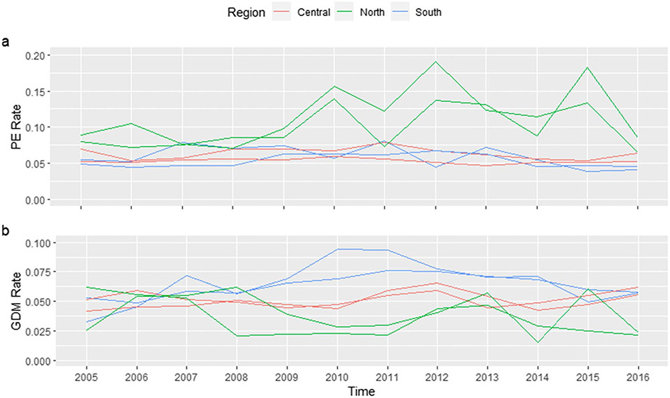
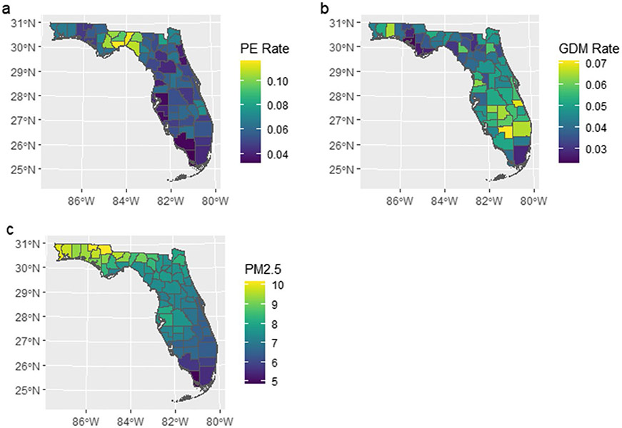
Counties in different sections of Florida showed various risk trends (Fig. 2). In addition, the risk of PE and GDM showed clear spatial inequality and positive spatial autocorrelation (Fig. 3). For counties in Central North Florida such as Wakulla and Liberty, the mean of yearly PE incidence rate was 0.112 (SD = 0.037) and 0.105 (SD = 0.052), respectively. But for counties in South Florida like Monroe and Collier, the mean of yearly PE incidence rate was only one-third of the previous rates (Monroe: 0.033, SD = 0.012; Collier: 0.035, SD = 0.005). Similar spatial inequality was observed for GDM, too.
Fig. 2.
Trend of PE and GDM risk in selected counties (North: Taylor, Wakulla; South: Hendry, Palm Beach; Central: Polk, Lake), 2006–2016
Fig. 3.
Spatial distribution of average PE incidence rate, GDM incidence rate, and PM2.5 level in Florida, 2006–2015
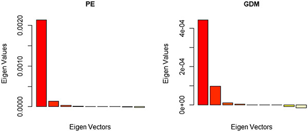
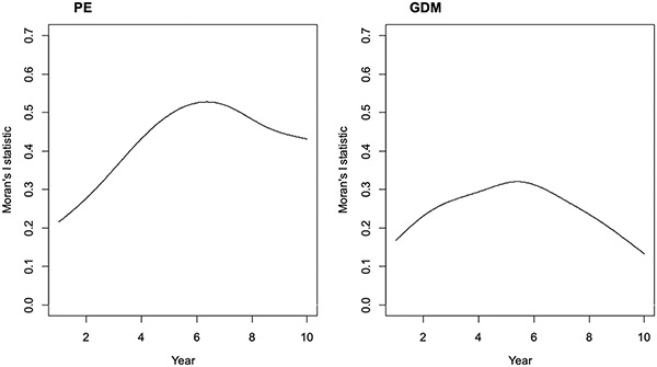
Functional Moran’s I statistics were shown in Table 2. The spatial-functional PCA revealed that there are clear global structures (positive in red) but little local structures (negative in yellow) as seen in Fig. 4. Spatial autocorrelation can be detected from the spatial-functional principal components which explain more than 95% of variability of both diseases’ incidences. Thus, a spatiotemporal model is necessary. The B-spline smoothed Moran’s I statistics (see Fig. 8 in Appendix A) showed that Moran’s I statistics reach their maximum in the year 2011 for both PE and GDM, indicating an evolution of spatial pattern over time.
Table 2.
Results from the functional Moran’s I tests
| sPCA | PE | GDM | ||||
|---|---|---|---|---|---|---|
| Moran’s I | p-value | Variability (%) | Moran’s I | p-value | Variability (%) | |
| 1st score positive | 0.623 | 0.001 | 91.44 | 0.43 | 0.001 | 75.98 |
| 2nd score positive | 0.307 | 0.001 | 5.71 | 0.354 | 0.001 | 16.96 |
| 3rd score positive | 0.125 | 0.049 | 1.46 | 0.182 | 0.01 | 2.17 |
| 1st score negative | −0.156 | 0.022 | 0.56 | −0.144 | 0.058 | 2.29 |
Fig. 4.
sPCA results of the smoothed yearly PE/GDM incidence rate
Model selection
The overall fit of the six spatiotemporal candidate models introduced above (using first trimester PM2.5 exposure) were displayed in Table 3. The smaller DIC and WAIC values suggested that the Leroux AR1 model and Leroux adaptive model fit the data better for both PE and GDM.
Table 3.
Model comparison criteria for six candidate models, fitted with cumulative PM2.5 exposure in first trimester
| PE | GDM | |||
|---|---|---|---|---|
| DIC | WAIC | DIC | WAIC | |
| Leroux-AR1 | 36752 | 36882 | 34300 | 34382 |
| Leroux-adaptive | 36734 | 36860 | 34284 | 34369 |
| Leroux-ANOVA | 37611 | 37617 | 35063 | 35092 |
| Leroux-separable spatial | 38570 | 38842 | 35877 | 36026 |
| BYM-linear | 38962 | 39028 | 36076 | 36126 |
| BYM-AR1 | 37647 | 37640 | 35084 | 35104 |
With further exploration on the local spatial structure in the adaptive models, no significant differences among the local spatial structures were identified. DIC differences between Leroux AR1 model and Leroux adaptive model were small. Thus, we chose the Leroux AR1 model as our final model.
Analytical results
Preeclampsia
To understand the effect of PM2.5 exposure, we evaluated the average exposure level during the first trimester, the second trimester, and during the first 6 months with three separate models. The three independent variables showed similar effects on PE. The results are displayed in Table 4.
Table 4.
Parameters of Leroux AR1 model—PE
| Model 1 | Model 2 | Model 3 | ||||
|---|---|---|---|---|---|---|
| RR | 95% CI | RR | 95% CI | RR | 95% CI | |
| PM2.5 on 1st trimester | 1.005 | 1.001–1.008 | ||||
| PM2.5 on 2nd trimester | 1.005 | 1.000–1.009 | ||||
| PM2.5 on first 6 months | 1.005 | 1.002–1.009 | ||||
| May to July | 1.048 | 1.022-1.076 | 1.062 | 1.035-1.090 | 1.055 | 1.030-1.082 |
After accounting for the spatiotemporal autocorrelation, PM2.5 exposure levels during the three time periods were either significantly or borderline significantly associated with PE risk. For the daily average PM2.5 exposure level during the first 6 months, one unit increase was associated with 0.5% increase in PE risk ratio. Conception during May to July was associated with 5.5% increase in PE risk ratio compared to other months.
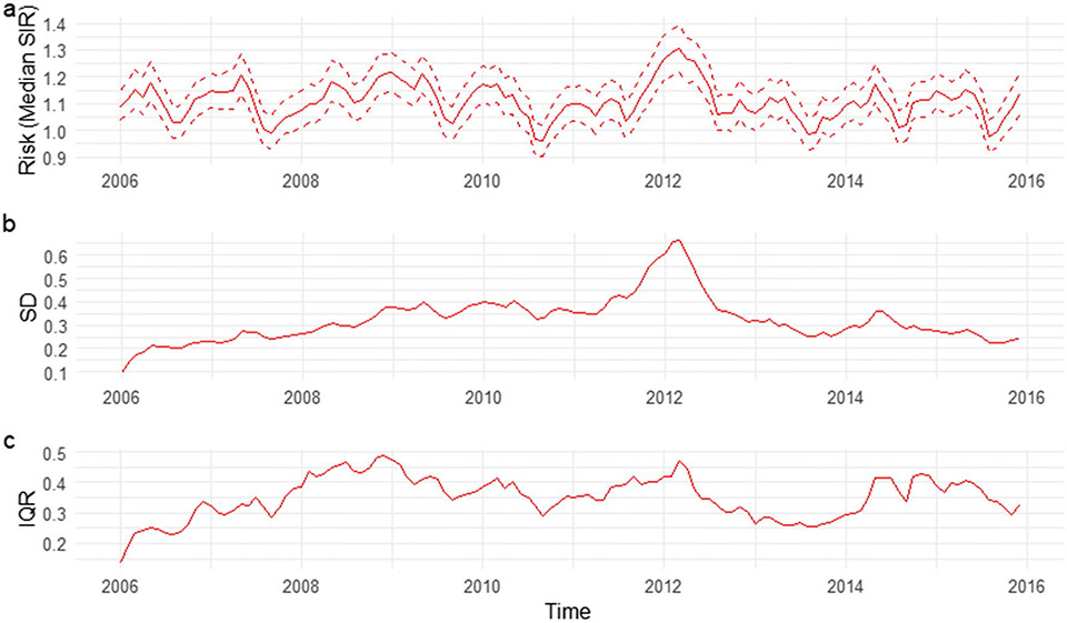
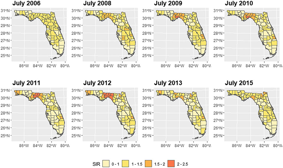
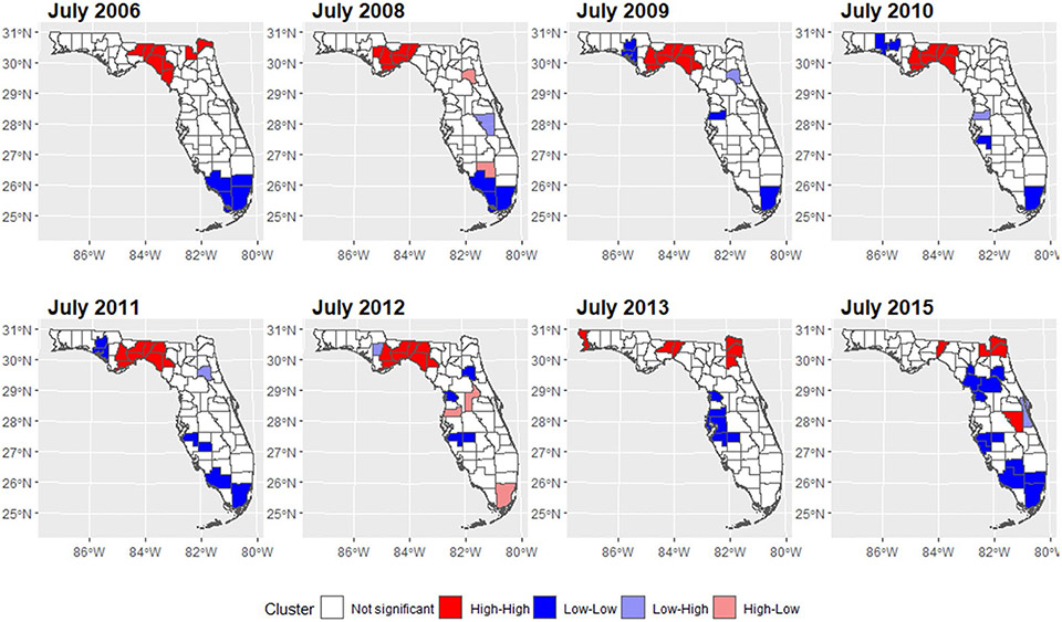
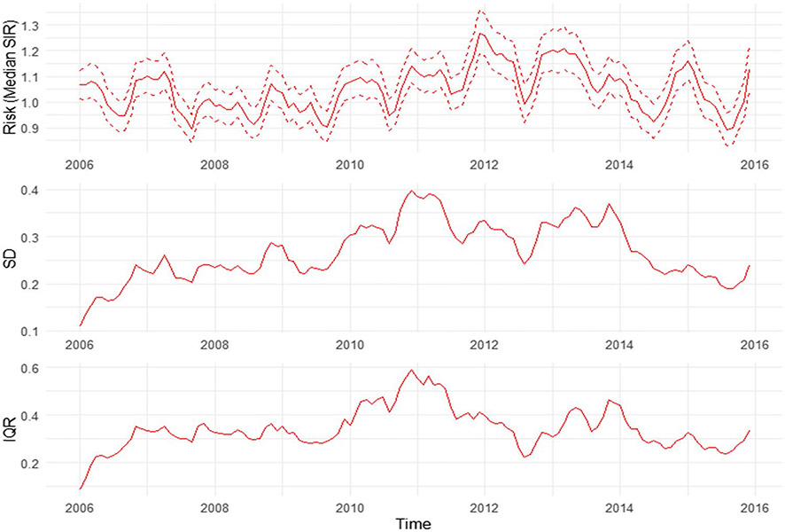
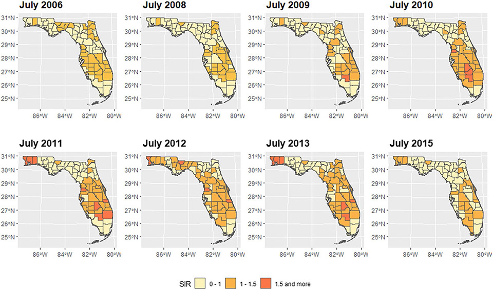
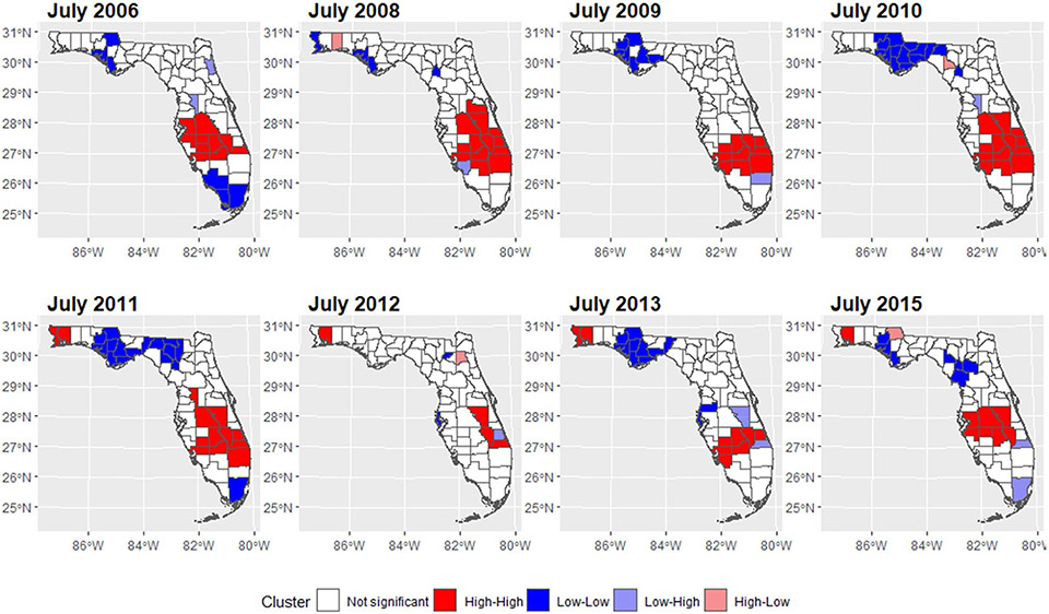
We mapped the smoothed SIR based on Model 3 for 8 random months. The estimated trend for PE risk was presented in Fig. 5. The SIR maps and LISA maps for selected months were plotted in Figs. 6 and 7. From these figures, it can be easily seen that the adjusted PE risk was stable with a peak in 2012, and spatial inequality, measured by standard deviation (SD) and interquartile range (IQR) of estimated risks increased slightly from 2006 to 2009, also reaching the summit in 2012. North Florida, especially Wakulla, Leon, and Jefferson Counties, were hotspots with relatively high PE risk, as they were identified as high-high clusters in the LISA map, meaning they were areas with high risk surrounded by areas of high risk. But the situation has been getting better since 2013. Duval County and its neighboring counties became the new hotspots. The striking surge of PE risk in Central North Florida around 2012 raises opportunities to identify unknown risk factors and is worth further investigation on comprehensive historical environmental data at this specific region.
Fig. 5.
Monthly smoothed risk and spatial inequality for PE in Florida from 2006 to 2015. a Median of estimated risk. b Standard deviation of estimated risk. c IQR of estimated risk
Fig. 6.
Maps of estimated PE SIR in Florida for selected months
Fig. 7.
Cluster maps of PE risk in Florida for selected months
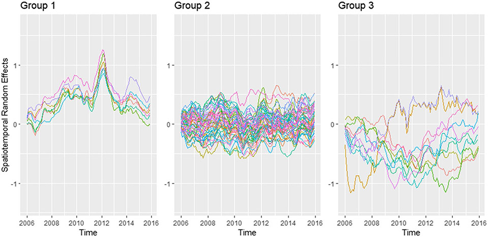
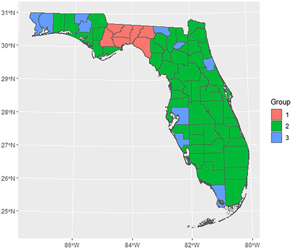
The random spatiotemporal effect for each county was plotted in Fig. 9 (see Appendix A). Each line represents a county. The pattern can be categorized into three groups based on the mean and variance. Group 1 (Gadsden, Jefferson, Leon, Liberty, Madison, Taylor, and Wakulla) has a striking peak around 2012, which should be the main cause of the increased median PE risk and spatial inequality at that time. Counties in group 3 (Escambia, Flagler, Hamilton, Hillsborough, Holmes, Monroe, Santa Rosa, Sarasota, Union, Washington) have larger variances while counties in group 2 have more stable spatiotemporal random effects. Spatial distribution of the three groups was represented in Fig. 10 (see Appendix A). Further analysis should be conducted in groups 1 and 3 counties to understand the reasons for that peak and large variance.
Gestational diabetes
Month indicator was not included in the GDM model, as it was not significant and did not affect the models’ performance. Like PE, the result from the Leroux AR1 model (Table 5) indicated significant positive association between PM2.5 levels during all three periods and GDM risk. One unit increase for daily average PM2.5 exposure in the first 6 months was associated with 4.0% increase in GDM risk ratio.
Table 5.
Parameters from Leroux AR1 model—GDM
| Model 1 | Model 2 | Model 3 | ||||
|---|---|---|---|---|---|---|
| RR | 95% CI | RR | 95% CI | RR | 95% CI | |
| PM2.5 on 1st trimester | 1.022 | 1.008–1.036 | ||||
| PM2.5 on 2nd trimester | 1.018 | 1.005–1.031 | ||||
| PM2.5 on first 6 months | 1.040 | 1.024–1.056 | ||||
The trend, spatial inequality, smoothed SIR, and LISA cluster maps were also plotted based on model 3 (see Figs. 11, 12, 13 in Appendix A). The GDM risk trend showed a similar pattern to the PE risk trend, with 2012 as the turning point. The spatial inequality increased at the beginning and then decreased since 2011. Central South Florida (clustered around Glades County) and Northwest Florida (clustered around Santa Rosa County) were experiencing relatively higher GDM risks. And the Gulf County at North Florida was cluster with lower GDM risks.
Discussion
The current study compared six spatiotemporal models with Bayesian approach and illustrated the different structures used for their spatial, temporal, and spatiotemporal terms. It can be used as a reference point for future applications. The application to the PE and GDM risk in Florida across a span of 10 years showed that Leroux AR1 model performed best in terms of accounting for the spatiotemporal trends presented, for both PE and GDM. According to Lee et al. (2018), the model is appropriate to estimate the evolution of the spatial random effects surface over time. This result is in accordance with the functional Moran’s I analysis result, which shows an evolution of spatial dependency. We cannot conclude which model is best in general, as each model has its advantages in certain scenarios.
To the best of our knowledge, this is the first study focusing on the spatiotemporal pattern of PE and GDM in Florida. This study confirmed the existence of spatial dependency in PE and GDM risks. The fitted maps demonstrated gradual spatial smoothing, providing stability to the visualization of areas of elevated risk for a relatively rare outcome at the spatial scale of counties. PE and GDM are the most common medical complications of pregnancy. They are frequently reported comorbidities as they are both characterized by oxidative stress and endothelial dysfunction (Guimarães et al. 2014; Karacay et al. 2010). PE and GDM showed similar risk trends and spatial inequality trends in this study. However, the spatial patterns were not the same. While the hot spot of PE was located in the North Central Florida, higher GDM risks were identified in the Central Florida and Northwest Florida. Through Leroux AR1 model, a spike of PE incidence was illustrated in North Central Florida including Leon County, Wakulla County, and their neighbors around 2012, suggesting that there are potential unmeasured risk factors. A better understanding of the mechanism for the detected high risk is necessary to design and implement public health interventions.
Our findings reinforced that neighborhood PM2.5 in ambient air pollution is significantly correlated with PE and GDM risk. The findings are scientifically conceivable because prior research linked perinatal exposure to PM2.5 to placental oxidative stress, hypercoagulability, inflammation, and thrombosis—all of which can lead to preeclampsia (Kannan et al. 2006; Saenen et al. 2017; Yi et al. 2017). Studies have shown that the pregnant women exposing to air pollutants can cause insulin resistance leading to hyperinsulinemia (Haberzettl et al. 2016). The primary standard for PM2.5 is 12 μg/m3. In Florida, the statewide annual average PM2.5 is lower than 10 μg/m3. The finding showed that even “safe” level exposure of PM2.5 would increase the risk of PE and GDM.
The association between PM2.5 exposure and disease risk were estimated in three time windows: the first trimester, the second trimester, and the first 6 months after conception (include both the first and second trimesters). A study suggested that the association between PM2.5 and GDM was strongest between weeks 7 and 18, which overlap the late first and early second trimesters (Miron-Celis et al. 2023). A meta-analysis found that both the first and second trimesters exposure of PM2.5 were associated with GDM risk, and the second trimester showed a stronger effect. In this study, the effect of average PM2.5 exposure in the first 6 months on GDM were more prominent compared to exposure level in the first or second trimester. PM2.5 effect on PE during the three time windows are similar with each other.
Even though PM2.5 level was associated with disease risk, the decreasing of air pollution level did not lead to decreased disease incidence risks. It may be because of the small magnitude of effect. According to a cohort research published by Lee, a 4 μg/m3 increase in PM2.5 exposure during the first trimester of pregnancy raised the incidence of PE by 15% (Lee et al. 2013). Furthermore, a meta-analysis revealed a 32% rise of PE risk for every 10 μg/m3 increase of PM2.5 exposure (Yu et al. 2020). According to our findings, the chance of developing a PE would rise by 0.5% for 1 μg/m3 increase of PM2.5 exposure, which is 5.1% for every 10 μg/m3 exposure increase. The magnitude of PM2.5 effect in this study is much smaller than previous claims. The difference is probably due to the different estimator of risks. In this study, disease risks were measured as SIR, which is the number of disease cases over the number of expected cases. The previous studies discussed above normally use odds ratio, that can exaggerate the relative risk, especially when the probability of disease is not rare (Grimes and Schulz 2008).
This study covered 10 years and 67 Florida counties, with large representative population. We confirmed PM2.5 in ambient air was a risk factor for PE and GDM, in all the three exposure windows. Both the smoothed risks and the spatial inequalities for the two pregnancy complications were high in 2011–2012. Several high-risk clusters were identified. Limitations in this study were mainly due to data restriction. Preeclampsia and gestational hypertension were not divided. Even though we adjusted for common risk factors such as race, ethnicity, age, and BMI, there were other factors for PE and GDM that should be considered, such as socioeconomic status and occupation. Further studies controlling for these covariates are needed. In-depth investigations on Central North Florida counties between 2011 and 2013 should be conducted to understand the unknown reasons for the increased PE risk.
Conclusion
This study analyzed the spatial and temporal patterns of PE and GDM in Florida from 2006 to 2015 with six spatiotemporal models, provided valuable insights into the dynamic distribution of these two conditions at the county level and identified areas of elevated risk. The study confirmed the existence of positive spatial dependencies of PE and GDM in Florida, indicating the necessity to implement public health interventions in certain areas. It also detected a spike of preeclampsia incidence in North Florida around 2011, suggesting a chance to capture unidentified risk factors. The study highlighted the significant association between neighborhood PM2.5 air pollution and the risk of PE and GDM, even when PM2.5 levels are below the standard. It is imperative to persist in the endeavors at mitigating air pollution.
Acknowledgements
The authors would like to thank the FL-DOH for providing the data and acknowledge that the findings and conclusions are those of the authors and do not necessarily represent the official position of the Florida Department of Health.
Funding
This work is supported by The National Heart Lung and Blood Institute (Grant number: K01 HL146944).
Abbreviations
- AR1
first order autoregressive
- BHM
Bayesian hierarchical model
- BMI
body mass index
- CAR
conditional autoregressive
- DIC
deviance information criterion
- GDM
gestational diabetes mellitus
- IQR
interquartile range
- LISA
local indicators of spatial association
- PE
preeclampsia
- SD
standard deviation
- SIR
standardized incidence ratio
- WAIC
widely applicable information criterion
Appendix
Fig. 8.
Functional Moran’s I statistics
Fig. 9.
Spatiotemporal random effects in FL counties. Grouped by mean and variance. Based on Leroux-AR1 (PE) model
Fig. 10.
Map of spatiotemporal random effect groups. Based on Leroux-AR1 (PE) model
Fig. 11.
Monthly smoothed risk and spatial inequality for GDM in Florida from 2006 to 2015. a Median of estimated risk. b Standard deviation of estimated risk. c IQR of estimated risk
Fig. 12.
Maps of estimated GDM SIR in Florida for selected months
Fig. 13.
Cluster maps of GDM risk in Florida for selected months
Footnotes
Ethical approval This study is approved with FIU IRB-20-0033.
Consent to participate Informed consent was obtained from all subjects involved in the study by Florida Department of Health.
Consent for publication Informed consent was obtained from all subjects involved in the study by Florida Department of Health.
Competing interests The authors declare no competing interests. Findings and conclusions are those of the authors and do not necessarily represent the official position of the Florida Department of Health.
Data availability
Data use approval is needed from the Florida Department of Health.
References
- Anderson C, Lee D, Dean N (2017) Spatial clustering of average risks and risk trends in Bayesian disease mapping. Biom J 59(1):41–56. 10.1002/bimj.201600018 [DOI] [PubMed] [Google Scholar]
- Bernardinelli L, Clayton D, Pascutto C, Montomoli C, Ghislandi M, Songini M (1995) Bayesian analysis of space-time variation in disease risk. Stat Med 14(21–22):2433–2443. 10.1002/sim.4780142112 [DOI] [PubMed] [Google Scholar]
- Besag J, York J, Mollié A (1991) Bayesian image restoration, with two applications in spatial statistics. Ann Inst Stat Math 43:1–20. 10.1007/BF00116466 [DOI] [Google Scholar]
- Billet S, Garçon G, Dagher Z, Verdin A, Ledoux F, Cazier F, Courcot D, Aboukais A, Shirali P (2007) Ambient particulate matter (PM2.5): physicochemical characterization and metabolic activation of the organic fraction in human lung epithelial cells (A549). Environ Res 105(2):212–223. 10.1016/j.envres.2007.03.001 [DOI] [PubMed] [Google Scholar]
- Brooks SP, Gelman A (1998) General methods for monitoring convergence of iterative simulations. J Comput Graph Stat 7(4):434–455. 10.1080/10618600.1998.10474787 [DOI] [Google Scholar]
- Buchanan TA, Xiang AH, Page KA (2012) Gestational diabetes mellitus: risks and management during and after pregnancy. Nat Rev Endocrinol 8(11):639–649. 10.1038/nrendo.2012.96 [DOI] [PMC free article] [PubMed] [Google Scholar]
- Casagrande SS, Linder B, Cowie CC (2018) Prevalence of gestational diabetes and subsequent type 2 diabetes among U.S. women. Diabetes Res Clin Pract 141:200–208. 10.1016/j.diabres.2018.05.010 [DOI] [PubMed] [Google Scholar]
- Cramb SM, Moraga P, Mengersen KL et al. (2017) Spatial variation in cancer incidence and survival over time across Queensland, Australia. Spat Spatio Temp Epidemiol 23:59–67. 10.1016/j.sste.2017.09.002 [DOI] [PubMed] [Google Scholar]
- Daniel S, Kloog I, Factor-Litvak P, Levy A, Lunenfeld E, Kioumourtzoglou M (2021) Risk for preeclampsia following exposure to PM2.5 during pregnancy. Environ Int 156:106636. 10.1016/j.envint.2021.106636 [DOI] [PubMed] [Google Scholar]
- DeSisto CL, Kim SY, Sharma AJ (2014) Prevalence estimates of gestational diabetes mellitus in the United States, Pregnancy Risk Assessment Monitoring System (PRAMS), 2007-2010. Prev Chronic Dis 11:E104. 10.5888/pcd11.130415 [DOI] [PMC free article] [PubMed] [Google Scholar]
- Di Q, Amini H, Shi L, Kloog I, Silvern R, Kelly J, Sabath MB, Choirat C, Koutrakis P, Lyapustin A, Wang Y, Mickley LJ, Schwartz J (2019) An ensemble-based model of PM2.5 concentration across the contiguous United States with high spatiotemporal resolution. Environ Int 130:104909. 10.1016/j.envint.2019.104909 [DOI] [PMC free article] [PubMed] [Google Scholar]
- Di Q, Wei Y, Shtein A, Hultquist C, Xing X, Amini H, Shi L, Kloog I, Silvern R, Kelly JT, Sabath MB, Choirat C, Koutrakis P, Lyapustin A, Wang Y, Mickley LJ (2021) Daily and annual PM2.5 concentrations for the contiguous United States, 1-km grids, v1 (2000-2016). In: NASA Socioeconomic Data and Applications Center (SEDAC). 10.7927/0rvr-4538 [DOI] [Google Scholar]
- Duley L (2009) The global impact of pre-eclampsia and eclampsia. Semin Perinatol. 10.1053/j.semperi.2009.02.010 [DOI] [PubMed] [Google Scholar]
- Duncan EW, White NM, Mengersen K (2017) Spatial smoothing in Bayesian models: a comparison of weights matrix specifications and their impact on inference. Int J Health Geogr 33(3):130–137. 10.1186/s12942-017-0120-x [DOI] [PMC free article] [PubMed] [Google Scholar]
- Fox R, Kitt J, Leeson P, Aye CYL, Lewandowski AJ (2019) Preeclampsia: risk factors, diagnosis, management, and the cardiovascular impact on the offspring. J Clin Med 8(10):1625. 10.3390/jcm8101625 [DOI] [PMC free article] [PubMed] [Google Scholar]
- Gelman A, Rubin DB (1992) Inference from iterative simulation using multiple sequences. Stat Sci 7(4):457–472. 10.1214/ss/1177011136 [DOI] [Google Scholar]
- Getis A (2010) Spatial Autocorrelation. In: Fischer MM, Getis A (eds) Handbook of applied spatial analysis: software tools, methods and applications. Springer, Berlin Heidelberg, Berlin, Heidelberg, pp 255–278 [Google Scholar]
- Griffith DA (2009) Spatial Autocorrelation. In: Kitchin R, Thrift N (eds) International Encyclopedia of Human Geography. Elsevier, Oxford, pp 308–316 [Google Scholar]
- Grimes DA, Schulz KF (2008) Making sense of odds and odds ratios. Obstet Gynecol 111(2 Pt 1):423–426. 10.1097/01.AOG.0000297304.32187.5d [DOI] [PubMed] [Google Scholar]
- Guimarães MF, Brandão AH, Rezende CA, Cabral AC, Brum AP, Leite HV, Capuruço CA (2014) Assessment of endothelial function in pregnant women with preeclampsia and gestational diabetes mellitus by flow-mediated dilation of brachial artery. Arch Gynecol Obstet 290(3):441–447. 10.1007/s00404-014-3220-x [DOI] [PubMed] [Google Scholar]
- Haberzettl P, O'Toole TE, Bhatnagar A, Conklin DJ (2016) Exposure to fine particulate air pollution causes vascular insulin resistance by inducing pulmonary oxidative stress. Environ Health Perspect 124(12):1830–1839. 10.1289/EHP212 [DOI] [PMC free article] [PubMed] [Google Scholar]
- Hassan AA (2021) Spatial data analysis : applications to population health. Statistics [math.ST]. Université de Lille. English. NNT : 2021LILUB021. https://theses.hal.science/tel-03685200/document [Google Scholar]
- Hu C, Gao X, Fang Y, Jiang W, Huang K, Hua X, Yang X, Chen H, Jiang Z, Zhang X (2020) Human epidemiological evidence about the association between air pollution exposure and gestational diabetes mellitus: systematic review and meta-analysis. Environ Res 180:108843. 10.1016/j.envres.2019.108843 [DOI] [PubMed] [Google Scholar]
- Kannan S, Misra DP, Dvonch JT, Krishnakumar A (2006) Exposures to airborne particulate matter and adverse perinatal outcomes: a biologically plausible mechanistic framework for exploring potential effect modification by nutrition. Environ Health Perspect 114(11):1636–1642. 10.1289/ehp.9081 [DOI] [PMC free article] [PubMed] [Google Scholar]
- Karacay Ö, Sepici-Dincel A, Karcaaltincaba D, Sahin D, Yalvaç S, Akyol M, Kandemir Ö, Altan N (2010) A quantitative evaluation of total antioxidant status and oxidative stress markers in preeclampsia and gestational diabetic patients in 24–36 weeks of gestation. Diabetes Res Clin Pract 89(3):231–238. 10.1016/j.diabres.2010.04.015 [DOI] [PubMed] [Google Scholar]
- Knorr-Held L (2000) Bayesian modelling of inseparable space-time variation in disease risk. Stat Med 19(17–18):2555–2567. [DOI] [PubMed] [Google Scholar]
- Kottas A, Duan JA, Gelfand AE (2008) Modeling disease incidence data with spatial and spatio temporal dirichlet process mixtures. Biom J 50(1):29–42. 10.1002/bimj.200610375 [DOI] [PubMed] [Google Scholar]
- Lawson AB (2018) Bayesian disease mapping: hierarchical modeling in spatial epidemiology. CRC press [Google Scholar]
- Lee D, Rushworth A, Napier G (2018) Spatio-temporal areal unit modeling in r with conditional autoregressive priors using the CARBayesST package. J Stat Softw 84:1–39. 10.18637/jss.v084.i0930450020 [DOI] [Google Scholar]
- Lee P, Roberts JM, Catov JM, Talbott EO, Ritz B (2013) First trimester exposure to ambient air pollution, pregnancy complications and adverse birth outcomes in Allegheny County, PA. Matern Child Health J 17(3):545–555. 10.1007/s10995-012-1028-5 [DOI] [PMC free article] [PubMed] [Google Scholar]
- Leroux BG, Lei X, Breslow N (2000) Estimation of disease rates in small areas: a new mixed model for spatial dependence. In: Halloran ME, Berry D (eds) Statistical Models in Epidemiology, the Environment, and Clinical Trials. Springer, New York, NY. 10.1007/978-1-4612-1284-3_4 [DOI] [Google Scholar]
- MacNab YC (2022) Bayesian disease mapping: past, present, and future. Spat Stat 50:100593. 10.1016/j.spasta.2022.100593 [DOI] [PMC free article] [PubMed] [Google Scholar]
- MacNab YC, Dean CB (2001) Autoregressive spatial smoothing and temporal spline smoothing for mapping rates. Biometrics 57(3):949–956. 10.1111/j.0006-341x.2001.00949.x [DOI] [PubMed] [Google Scholar]
- Miron-Celis M, Talarico R, Villeneuve PJ, Crighton E, Stieb DM, Stanescu C, Lavigne É (2023) Critical windows of exposure to air pollution and gestational diabetes: assessing effect modification by maternal pre-existing conditions and environmental factors. Environ Health 22(1):26. 10.1186/s12940-023-00974-z [DOI] [PMC free article] [PubMed] [Google Scholar]
- Napier G, Lee D, Robertson C, Lawson A, Pollock KG (2016) A model to estimate the impact of changes in MMR vaccine uptake on inequalities in measles susceptibility in Scotland. Stat Methods Med Res 25(4):1185–1200. 10.1177/0962280216660420 [DOI] [PubMed] [Google Scholar]
- Orozco-Acosta E, Adin A, Ugarte MD (2023) Big problems in spatiotemporal disease mapping: methods and software. Comput Methods Prog Biomed 231:107403. 10.1016/j.cmpb.2023.107403 [DOI] [PubMed] [Google Scholar]
- Rioux C, Grandbastien B, Astagneau P (2006) The standardized incidence ratio as a reliable tool for surgical site infection surveillance. Infect Control Hosp Epidemiol 27(8):817–824. 10.1086/506420 [DOI] [PubMed] [Google Scholar]
- Rohr Thomsen C, Brink Henriksen T, Uldbjerg N, Milidou I (2020) Seasonal variation in the hypertensive disorders of pregnancy in Denmark. Acta Obstet Gynecol Scand 99(5):623–630. 10.1111/aogs.13786 [DOI] [PubMed] [Google Scholar]
- Rue H, Martino S, Chopin N (2009) Approximate Bayesian inference for latent Gaussian models by using integrated nested Laplace approximations. J R Stat Soc, B: Stat Methodol 71(2):319–392. 10.1111/j.1467-9868.2008.00700.x [DOI] [Google Scholar]
- Rushworth A, Lee D, Mitchell R (2014) A spatio-temporal model for estimating the long-term effects of air pollution on respiratory hospital admissions in Greater London. Spat Spatiotemporal Epidemiol 10:29–38. 10.1016/j.sste.2014.05.001 [DOI] [PubMed] [Google Scholar]
- Rushworth A, Lee D, Sarran C (2017) An adaptive spatiotemporal smoothing model for estimating trends and step changes in disease risk. J R Stat Soc, C: Appl Stat 66(1):141–157. 10.1111/rssc.12155 [DOI] [Google Scholar]
- Saenen ND, Vrijens K, Janssen BG, Roels HA, Neven KY, Vanden Berghe W, Gyselaers W, Vanpoucke C, Lefebvre W, De Boever P (2017) Lower placental leptin promoter methylation in association with fine particulate matter air pollution during pregnancy and placental nitrosative stress at birth in the ENVIR ON AGE cohort. Environ Health Perspect 125(2):262–268. 10.1289/EHP38 [DOI] [PMC free article] [PubMed] [Google Scholar]
- Sławek-Szmyt S, Kawka-Paciorkowska K, Ciepłucha A, Lesiak M, Ropacka-Lesiak M (2022) Preeclampsia and fetal growth restriction as risk factors of future maternal cardiovascular disease-a review. J Clin Med 11(20):6048. 10.3390/jcm11206048 [DOI] [PMC free article] [PubMed] [Google Scholar]
- Tang X, Zhou J, Luo F, Han Y, Heianza Y, Cardoso MA, Qi L (2020) Air pollution and gestational diabetes mellitus: evidence from cohort studies. BMJ Open Diabetes Res Care 8(1):e000937. 10.1136/bmjdrc-2019-000937 [DOI] [PMC free article] [PubMed] [Google Scholar]
- Ugarte MD, Adin A, Goicoa T (2017) One-dimensional, two-dimensional, and three dimensional B-splines to specify space–time interactions in Bayesian disease mapping: model fitting and model identifiability. Spat Stat 22:451–468. 10.1016/j.spasta.2017.04.002 [DOI] [Google Scholar]
- Verburg PE, Dekker GA, Tucker G, Scheil W, Erwich JJHM, Roberts CT (2018) Seasonality of hypertensive disorders of pregnancy-a South Australian population study. Pregnancy Hypertens 12:118–123. 10.1016/j.preghy.2018.04.006 [DOI] [PubMed] [Google Scholar]
- Waller LA, Carlin BP (2010) Disease mapping. Chapman Hall CRC Handb Mod Stat Methods 2010:217–243. 10.1201/9781420072884-c14 [DOI] [PMC free article] [PubMed] [Google Scholar]
- Weinberg CR, Shi M, Basso O, DeRoo LA, Harmon Q, Wilcox AJ, Skjærven R (2017) Season of conception, smoking, and preeclampsia in Norway. Environ Health Perspect 125(6):067022. 10.1289/EHP963 [DOI] [PMC free article] [PubMed] [Google Scholar]
- Yi L, Wei C, Fan W (2017) Fine-particulate matter (PM2.5), a risk factor for rat gestational diabetes with altered blood glucose and pancreatic GLUT2 expression. Gynecol Endocrinol 33(8):611–616. 10.1080/09513590.2017.1301923 [DOI] [PubMed] [Google Scholar]
- Yin P, Mu L, Madden M et al. (2014) Hierarchical Bayesian modelling of spatio-temporal patterns of lung cancer incidence risk in Georgia, USA: 2000–2007. J Geogr Syst 16:387–407. 10.1007/s10109-014-0200-4 [DOI] [Google Scholar]
- Yu H, Yin Y, Zhang J, Zhou R (2020) The impact of particulate matter 2.5 on the risk of preeclampsia: an updated systematic review and meta-analysis. Environ Sci Pollut Res Int 27(30):37527–37539. 10.1007/s11356-020-10112-8 [DOI] [PMC free article] [PubMed] [Google Scholar]
- Zhang Y, Wang J, Chen L, Yang H, Zhang B, Wang Q, Hu L, Zhang N, Vedal S, Xue F, Bai Z (2019) Ambient PM2.5 and clinically recognized early pregnancy loss: a case-control study with spatiotemporal exposure predictions. Environ Int 126:422–429. 10.1016/j.envint.2019.02.062 [DOI] [PubMed] [Google Scholar]
- Zhou X, Lin H (2008) Spatial Weights Matrix. In: Shekhar S, Xiong H (eds) Encyclopedia of GIS. Springer, US, Boston, MA, p 1113 [Google Scholar]
Associated Data
This section collects any data citations, data availability statements, or supplementary materials included in this article.
Data Availability Statement
Data use approval is needed from the Florida Department of Health.


