A simple neural network model of the hippocampus suggesting its pathfinding role in episodic memory retrieval

Abstract

The goal of this work is to extend the theoretical understanding of the relationship between hippocampal spatial and memory functions to the level of neurophysiological mechanisms underlying spatial navigation and episodic memory retrieval. The proposed unifying theory describes both phenomena within a unique framework, as based on one and the same pathfinding function of the hippocampus. We propose a mechanism of reconstruction of the context of experience involving a search for a nearly shortest path in the space of remembered contexts. To analyze this concept in detail, we define a simple connectionist model consistent with available rodent and human neurophysiological data. Numerical study of the model begins with the spatial domain as a simple analogy for more complex phenomena. It is demonstrated how a nearly shortest path is quickly found in a familiar environment. We prove numerically that associative learning during sharp waves can account for the necessary properties of hippocampal place cells. Computational study of the model is extended to other cognitive paradigms, with the main focus on episodic memory retrieval. We show that the ability to find a correct path may be vital for successful retrieval. The model robustly exhibits the pathfinding capacity within a wide range of several factors, including its memory load (up to 30,000 abstract contexts), the number of episodes that become associated with potential target contexts, and the level of dynamical noise. We offer several testable critical predictions in both spatial and memory domains to validate the theory. Our results suggest that (1) the pathfinding function of the hippocampus, in addition to its associative and memory indexing functions, may be vital for retrieval of certain episodic memories, and (2) the hippocampal spatial navigation function could be a precursor of its memory function.

The phenomenon of hippocampal spatial representations and the hippocampal role in episodic memory retrieval remain two of the most puzzling mysteries in cognitive neuroscience that intuitively seem to be connected to each other. Since the finding that the hippocampus plays a pivotal role in long-term memory consolidation (Scoville and Milner 1957; Zola-Morgan and Squire 1986), many proposals have been made regarding its specific role (Teyler and Discenna 1985; Squire 1987; O'Reilly and McClelland 1994; McClelland et al. 1995). A prominent view of the mechanisms underlying consolidation of episodic memories involves fast formation (e.g., via Hebbian mechanisms) of strong associations between hippocampal sparse patterns of activity and distributed neocortical representations. As a result, the former subsequently serve as pointers to the latter. This memory-indexing theory that goes back to Teyler and Discenna (1985, 1986) and underlies several subsequent major theoretical contributions to the field (Nadel and Moscovitch 1997, 2001; Wheeler et al. 1997; Tulving 2002) assumes that a memory of an episode is retrieved by reactivating a hippocampal pointer to it. Consistent with this view, recent clinical and fMRI studies indicate that the hippocampus in humans is involved in and required for retrieval of all autobiographical, but not semantic memories (Vargha-Khadem et al. 1997; Ryan et al. 2001; Westmacot et al. 2001; Maguire and Frith 2003).

At the same time, details of this picture remain unclear. In order to retrieve (and make sense of) an episodic memory, it is necessary to reconstruct contextual information that was present at the time of encoding. For some episodic memories, the vital contextual information may not be explicitly encoded in memory traces or their associations. Consider the following example. An idea of driving under a building may never come to your mind while planning a way home, because you know that this is impossible. Your decision making is influenced by this knowledge, while on the other hand, you are not aware of this knowledge at the time of decision making, and therefore, you will not remember it in association with the episode. This knowledge, however, may not be in effect in the future when a tunnel is built. From the future context point of view, your episodic memory of driving home acquired before the construction began may seem irrational, and therefore, hard to retrieve without reinstating the context of the past. According to Moscovitch and Melo (1997), episodic memory traces lack their historical context (e.g., time stamps), but may include associative context (which refers to the multimodal, e.g., spatial background that comprises the event). Therefore, strategic retrieval (as opposed to cued recall) of an episodic memory may require reconstruction of the original context of experience step by step via effortful, guided memory search that is controlled by the prefrontal cortex (PFC) (Moscovitch 1989, 1992; Moscovitch and Melo 1997; Fletcher and Henson 2001). The role of PFC in this process amounts to cue specification, strategic search, maintenance, monitoring, and verification of retrieved information, while medial temporal lobe cortices (MTL) and the hippocampus may play the role of pattern completion and comparison (Simons and Spiers 2003). Experimental data confirm the idea that the hippocampus is essentially involved in the process of contextual reinstatement (e.g., Dobbins et al. 2003). Its particular functional role in this process is currently hotly debated in computational modeling studies (e.g., Howard and Kahana 2002; Becker and Lim 2003).

On the other hand, hippocampal memory function must be reconciled with the spatial semantics of hippocampal activity patterns, which have been intensively studied for more than three decades. The rodent hippocampus is known to represent spatial maps of environments. Hippocampal pyramidal cells, called place cells in rodents, each selectively fire at a high rate when the animal is located in a particular spatial domain, called a place field of the place cell. This type of firing is observed during active maze running (O'Keefe and Dostrovsky 1971), and to some extent, during slow-wave sleep states (Wilson and McNaughton 1994; Jarosiewicz et al. 2002; Lee and Wilson 2002; Jarosiewicz and Skaggs 2004). Equivalent or similar phenomena were observed in primates (Rolls and O'Mara 1995; Robertson et al. 1998), including humans (Ekstrom et al. 2003). The system of place fields forms a cognitive map of an environment (O'Keefe and Nadel 1978, 1979). Although hippocampal cognitive maps have been implicated in navigation and in formation of episodic memories (for review, see Redish 1999), many basic questions about underlying mechanisms and place field semantics remain unanswered. For example, what are the general principles of place field formation? Why do they come in various shapes and sizes and typically have broad tails? How can a cognitive map be used for navigation if its activity during maze running only provides information about the current location? Alternatively, what exactly do place fields encode? Several theoretical frameworks have been proposed to answer these questions, including local view models (e.g., Burgess and O'Keefe 1996), path integration models (McNaughton 1996; McNaughton et al. 1996; Redish and Touretzky 1997), and trajectory learning models (e.g., Blum and Abbott 1996). None of the proposed solutions seem to answer all questions.

It has long been noticed that the combination of the two apparently different functions in one brain structure poses a great challenge in theoretical neuroscience. The metaphoric analogy between linking remembered episodes by context and linking nearby locations in an environment (e.g., Wallenstein et al. 1998) characterizes the present level of understanding of this issue, although several more specific proposals were put forward (Levy 1996; Recce and Harris 1996; Gaffan 1998; Robertson et al. 1998; Burgess 2002). A common ground in these proposals is the notion of a hippocampal pointer providing necessary associations. In the present study, we construct a model of episodic memory retrieval, departing from a traditional assumption that reactivating a hippocampal pointer is sufficient for retrieval of the associated episodic memory. Our assumption is that an episodic memory trace may not be retrievable without reinstatement of a missing contextual key—a key that is not associated with the pointer. We propose a theory explaining how this key is found by the hippocampus, why finding it may be impossible without the hippocampus, and how this relates to spatial navigation. Specifically, we show, using numerical simulations, that one and the same mechanism can work for episodic memory retrieval and for spatial navigation. We take this observation as the basis for a conceptual unification of the two hippocampal functions.

The central idea of the proposed approach can be unfolded as follows. Because the context of the retrieval conditions may be substantially different from the context of the remembered episode, the system must “prepare itself” for retrieval by reinstating vital contextual information that is not referenced in the target episode. This information needs to be acquired from a set of other episodic memories that serve as a key for understanding the target episode. This acquisition can be subserved by the system taking a quick path through the key set, briefly reactivating necessary memories one by one. Finding a correct path may be crucial for a successful retrieval. How can one decide which path is “correct”? In this study, we say that there is a connection from episodic memory A to episodic memory B, if, given an explicit awareness and an understanding of A, the system is capable of immediate retrieval and understanding of B without consulting any additional episodic knowledge (in contrast, available semantic knowledge may be used). Then, a rule that ensures the retrieval of an episodic memory X, given an initial state of awareness Y, is to follow a connected path from Y to X, i.e., a continuous path composed of relevant remembered episodes and connections among them.

One can think of a set of episodic memories and their connections as an abstract graph. Most of the content of episodic memories can be excluded from this model; nodes of the graph can be considered as pointers that merely label the essential context of remembered episodes. The connections of this graph may involve acts of imagination or assumption, perspective shifting, dropping or accepting various rules and conditions, etc. This interpretation is consistent with the view that episodic memories are reconstructed based on schemas rather than retrieved as images (e.g., Watkins and Gardner 1979; Parkin 1993; Moscovitch and Melo 1997; Schacter 1999; Rusted et al. 2000). The generalized notion of a cognitive map (O'Keefe and Nadel 1978) viewed as an abstract cognitive space, or a cognitive graph (Muller et al. 1996), or an internal cognitive model (Samsonovich and McNaughton 1997) can be understood as a set containing all previously explored contexts (no matter how abstract or specific they are) along with connections among them (understood in the above sense). Here, by an abstract context, we refer to a set of rules and facts that apply to a class of possible situations (McCarthy and Buvac 1997). Therefore, a given abstract context may specify a large set of episodic memories, yet it may be represented by one node in the graph (and accordingly, by one hippocampal pointer). Looking ahead, in our model, each CA1 unit will represent one such abstract context.

With this setup, considerations of efficiency of an episodic memory system inspire several conjectures. (1) It is reasonable to memorize available connections, at least a sufficient subset of them, in association with each remembered context or episode. (2) The resultant graph must be highly interconnected, in the sense that any shortest path in it has a limited, reasonably small length (measured as the number of connections), despite the huge size of the whole memory space (Alon 2003; Barabasi and Bonabeau 2003). An abstract example demonstrating this possibility is the space of 4.3·10¹⁹ states of Rubik's cube, where any shortest path involves no more than 20 moves, and each state offers only 12 possible moves. (3) A selected path in the graph must be among the shortest or nearly shortest paths. (4) Episodic memory system must be able to quickly find a nearly shortest path, given available connections, which makes its function closely related to that of a spatial navigation device. Our model assigns the pathfinding function to the hippocampus in addition to its other, better-known cognitive map functions (including multimodal associations, episodic memory indexing, and spatial self-representation). Validation of this proposal involves (1) analysis of experimental data supporting the mathematical model; (2) formalization of the concept outlined above in terms of the model; and (3) numerical application of the model to spatial, problem-solving, and episodic memory-retrieval paradigms selected to demonstrate the concept in action.

Connectivity in Cornu Ammonis

Cornu Ammonis (CA), or the hippocampus proper, consists of areas CA1–CA3. The principal neurons in CA areas are known as pyramidal cells (based on the shape of their somata), complex spike cells (based on their activity pattern), or place cells (based on their behavioral correlates). There are ∼3 × 10⁵ pyramidal cells in CA3 and 4 × 10⁵ in CA1 (Amaral et al. 1990). Multiunit recordings in freely behaving rats (Wilson and McNaughton 1993) show the following essential details. (1) Relative anatomical location of place cells does not correlate with their spatial preferences (Redish et al. 2001). (2) Approximately 0.1% of all CA3 pyramidal cells and ∼1% of all CA1 pyramidal cells are active at any given location in an environment (McNaughton et al. 1996). Accordingly, place fields in CA1 are typically bigger than in CA3. (3) Any given CA3 or CA1 pyramidal cell has a probability of about 30% to exhibit activity within a given environment (McNaughton et al. 1996). Typically, this activity is spatially selective (compact place field); nevertheless, it can be spontaneously exhibited at any location in the environment (broad “tails” and background noise). The other 70% of cells, however, may remain silent for the whole recording session.

A typical CA3 pyramidal cell is innervated by ∼12,000 other CA3 pyramidal cells (Ishizuka et al. 1990; Amaral and Witter 1995) via wide-spread projections (the axonal field of each cell covers ∼1/3 of the hippocampus) (Miles et al. 1988). A typical CA1 pyramidal cell is innervated by ∼16,000 CA3 pyramidal cells via Schaffer collaterals and commissural pathways (Bernard and Wheal 1994). These diffuse projections distributed throughout CA1 in a gradient fashion constitute the main input to CA1. In addition, both CA3 and CA1 areas receive diffuse input from the entorhinal cortex (which, in the case of CA3, is partially mediated by the dentate gyrus, DG). The main output of CA1 consists of topographically organized projections to the entorhinal cortex, both directly and through the subicular complex. The entorhinal cortex, in turn, has distributed two-way connections throughout the neocortex. Associative plasticity in CA1 appears to be crucial for memory consolidation (Shimizu et al. 2000).

Sharp waves and associative spatial learning

Sharp waves and ripples are high-frequency oscillatory events (lasting on average ∼100 msec) of nearly synchronous firing of many hippocampal place cells, accompanied by a temporary decrease or disappearance of the θ rhythm (O'Keefe and Nadel 1978; Buzsaki 1986; Sik et al. 1994). During typical behavioral experiments, rats exploring a maze do not run continuously (Fig. 1A). Rather, they intermittently pause, with a transient change in the hippocampal activity from θ mode to large-amplitude irregular activity (LIA), during which sharp waves and ripples are observed (Fig. 1A–C).

Figure 1.

Firing properties of place cells (see Supplemental online material at http://www.krasnow.gmu.edu/ascoli/sa_lm05_som/ for a color version of this figure). (A–C) CA1 firing patterns during a typical recording session of a rat running a maze (based on data from Kudrimoti et al. 1999, courtesy of B.L. McNaughton). The entire trajectory of the freely behaving rat (A) follows the rectangular apparatus, which is approximately one meter long. (B, C) Scatter plot of vertically arranged spikes (black pixels) of 28 simultaneously recorded cells from the same animal. The superimposed light background waveform shows the EEG. Horizontal dashes mark seconds (total duration of the session was 23 min, of which only two short intervals are shown). Narrow vertical columns of spikes marked by light-gray arrows are the sharp waves. (D–E) Phase precession in rat CA1 pyramidal cell firing, based on the data used and referenced in Samsonovich and McNaughton 1997, courtesy of B.L. McNaughton. (D, linear motion, E, random two-dimensional foraging) Grayscale-coded distribution of CA1 firing rates on a chart (defined in Samsonovich and McNaughton 1997), separated by phases of the θ rhythm and averaged in rat egocentric coordinates over the whole trajectory of the rat. The dark shade color corresponds to low, medium shade to medium, and light shade to high activity of CA1 place cells; uniform gray background corresponds to data missing due to extremely low activity in that area. The length of the arrow in each panel is 15 cm, its rear end is just behind the ears of the rat. Dials in top, right corners show the selected phase of the θ rhythm (the maximum of firing generally corresponds to the trough of the EEG). (F) Schematic representation of a possible fine structure of the phenomenon. Here, different shades of gray correspond to different θ cycles; the direction may alternate at random from one θ cycle to another. (G) Raster plot of spikes of CA1 pyramidal cells simultaneously recorded from one rat (modified from Harris et al. 2003, with permission). Shades of gray indicate different recording sites, the waveform at the bottom is the EEG. As pointed out by Harris et al. (2003), different groups of cells (cell assemblies) fire at different consecutive θ cycles.

During a typical recording session of a freely behaving rat, sharp waves may occur frequently and spontaneously at arbitrary locations in the environment (Buzsaki 1986). Experimental data suggest that time-compressed replay of the recent trajectory may occur during sharp waves in sleep and wake states (Nadasdy et al. 1999; Louie and Wilson 2001; Lee and Wilson 2002; Buzsaki et al. 2003). The following similar observations can be made from Figure 1, B and C. (1) Different sharp waves are characterized by different firing patterns. Only a fraction of cells that were recently active fire in a sharp wave. (2) Cells that were active a few seconds before a sharp wave are more likely to fire in a sharp wave. (3) Cells that were not active immediately during the last few seconds before a sharp wave, but were active recently during the maze running, still can fire in the sharp wave. These observations are consistent with the findings of Csicsvari et al. (2000) showing correlations between CA3 spikes and CA3-CA1 ripples. They underlie the choice of learning rules detailed in the Materials and Methods.

Phase precession: Exploration of feasible actions?

The phenomenon called “phase precession” (PP) was discovered by O'Keefe and Recce (1993) and subsequently studied by Skaggs et al. (1996) and others. It consists of oscillations of the phase of place-cell firing with respect to the θ rhythm. According to a common description of this phenomenon (Skaggs et al. 1996), the firing phase of a place cell gradually changes from late to early phases of the hippocampal θ rhythm, as the rat traverses the place field of the given cell. An alternative, equivalent description of the same phenomenon can be given in terms of a population code (Samsonovich and McNaughton 1997). In short, one can imagine positioning all hippocampal place cells in the environment, each at the maximum of its own firing rate distribution. Over such an abstract construct (called a chart), the plot of a momentary smooth distribution of place-cell activity would result in a bell-shaped function (the activity packet) (Fig. 1 in Samsonovich and McNaughton 1997), which oscillates with the θ rhythm in the direction of the animal's head (Fig. 1D,E). These oscillations constitute PP.

Many theories have been recently proposed regarding the mechanisms and the function of PP, including its role in learning associations among sequentially visited places (Skaggs and McNaughton 1996) and its possible origin from the modulation of the sensory input (Burgess et al. 1994; Mehta et al. 2002). Several interesting features of PP have been established experimentally, including the following (Skaggs et al. 1996). PP is not sensitive to visual or other sensory input, e.g., it is observed in complete darkness. PP is observed during linear one-dimensional unidirectional motion as well as during random two-dimensional foraging. In both cases, its direction is determined by the direction of the head of the animal, but the spatial amplitude of one-dimensional PP is approximately twice as large as that of two-dimensional PP (Fig. 1D,E). In addition, while one-dimensional PP is mostly focused in the direction of motion, two-dimensional PP fans out at a wide angle with respect to the current head direction (Fig. 1D,E). Because the latter fact is established by averaging the spike data over an entire recording session (usually lasting for 20 min or more), it may not characterize a typical momentary snapshot of the phenomenon. One possible interpretation of the fan-out average pattern (Fig. 1F) could be that the direction of PP reflects current or future turns of the rat (Muller et al. 1996; Lisman 1999); however, to the best of our knowledge, this idea is so far not supported by any direct experimental evidence.

In this work, we make an alternative assumption that PP explores possible directions of motion (more generally, feasible actions) in consecutive θ cycles (see Materials and Methods for details), thereby producing, on average, a fan-out pattern (Fig. 1F). This assumption is consistent with an observation by Harris et al. (2003) that different groups of CA1 cells fire in consecutive θ-cycles (Fig. 1G). We assume spontaneous alternation of active “cell assemblies” representing different directions of motion or different feasible actions (this assumption can be tested directly; see Discussion).

Materials and Methods

Model principles, organization, and dynamics

We start by defining a simple model of spatial learning and navigation. Essentially the same model is used to describe episodic memory retrieval. The central component of the model is the hippocampal network (Fig. 2). This component can be thought of as interacting with other functional modules to exchange, interpret, and use relevant information (Fig. 2A). While these other modules are only implemented algorithmically, the hippocampal network consists of CA3 and CA1 model units, each representing groups of neurons (Fig. 2B). The input–output interaction between the hippocampal network and other model components can be approximately mapped to the hippocampus proper and related brain areas (Fig. 2C). This modular architecture and its mapping onto the brain are further explained in the next subsection.

Figure 2.

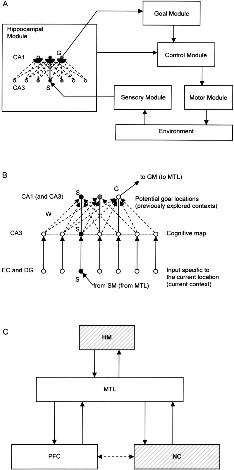
Architecture of the model. (A) General block-diagram of the model applied to spatial navigation. Arrows show input–output relations among the modules. Sensory module stimulates the CA3 unit S that represents the current location (or the currently perceived context) on the cognitive map. By assumption, the goal module can be “tuned” to a CA1 unit G that represents the location of the current goal. If, in addition, the goal module is modulated by the θ rhythm, it may be able to detect a moment of time of the strongest PP effect on G activity. In this case, the control module may be able to detect the momentary PP direction in CA3 that produces the strongest effects on G. For example, the control module may receive information from CA3 about spontaneous fluctuations of the PP direction. Based on this combined information about the momentary PP direction and the moment of G's strongest response to θ, the control module selects the next move and sends a command to motor module, which controls the motion of the model animal in its environment. The control module, the goal module, the sensory module, and the motor module were implemented algorithmically in the study of spatial and problem-solving paradigms. (B) Architecture of the hippocampal module. This module was implemented as a neural network with plastic excitatory connections. CA3-to-CA1 connection weights W were modified via the associative learning scheme (equation 1). Horizontal CA3-to-CA3 connections J, not present in spatial simulations, were essentially involved in simulations of all memory retrieval paradigms. S: Units representing the current location; G: units representing the goal location. Shades of gray represent unit activity. (C) Possible mapping of the model architecture onto brain structures. The hippocampal module maps onto the hippocampus proper in all cases. The control module maps onto the prefrontal cortex, PFC (e.g., dorsolateral PFC). When the model is applied to episodic memory-retrieval paradigms, the role of the environment is played by multimodal extrastriate sensory neocortices (the neocortical component, NC). Other components of the architecture A map onto MTL and/or PFC (cf. Fig. 5).

In the application of the model to spatial navigation, each small neighborhood in the environment has a unique representation in the system being associated with a particular CA3 unit and a particular CA1 unit. This is consistent with the (now widely accepted) view of rodent hippocampal pyramidal cells as place cells. Place cells have preferred locations in an environment characterized by a high firing rate of the cell. Any of these locations may happen to be a goal location under certain circumstances, and as such, we refer to them as “potential goals.” However, we do not assume that place cells specifically serve to represent goals.

We interpret the gradient of a firing-rate distribution of each place cell as encoded “driving directions” to the point of a maximal firing rate for this cell, which can be an arbitrarily selected point of the environment. In order to find a way to a goal, the system “listens” to the background activity of goal-related cells, while exploring alternative feasible actions during sequential θ cycles.

The model presupposes that, during exploration, the environment is navigated randomly, but extensively. However, as illustrated by Figure 3A, the system is not required to visit every location during exploration, and the frequency of visits (occupancy) during the exploration phase may not be evenly distributed among visited locations. Each visit to a particular location results in a strong activation of the corresponding CA3 and CA1 model units (Fig. 2). At various arbitrary moments during exploration, corresponding to the occurrence of sharp waves, the system pauses, and the current location is taken as a potential future goal. At this point, the activity mode changes from regular, θ-modulated place-cell firing to LIA with “sharp wave” reactivation of recently active CA3 place cells, with a firing rate proportional to the recency of their last strong activation. In addition, CA1 cells representing the current location are also reactivated (Buzsaki 1989). As a result, CA3 place cells become associated with the selected CA1 cell whose place field represents a potential future goal. The strength of the associations in this model is proportional to the recency of a place-cell firing during exploration:

1

where W_ij is the efficacy (weight) of the synaptic connection from CA3 unit j to CA1 unit i, t is the current moment of time, and t_j is the time stamp of the last visit to the location associated with the unit j during the running session. The initial conditions for W's are arbitrary small values below 1/L_max, where L_max is the maximal (allowed) trajectory length that can be associated with the goal during the training session. The weights of reciprocal connections are set to a constant (W_ii = 2). Generally, the exact functional dependence (equation 1) of W on t-t_j is not essential for the results of simulations, as long as the function remains strictly monotonic and noticeably decreasing with the distance.

Figure 3.

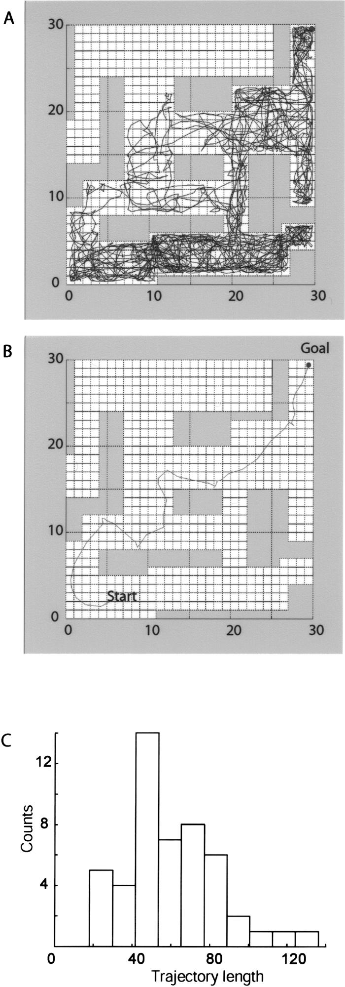
Simulation results for two-dimensional navigation. (A) A sample random trajectory during exploration of the maze. The CA1 unit subsequently selected as a goal represents the top, right corner square (black dot). Each square of the lattice corresponds to one CA3 unit of the model network that is a discrete graph; however, the simulated motion is continuous. The exploratory motion is controlled by equation 2 with randomly fluctuating acceleration a. The trajectory does not cover the maze uniformly; in fact, a large part of the maze remains unexplored (top, left area). The running starts at the bottom of the maze and is continued until the future goal location is reached. (B) A sample trajectory toward the goal following the learning session shown in A. In this case, the acceleration a in equation 2 is controlled by the model (Fig. 2) according to the algorithm described in the text. The trajectory in B is reasonably close by its length to a shortest path and is ∼60 times shorter than a typical random walk, e.g., the trajectory in A. (C) Histogram of goalsearch trajectory lengths for the learning scenario represented in A. The units of length correspond to those of A and B.

After the conclusion of an associative learning event, the system resumes random exploration of the environment, until another arbitrary potential goal is selected, and the associative process (a sharp wave) repeats. Thus, if the exploration phase continues until a preselected goal location is reached, the CA3 model units acquire potentiated, weighted connections to the CA1 representation of the goal. At this point, the network of place cells actually provides a capacity for finding a short path to this goal location, starting from any given location within the environment. This is accomplished by a simple algorithm; at each location, several randomly generated possible local moves are explored via PP, and the move that produces the strongest excitation of the place cell associated with the goal is selected and performed. This process is repeated until the goal is reached. In the case of two-dimensional spatial navigation, the PP direction fluctuates within a standard set (“right,” “left,” etc.) In the memory search paradigm (see below), PP explores those connections that are stored in the CA3-to-CA3 synaptic matrix. For the sake of parsimony, CA3-to-CA3 synapses are only included in the model of memory retrieval, and not in the model of spatial navigation.

Model architecture and its mapping onto the brain

In addition to the hippocampal module described above (Fig. 2B), the implementation of the spatial navigation algorithm implies the presence of an external “goal module” to interpret CA1 activity (Fig. 2A). The goal module is tuned to detect a maximal response during PP in the CA1 unit associated with the goal location. We assume that the goal module is also modulated by the θ frequency. In partial support of this assumption, is the observation that any “voluntary” movement of a rat, e.g., pressing of the “gas” pedal while driving a toy car, is phase-locked to the θ rhythm (Terrazas et al. 1997). The goal module is connected to a control module, which detects the PP direction that maximally excites the CA1 goal-related cell and selects the corresponding movement. A motor module connected to the control module executes this selection. A sensory module delivers the updated sensory and/or proprioceptive input translated into a new perceived context directly to the hippocampal module.

This model architecture can be mapped onto brain structures (Fig. 2C; see also Samsonovich and McNaughton 1997). Here, we emphasize one difference between the mapping of the model applied to spatial navigation and the mapping of the model applied to episodic memory retrieval. While the hippocampal module is mapped onto the hippocampus proper and plays the same functional role in both cases, the role of the environment (Fig. 2A) in a spatial navigation case is delegated to the extrastriate sensory neocortex (the neocortical component) (Fig. 2C) in the case of episodic memory retrieval. In particular, all episodic memory contents are assumed to be stored in this neocortical component. In the model applied to episodic memory retrieval, the control module maps onto PFC, while the functions of the goal, motor, and sensory modules are mediated by MTL and may also be partially attributed to PFC.

Computational implementation details

In order to apply the above general scheme (equation 1 and Fig. 2) to model a rat running in a typical experimental environment (e.g., Fig. 3A), a few more details need to be specified as follows: (1) the rat coordinates change continuously, (2) the animal possesses inertia, e.g., it cannot instantly stop or turn at a sharp angle, and (3) it is the acceleration rather than the location in space that the nervous system can control immediately. These features are captured by the following simplified equations of motion written in the discrete time t:

2

where x is the two-dimensional location of the rat, v is its velocity, and the Gaussian random variable a is its acceleration, which has a zero mean and a standard deviation σ. During initial exploration, any randomly generated value is accepted. During goal-directed search, the “voluntary control” is introduced algorithmically as the selection (by the control module) of one among several (10) randomly generated values of a with the strongest PP effect on the goal unit (therefore, not all possible values of a, which constitute a continuum, are explored). The motion is dissipative; the model rat velocity decays over time with the exponent log α. The CA3 and CA1 units to be activated are selected at each discrete time step via rounding of x toward the nearest integer vector.

The values of parameters used in the simulations of Figure 3 were α = 0.875, σ² = 0.5. In addition, v was reset to zero at each bump into a wall. The numerical values of α and σ determine the average speed of motion and were adjusted to yield realistic rat-like trajectories. Primarily, however, the realism of the trajectories achieved by the model is due to the choice of equations of motion (equation 2) that describe the control of acceleration rather than position. Within the range of values for the parameters of equation 2 that provided realistic trajectories, the qualitative simulation results were robust and not sensitive to particular parameter combinations.

Nonspatial paradigms

In the case of the space of states of the three-disc Tower of Hanoi problem, only discrete transitions between neighboring nodes of the graph (Fig. 4A) constitute possible movements. Therefore, equations of motion (equation 2) were not used in this case. Instead, 10 randomly generated (possibly repeating) moves were probed at each node before selecting the best of them based on the associated weights, as described above. All other implementation details were the same as in the previous case.

Figure 4.

Tower of Hanoi Paradigm. (A) The discrete space of states of the classic Tower of Hanoi Puzzle with three discs. Gray triangles represent states of the puzzle that are depicted next to them. Lines connecting triangles show all possible moves (small disk, solid line; middle disk, dashed line; large disk, dotted line). (B) The time used by the system to solve the Tower of Hanoi puzzle vs. the time allowed for random exploration of the puzzle before disclosing the goal. A unit of time is one move. Each box represents results of 10 independent trials (all with random starting configuration) and has lines at the lower quartile, median, and upper quartile values. Whiskers represent the rest of the data range. A sharp transition can be seen at ∼100 exploratory moves.

To simulate an example of episodic memory retrieval event (Fig. 5), we use essentially the same model architecture (Fig. 2A) and dynamical rules as in the previous case, implementing only the following modifications. CA3 layer in the hippocampal module has now internal synapses (Fig. 2B; horizontal links), which store connections of the cognitive graph. Environment is replaced with a separate neural network representing the neocortical component. The implementational details of this component are described in the next subsection. The stable patterns in this neocortical network are attractors taken to represent “episodic memories.” Each of these patterns is assumed to be previously explored and associated with the hippocampal module units, thus binding together the dynamics of the two components. During the random memory exploration phase, the weights W are adjusted according to equation 1, and local CA3- to-CA3 connections are created corresponding to the transitions among attractors in the neocortical component. The memory-search phase proceeds exactly as the goal-search phase in the Hanoi Tower simulations, except that, now, two neural networks, hippocampal and neocortical, are working in parallel.

Figure 5.

Modeling an example case of episodic memory retrieval. According to the proposed model, if the target episode (E) happened under unusual circumstances, then reactivating its hippocampal pointer immediately may not result in retrieval. Instead, the system must retrieve the key episodes (B, D) first in order to make the necessary contextual information available for the working memory. In the represented example, this is achieved by sequential activation of the pointers A, B, D, and E in the hippocampal module (HM) (cf. Fig. 2), as described in the text. (PFC) Prefrontal cortex performing the control and monitoring functions during strategic search; (MTL) medial temporal lobe cortices, the semantic memory storage; (NC) extrastriate sensory neocortex, where the memory content is presumably stored. The chain of thin black arrows outside of the hippocampal module shows the sequence of original experiences. Fat gray arrows inside of the hippocampal module show the path of retrieval. Other fat gray arrows show critical interactions among modules at the beginning of retrieval. Dotted arrows show hippocampal-to-neocortical associations (that are actually mediated by MTL; this detail is not shown). Thin black arrows inside of the hippocampal module show potential connections between A, B, C, D, and E. As explained in the text, these connections reflect logical and informational interdependence of remembered episodes (e.g., power outage in NIH makes sense in the context of a strong hurricane). Accordingly, these thin solid arrows agree one-to-one with all possible transitions in the simulated model the neocortical component (Fig. 6).

Attractor model of the neocortical component

A simple model of the neocortical component was simulated explicitly to illustrate the role of the hippocampus in an example of memory retrieval (Figs. 5, 6, 7). The neocortical component was implemented as an attractor network of neuronal units characterized by their activity rates v_i (equation 3):

3

Here, r_i are abstract, randomly generated two-dimensional coordinates assigned to each model unit (Fig. 6), I is the strength of the external input to the network from a hippocampal pointer (via MTL), the parameter σ_o and the “location” determine the input pattern. The state of the neocortical component at any moment of time is regarded as nearly stationary (i.e., variables v_i are considered fast) at the scale of the hippocampal module dynamics. The (asymmetric) synaptic weights w are randomly generated according to the formula

4

where ω_ij are independent random numbers uniformly distributed in the interval (0,1), ν is a constant inhibitory parameter (which stabilizes connectivity), and S is a standard logistic sigmoid function:

5

The firing rate in equation 3 was solved iteratively with values of model parameters n = 300, I = 3, σ = 0.15, σ_o = 0.2, ν =0.1, θ = 3. Given a specific realization of random numbers (produced by Matlab code included in Supplemental online material at http://www.krasnow.gmu.edu/ascoli/sa_lm05_som/), this network has six attractor states. Five of these are characterized by focused activity patterns represented in Figure 5, A–E. The sixth state has a near-zero, almost uniform distribution of activity (v = 0.032 + 0.005) and it can only be reached after a “cold” start.

Figure 6.

Simulation results for the model neocortical network. (A–E) Five stationary attractor states of the model neocortical component defined by equations 3 and 4, and by the realization of random numbers (see Materials and Methods and Supplemental online material at http://www.krasnow.gmu.edu/ascoli/sa_lm05_som/). Shades of gray represent unit activity. The “centers of mass” of activity in these five states are labeled a, b, c, d, and e, respectively. (A1) The network initially brought to the attractor state A is stimulated by the “pointer” E (a Gaussian distribution of inputs centered at the label “e”). The represented configuration is stationary under given conditions; the stimulus-induced transition from state A to state E does not occur. All possible stimulus-induced transitions in this model network are shown by thin black arrows inside of the hippocampal module circle in Figure 5. The reader can verify this fact, using the demo included in Supplemental online material at (http://www.krasnow.gmu.edu/ascoli/sa_lm05_som/).

Figure 7.

Architecture of the hippocampal module after the exploration phase in the example of episodic memory retrieval. These numerical results of learning in the hippocampal module were achieved in a typical memory-exploring sequence of 10 moves (Supplemental online material at http://www.krasnow.gmu.edu/ascoli/sa_lm05_som/: the movie “exploration”). Labels A–E within the circles correspond to the hippocampal pointers in Figure 5 and the related stable neocortical patterns in Figure 6. Solid CA3-to-CA3 arrows (bottom) show explored (and stored in the hippocampal module) transitions among memories in the neocortical component. Dashed CA3-to-CA3 arrows show available, yet unexplored transitions. Despite the unexplored part of connections, all-to-all off-diagonal synaptic weights W (vertical oblique arrows of variable thickness) were modified by learning according to equation 1 in this simulation. The thickness of each arrow is proportional to the corresponding computed synaptic weight W, which varies from 0.2 to 1.0. Straight vertical CA3-to-CA1 dotted lines that represent diagonal matrix elements had the maximal weight W_ii = 2.

The implementation of this model corresponds to a fairly standard artificial neural network, with Gaussian input and Gaussian distribution of synaptic weights. The goal of this neocortical component simulation is not to embody a biologically plausible representation of the neocortex, nor to offer a mechanistic insight into its function. Instead, this model is one of the simplest network implementations yielding nontrivial dynamics among stable activity patterns. We take the transitions among these activity patterns to illustrate sequential episodes in the space of memories. Thus, this neocortical network was only used to analyze the role of the hippocampal module in a simple memory retrieval paradigm. Other network models with dynamical activity patterns that could represent episodic memories could serve the same purpose.

Simulation of the hippocampal module as a large two-layer neural network

In order to address the biological plausibility of the hippocampal model for episodic memory retrieval under realistic conditions (e.g., in terms of the size of memory space, number of visited episodes during memory exploration, number of episodes necessary to reach an arbitrary target during retrieval, etc.), we implemented a larger scale hippocampal module model. The network was composed of N CA3 plus N CA1 model neuronal units (N = 11, 20, 30, 50, 100, 200, 300, 500, 1000, 2000, 3000, 5000, 10,000, 20,000, 30,000). Each unit was considered as a group of principal hippocampal cells representing a unique, previously explored abstract context, with one-to-one correspondence between CA3 and CA1 units. Selected random connections between abstract contexts were stored in the CA3-to-CA3 synapses (matrix J). Each CA3 unit was associated with 10 other randomly selected CA3 units (with the uniform probability, but avoiding repetitions). An interpretation of these stored connections is that they result from associative learning during initial experience and during subsequent off-line replays. One epoch of memory exploration was simulated for each afferent connection of each CA3 unit. Each epoch included M steps connecting M + 1 units (M ranging from 1 to 100 in different simulations). Technically, these exploratory epochs were simulated by sequentially activating the stored connections J backward. All CA3 units that were active during a given epoch were associated with the CA1 unit that was active at the end of the epoch, with the weight given by equation 1, where t_j is the time of the last reactivation of unit j during the epoch. Associations across different epochs were not created.

During retrieval, the activity in CA3 was centered on one unit and distributed with the weight 0.2 among all 10 efferent neighbors of the central unit. The resultant profile of the CA3 activity packet is represented in Figure 8A. The corresponding distribution of activity in CA1 (Fig. 8B) was calculated as the distribution of activity in CA3 multiplied by the matrix W. When stated explicitly, a Gaussian, uncorrelated noise was added to the resulting CA1 activity. The standard deviation of noise ranged from 0 to 0.0015, i.e., 2.5% of the peak CA1 activity value (this level of noise is attributed to individual model units, each of which may be related to a large population of neurons). In addition, both CA3 and CA1 activity packets performed PP oscillations in synchrony with each other. The direction of PP was alternated, so that all 10 stored efferent connections were explored at each visited location. As before, a PP oscillation that produced the strongest effect on the goal-related CA1 cell was selected as the next step. If there was no effect, a random efferent connection of the current CA3 unit was selected as the next step. The process of retrieval was terminated when the goal-related CA1 cell became the center of the CA1 activity packet. In each retrieval simulation session, both the starting and the target units were randomly selected anew. The Matlab code used in all simulations is included in Supplemental online material at http://www.krasnow.gmu.edu/ascoli/sa_lm05_som/.

Figure 8.

Simulation results for the random hippocampal network. (A) Shape of CA3 activity packet in the model. (B) Activity packet shape in CA1 analytically calculated from the CA3 shape (A) in the limit of a large number of units N. The distance from the center is measured along stored efferent connections. The distribution is truncated at the distance M = 5. The uniform background activity level, which did not affect any model dynamics, was set to zero. The sum of activity over the layer is normalized to 1. The central peak value is 0.06; the standard deviation of the distribution is 1.0. (C) Histogram of retrieval trajectory lengths calculated over 10,000 retrieval sessions with a randomly generated network of 10,000 units. The plot represents 99.6% of all trajectories (see text). (D) Dependence of the retrieval path length on the number of episodes in each sequence (epoch) used in associative learning and on the level of noise. Epochs of spontaneous, random, off-line replay of memory episodes (propagating along stored connections) were simulated to create associations between CA3 and CA1 units (matrix W) according to equation 1. One trajectory per afferent connection was associated with each unit (totalling, on average, 10 trajectories per unit, each of the length M). In subsequent retrieval sessions (10⁴ sessions per data point), the average length of a retrieval path was a decreasing function of the number of episodes in the sequences, as the plot shows. (Solid lines) No noise added to CA1 unit activity; (dashed lines) a white Gaussian noise (2.5% of the peak CA1 activity) was added to all active CA1 units. Middle lines represent the mean value; bars show the standard deviation. The three dotted horizontal straight lines show the mean plus-minus of the standard deviation of the shortest path lengths in 10⁴ runs. (E) Dependence of the retrieval path length (solid lines) on the memory load (the number of units) N. The triplet of dotted straight lines shows the dependence of the shortest path length on N (computed with the same data set, the mean ± the standard deviation). The vertical dotted line shows the approximate real number of recurrent synapses per pyramidal cell in CA3, which may determine the upper limit on the episodic memory load, i.e., the number of patterns stored in CA3 (in the model, this limit is given by the number N of model CA3 units).

Results

Simulated navigation in a continuous two-dimensional space

We start by describing simulation results for a two-dimensional maze shown in Figure 3. After random exploration of the environment (that starts at the bottom and ends in the upper right corner; Fig. 3A), the model rat is given the task to reach a preselected goal. The typical resulting trajectory steers clear of dead ends and does not includes loops (Fig. 3B). Most importantly, when starting from any of the previously explored locations, the model reaches the goal following a path with length of the same order of that of the shortest possible path.

Figure 3C shows a histogram of 50 trajectory lengths for the learning session represented in Figure 3A, when the starting location is selected at random for each trajectory, and the goal location is fixed. The long tail on the right side is due to the selection of starting locations within the unexplored area (the upper left part in Fig. 3A). In this case, the model rat proceeds randomly until it reaches a previously explored location. The average ratio of the length of the trajectory leading to the goal before and after learning was 60:1.

Simulated solution of the Tower of Hanoi problem

The qualitative results obtained with this model in simulated mazes are not contingent on the geometrical and topological properties of the search space (such as continuity and planarity of the environment, symmetry of connections, etc.) and can be reproduced in nonspatial problem solving. The classic Tower of Hanoi puzzle (analyzed, e.g., in Russell and Norvig 1995) is an example of a nonspatial problem that can be solved by the same algorithm used above for two-dimensional navigation. Figure 4A represents the entire space of states of the three-disc Tower of Hanoi problem.

One hundred independent sessions of the exploration-and-solving paradigm were run. The system had no a priori knowledge of the goal during the exploration phase, in which associations were learned according to equation 1. The exploration time was doubled every 10 cycles. During each of the exploratory epochs (all started with a randomly generated configuration) the goal could be reached 0, 1, or several times. The resulting distribution of the solving time vs. exploration time is presented in Figure 4B. Instead of a gradual decrease in the average solving time, a sharp transition is observed at ∼100 exploratory moves, when the probability that the goal is not reached during the exploration phase becomes negligible. The system always (and immediately) finds a nearly optimal path in the discrete search space, provided that every location is previously explored.

Episodic retrieval involving navigation of memory

Here, we present a simple model description of a realistic example of episodic memory retrieval. A critical element of this example is that the episode to be retrieved requires other episodic knowledge for its understanding. This case is crucially distinct from retrieval of typical episodes. In the retrieval of a typical episode (“What did you have for breakfast last Monday?”), PFC can be used to immediately access facts from semantic memory in MTL that are highly accessible insofar as they have been stamped in by multiple experiences as follows: “What do I normally do on Mondays? I go to the National Institute of Health (NIH). What do I normally have for breakfast? Orange juice. Where do I normally eat breakfast? At a cafeteria.” As a result of this process, the system may produce a rather trivial answer; “I had an orange juice at the NIH cafeteria.” This account, however, may not apply to memories of unique, unusual episodes. Imagine that the above answers are not characteristic of you at all. You do not go to NIH regularly. You eat breakfast at home, and you never drink orange juice in the morning. Yet someone tells you the following: “I saw you last Monday morning at the NIH cafeteria with orange juice!” In order to be able to retrieve and to understand a memory of this episode (assuming that it did take place), you may need to retrieve several related episodes first that contain key episodic (rather than semantic) memory data. Those related key episodes may be involved with completely different semantic features, and in this case, PFC may not be able to find them without the help of the hippocampus (Fig. 5). Our model allows for the following account of this case.

1. At the beginning, PFC tunes to receiving signals from MTL related to specific semantic features of the target episode, namely, “orange juice,”“NIH cafeteria,” and the notion of last Monday. Suppose that pointer E (Fig. 5) is the only perfect match for these features, and it is associated with the right memory. Nevertheless, activating this pointer immediately may not help in retrieval of the episode.

2. Next, PFC attempts to activate any semantic features (schemas) associated with connections from the current context (at the beginning, this is the context of talking to a friend) to other contexts, while “listening” to the background activity in E via the two selected features. Suppose that the strongest response in E at the first step of retrieval is associated with simultaneous activation of two schemas, “morning hurricanes” and “seminars at NIH” (Fig. 5).

3. Therefore, the system activates these features in MTL, thereby causing a transition along the connection from A to B in the hippocampal module. The corresponding alteration of the activity pattern in the neocortical component is induced (Fig. 6); as the pointer B becomes active, the episode B is retrieved in the neocortical component, corresponding to the arrival to NIH for a morning seminar, when a strong hurricane is beginning.

4. The pattern of action (2 and 3) is repeated (e.g., the next retrieved key episode would be the moment of power and water outage at NIH), until the system reaches the target pointer E in the hippocampal module and the associated target episode E in the neocortical component. This is the moment of ordering orange juice at the NIH cafeteria, because no other drink is available. The resultant path (fat gray lines inside the hippocampal module, Fig. 5) is shorter than the original sequence of experience (the chain of thin black arrows outside of the hippocampal module, Fig. 5).

In order to illustrate the possible role of the hippocampus in the above process, we apply another instance of the the hippocampal module network (Fig. 2) to this problem. The role of the environment in this case is played by the attractor network model of the neocortical component. In this model, neuronal units are randomly allocated on a plane, with potentially all-to-all connections limited by a Gaussian function of the distance (see Materials and Methods section above). In the particular realization of the network we used, five attractor states are compact patterns of activity (Fig. 6), which can be taken to correspond to episodes A–E in Figure 5. The model neocortical network was simulated in parallel with the original hippocampus model (Fig. 2B), described by equation 1, and taken in the form of the graph represented in Figure 5 (hippocampal module). The output from an active hippocampal module unit was distributed among inputs of the neocortical component units using a Gaussian function centered at a location (a, b, c, d, or e) associated with the the hippocampal module unit. During an interval between stimulations, the neocortical component relaxed to an attractor state. Thus, possible control actions over the neocortical component were limited to activation of one (or none) of the “pointers” that project to neighborhoods a, b, c, d, and e in Figure 6, while the role of the hippocampal module and related structures (Fig. 2) was to find the right sequence of activation of the neocortical component.

The neocortical network's dynamics were not governed by geometrical distances between attractor centers. Transitions between well-separated, distant patterns (e.g., from E to C) were readily induced by the stimulus. At the same time, some transitions between nearby overlapping patterns did not occur. For example, when the network was in state A, and the stimulus was applied at the label e, attractor state A was slightly distorted (Fig. 6A1), but it did not jump to the pattern E. All connections in the model network (i.e., transitions that can be caused by a stimulus applied at a, b, c, d, or e) are represented by thin black arrows connecting pointers A–E inside of the hippocampal component in Figure 5. In particular, the network can be led to E from A via B and D, but not directly from A to E. This result illustrates the idea that in some neuronal networks, contrary to the traditional theory going back to Teyler and Discenna (1985, 1986), a premature reactivation of a hippocampal pointer associated with the target episode may not cause retrieval of the episodic memory, while at the same time reactivation of a connected path successfully results in retrieval.

During one selected typical training session in simulations of this example (captured in the movie “exploration” included in Supplemental online material at http://www.krasnow.gmu.edu/ascoli/sa_lm05_som/), the system randomly explored possible transitions between pointers in the hippocampal module. The system followed (and stored in CA3-to-CA3 synapses J) only those transitions that successfully induced the correspondent pattern switching in the neocortical component. In parallel, the matrix W was modified according to equation 1. This memory exploration phase lasted for 10 steps. The resultant matrices J and W are represented in Figure 7 by the thickness and the style of lines (see Fig. 7 caption). The reader can easily reconstruct the path from A to E that was selected by the model in the retrieval phase, when the pointer E was given as a goal (see the movie “retrieval” included in Supplemental online material at http://www.krasnow.gmu.edu/ascoli/sa_lm05_som/). To reconstruct the path, the reader may follow at each step a solid CA3-to-CA3 arrow leading to a CA3 node with the strongest connection to CA1 node E (this path is A → B → D → E).

The function of this rather simple example simulation is to illustrate the possible involvement of the hippocampal network in the retrieval of an unusual episodic memory, as in the example presented in Figure 5. In particular, the attractor network model of the neocortical component allows the implementation of episodic memory dynamics in parallel with the hippocampal network. The particular choice of the neocortical component model does not affect the plausibility of the hippocampal module. Nevertheless, several critical questions remain open regarding the applicability of the hippocampal network model in conditions closer to real episodic memory retrieval. How does the model perform in the case of a large, realistic memory load? How many sequential episodes in this case should be associated with a CA1 unit in a sharp wave for the model to succeed in retrieval? Can the model remain efficient, if more realistically spread distributions of activity are used in CA3 and in CA1 instead of a single winner-take-all unit? Finally, how robust is the model performance with respect to the intrinsic noise that is due to the random and discrete nature of neuronal spikes?

Episodic memory retrieval with a substantially large memory load

In order to address the above questions, we increased the size of the hippocampal module network up to 30,000 units representing abstract contexts. To the best of our knowledge, the number of distinct contexts remembered by a typical, normal adult human has not yet been reliably estimated. At the same time, assuming that the pointers to those contexts are stored in the hippocampus, one may come up with an estimate based on the anatomical data (see Connectivity in Cornu Ammonis). CA3 network is frequently considered as an autoassociative attractor network. In many theoretical models of autoassociative attractor neural networks (Amit 1989; Hertz et al. 1991) the decimal order of the maximal number of stored patterns can be roughly estimated as the decimal order of the number of synapses per neuron. Based on this logic, we take the number 10⁴ as a “realistic” estimate of a typical episodic memory load. While this number intuitively appears low, most long-term memories may be of semantic nature, and therefore, their retrieval may not primarily depend on the hippocampus.

In this simulation, we implemented the hippocampal module as a large, randomly generated two-layer network with the total number of neuronal units up to 6 × 10⁴ and the total number of modified synapses up to 3 × 10⁶ (the corresponding maximal total number of synapses was of the order of 10⁹). The neocortical component was not explicitly simulated in this case. Instead, random connections were generated (and stored in J) during training sessions. We used a more realistic model activity distribution in CA3 (Fig. 8A), which resulted in a more realistic activity packet shape in CA1 (Fig. 8B). For each randomly generated and explored network, 10⁴ retrieval sessions were run, with a random selection of both the starting and the goal locations in each session. Among the varied parameters of the model were the number of episodes (or abstract concepts) associated with CA1 units in sharp waves, and the level of dynamical noise in CA1. Results are presented in Figure 8. The main finding is the robust ability of this model system to find a nearly optimal path toward a given target.

For example, consider the memory load N = 10⁴, with n = 10 efferent connections per hippocampal module unit, with M = 5 exploration steps of sequential episodes to be associated with a CA1 unit, in the absence of noise. In these realistic conditions, the retrieval path length between two randomly selected units (calculated over 10⁴ retrieval sessions, each with random start and goal selection) is 6.75 ± 3.10sd, while the shortest path length (calculated in parallel for the same set of cases) is 4.22 ± 0.68. The ratio of the mean values is 1.6, and the second interval is almost entirely contained within the first. The histogram of retrieval path lengths at these values of parameters is compact (Fig. 8C), with all of the 10⁴ trajectories shorter than 60 steps, and 99.5% of them shorter than 20 steps. To compare, a typical random trajectory connecting two randomly selected units in this model network consists of the order of 7000 steps. This estimate also holds for the case when the two selected units coincide, meaning that a random traveler in this huge space would be lost practically forever after the very first step. Nevertheless, our hippocampal network model was never lost.

This result is robust with respect to alteration of many model parameters within and beyond their realistic range (Fig. 8). For example, introducing Gaussian dynamic noise at the level of 2.5% of the peak CA1 activity only increases the mean retrieval path length by 9%. Doubling the number of units N increases the mean retrieval path length by 30% (while at the same time, the mean shortest path length increases by 7%). Shortening the number of associated episodes M from five to two increases the mean retrieval path length by 11% (Fig. 7D). Therefore, unlike the case of spatial navigation of large two-dimensional environments, this paradigm of memory retrieval does not require long exploration epochs to be associated with potential target units. On the contrary, association of very short epochs may suffice for a reasonably good performance. At the same time, increasing M up to 100 and beyond does not significantly improve the performance of the model.

Discussion

The last simulation constitutes a proof-by-example of the viability of the proposed concept in the case of an abstract model system with a realistically large memory load. Can the same phenomenon be demonstrated in a network with more realistic architecture and dynamics? One way to improve the model is by using a more precise description of the distribution of activity in CA3 and in CA1. For example, extending the rapidly descending tails of the activity packet in CA3 (Fig. 7B) up to the next-to-nearest neighbors of the central unit should improve the performance of the system, in particular, in the case of a very large network (10⁵ units and above). This idea is consistent with the broad spatial tuning of place cells in CA3 (in addition to CA1). Another interesting possible modification of the model concerns the architecture of the random network. Here, we assumed that the probability of connection is uniformly distributed among units (with the only constraint that there are 10 efferent connections for each unit). Instead, a subset of units that are connected to the same parent could have a higher probability to be connected to each other than to any randomly selected unit. This bias, if present, would result in a certain degree of clustering in the network, consistent with the idea of cell assemblies (Harris et al. 2003), as well as with the hierarchical organization of remembered contexts.

Understanding hippocampal function in episodic memory retrieval

According to the view of the hippocampus as a context-indexing device (e.g., Wheeler et al. 1997), all real or imagined general contexts of experiences (rather than experiences per se) are represented by distinct hippocampal activity states. Neural activity in each of these states is focused on a relatively small, uniquely selected subpopulation of principal cells. Each state of this sort could possess certain (meta-) stability typical of a latent attractor state (Samsonovich and McNaughton 1997; Doboli et al. 2000). The most commonly held account of the neural basis of contextual reinstatement is that PFC is used to access information in semantic memory (Shimamura 1995; Moscovitch 1992; Dobbins et al. 2002) that is stored in MTL, and not in the hippocampus (Vargha-Khadem et al. 1997) nor in PFC (e.g., Sylvester and Shimamura 2002). PFC then maintains this information in working memory and uses it to cue the hippocampus. The goal of the contextual reinstatement process would be to provide enough details that match the hippocampal memory trace, so that it is triggered. Specific information retrieved from the hippocampus can be used to further refine the retrieval cue (e.g., Howard and Kahana 2002). Finally, according to this view, when the correct hippocampal pointer is reactivated, the entire episodic memory content, distributed across modalities in the neocortical component, is retrieved. This traditional view makes two essential (if implicit) assumptions, that we choose to drop.

1. All contextual information necessary for understanding an episode is associated with the memory trace of experience (possibly, via the hippocampal pointer).

2. Once the hippocampal pointer associated with an episodic memory trace is activated, the entire trace is automatically reactivated.

Departing from these assumptions, the present work hypothesized that the goal of gradual contextual reinstatement is not to find the hippocampal pointer (which might be known to PFC even at the beginning of the process), but to prepare the neocortical component for the retrieval of the target memory trace. This is done by reinstating into the neocortical component, step by step, the necessary contextual information that is missing in its memory traces. In our model, this goal is achieved by “driving” the neocortical component through a sequence of its dynamical states. In other words, the necessary context is made available by a recent history of activity of the system, i.e., by a path in the memory space. This path must be found every time the memory is accessed, and it must consist of available connections only. Thus, the proposed model can be roughly summarized as the following: The key for episodic retrieval is the missing context, the key for this context reconstruction is a path in memory space found by the hippocampus, and the key for pathfinding is the mechanism involving exploration of available connections while “listening” to a goal-related cell. This picture can be considered complementary rather than alternative to the traditional view of the hippocampus as a memory index, or a cognitive map, or a multimodal associator.

Six testable predictions of the theory

(1) A testable prediction of our model in the domain of episodic memory studies is that hippocampal or prefrontal damage may severely impair the ability to recall by a cue those episodes that require other unique episodic knowledge for their understanding. Present experimental data demonstrate that frontal lesions result in impairment of strategic recall, not cued recall of “episodic memories” in paired-word list learning paradigms. Moreover, when a recall strategy is supplied, frontal lesion subjects perform as well as normal controls (Dellarocchetta and Milner 1993). To the best of our knowledge, the differential quality of cued recall of unique and unusual vs. typical episodes in hippocampal or prefrontal lesion cases was not assessed experimentally. Our prediction is consistent with other available experimental data (e.g., Westmacot et al. 2001).

(2) Another prediction of our model in the domain of episodic memory studies relates to scopolamine-induced (Potter et al. 2000) or stress-induced (Yovell et al. 2003) hippocampal amnesia. We consider a conceivable case, when episodic memory failure may result from disconnection of a cluster of hippocampal pointers from the rest of the cognitive graph, rather than from the absence of these pointers. Obliteration of a key episode associated with essential contextual information may render all subsequent cluster of events inaccessible by free or cued recall. In this case, our model predicts that each episode of the cluster may still be recognizable given enough details, and that successful retrieval of any of these episodes should make the rest of the cluster immediately available for free recall.

(3) Spatial navigation was used here as a “proving ground” to illustrate the more general model of memory retrieval. The proposed model of spatial navigation is based on a novel assumption about the semantics of place-cell firing, namely, that the gradient of the firing rate distribution encodes “common sense directions,” i.e., it points to the first step along a reasonably short path leading to the place field center, rather than the direction of the radius vector to that location. Thus, a nontrivial prediction of the model regarding the place-cell phenomenon is that the firing rate distribution should be more strongly correlated with the shortest explored path distance than with the Euclidean distance to the center of the place field. In particular, we expect place fields to be discontinuous at a thin barrier partitioning the environment, as seen in results of previous studies with a simpler version of this model (Samsonovich and Ascoli 2001). This prediction diverges from the hypothesis of a prewired, continuous two-dimensional map with near-Euclidean metrics (McNaughton et al. 1996), which is supported by the data of Wilson and McNaughton (1993). Other available experimental observations favor our view. For example, Skaggs and McNaughton (1998) found significant discontinuity of place fields at a very thin partition separating two identical boxes, regardless of whether the hippocampal representations of these two boxes were very similar or very different from each other (see also Lever et al. 1999, and the discussion of their result in Hartley et al. 2000). These observations, however, could also be interpreted in terms of two different hippocampal maps (Samsonovich and McNaughton 1997) associated with the two sides of the barrier. Therefore, a more conclusive test is desirable, including an assessment of “remapping” (typically detected as a simultaneous, substantial alteration of all place-cell firing rates). For those cases when remapping can be excluded, we predict that one can nevertheless observe a strong discontinuity in one or more place-cell firing rate distributions across a thin barrier.

(4) Place-cell firing in our model is not sensitive to the direction of motion or the orientation of the head, as well as the past and future trajectory parts, and depends on the current animal's location only. The experimentally observed directionality of place fields on linear tracks (Gothard et al. 1996) and the so-called phenomena of “prospective” and “retrospective” coding (Ferbinteanu and Shapiro 2003; Battaglia et al. 2004) may have different origin, again related to “remapping.” Usually, in the case of one-dimensional motion, the hippocampus develops separate maps for each direction (Gothard et al. 1996) and typically for each behavioral paradigm as well (e.g., Markus et al. 1995); however, some cells show activity on two maps with identical or close positions of the place-field maxima. Our model predicts that these place fields will develop tails in opposite directions and eventually become adjacent to each other, with a small overlap (tiling). According to our model, the point of overlap, which is also initially the point of maximal firing rate of the cell on both maps, is likely to be a place where the rat stops. All of these features can be actually observed in the data of Markus et al. (1995), their Figure 10, G and H, and Battaglia et al. (2004); however, more observations are necessary for a definitive conclusion.

(5) Also supporting the above predictions are observations of the skewness of rodent hippocampal place fields on a linear track that gradually develops over time, if the animal runs in one direction only (Mehta et al. 2000). In our model, the shape of CA3 place fields during circular one-dimensional motion at constant speed is qualitatively given by equation 1, where W roughly represents the amplitude of the background place-cell activity (the main peak is assumed to be well focused), and t-t_j can be replaced by an angle (ranging from 0 to 360° in the direction opposite to the direction of motion) from the location of the selected CA1 place-cell peak activity. Since all laps are identical (the speed is assumed constant), the first argument of the max in equation 1 may be ignored, and the place-cell distribution can be visualized as having a sharp peak at the maximum of the CA1 place-cell firing, and a long tail that extends to one side only (cf. Mehta et al. 1997). Moreover, the related phenomenon of place-field smearing (Mehta et al. 1997, 2000) also naturally results from the model learning rules (equation 1). In the above example of multiple laps around a circle, if the speed is random instead of constant, the amplitude W at each location distant from the place-field maximum should be calculated based on the best timing among all laps, according to equation 1. Therefore, W will generally increase with time upon continual motion, as reported by Mehta et al. (1997, 2000).

(6) The fine structure of the fan-out PP pattern (Fig. 1F) assumed by our model could be observed experimentally, and leads to specific quantitative predictions. Each spike of a place cell can be characterized by a 2-D unit vector in the current egocentric coordinates of the rat, pointing toward the place-field maximum of the spiking cell. According to the model, the hippocampus spontaneously “explores” alternative directions of motion in sequential θ cycles. If this is the case, egocentric direction vectors of two spiking cells should be more strongly correlated when the two spikes belong to the same θ cycle than when they belong to different (e.g., consecutive) θ cycles. Moreover, the pattern (Fig. 1F) suggests that the effect should be stronger for two spikes occurring at late (rather than early) θ phases.

Related works

The unifying theory of hippocampal memory and spatial function presented here is consistent with currently available experimental data on rodent place cells and human episodic memory. Although the two experimental domains are species separated, recent studies indicate consistency of general results across species (Ekstrom et al. 2003; Eacott and Norman 2004). In spite of many general discussions of conceptual unification of the hippocampal spatial and mnemonic functions (e.g., McNaughton et al. 1996; Redish and Touretzky 1997; Wallenstein et al. 1998), few proposals were specific at the level of underlying mechanisms. Burgess (2002) supposes that retrieval of spatial information from long-term storage requires the imposition of a particular viewpoint. The model is supported by hemispatial neglect data. Related ideas were described in a human case study by Luria (1968). In contrast with a local-view approach, an idea that the hippocampus is involved in movement control is central in the unification attempt by Gaffan (1998). Another proposal is the concept of attractor-map-based internal cognitive model (Samsonovich and McNaughton 1997). The present work introduces the first computational model describing plausible mechanisms of memory retrieval by navigation in an abstract cognitive space, showing that the same mechanisms can work in the case of ordinary spatial navigation. Many aspects of our ideas have been discussed and reviewed in previous works (e.g., Redish 1999; Eichenbaum 2004), but never integrated and directly implemented in a computational model. A number of previous models account for the hippocampal role in spatial navigation only, some of which have elements of similarity with the present work.

Gerstner and Abbott (1997) proposed a model of hippocampal map formation based on temporally asymmetric associative learning, in which place cell activity may be entrained to indicate the direction to a fixed target from any location, avoiding walls and other obstacles. In their model, however, directions to different goals can only be stored on different hippocampal maps. In contrast, in the available experimental literature, typically only one or (more rarely) two hippocampal maps are reported for an individual rat in a given environment. Therefore, based on the model of Gerstner and Abbott, rats should not be able to find an optimal path toward arbitrary locations in a familiar environment.

Trullier and Meyer (2000) introduced a network that learns temporal sequences of visited places, and exploits the resulting topological representation of the environment for navigation and path retrieval. Similar to the model described in the present study, this network learns to find paths during exploration without the need of any reinforcement. Trullier and Meyer's model learns the topology of the environment and sequences of moves, calling upon head-direction cells and a series of goal and subgoal cells to navigate the environment. However, it does not use individual CA1 place fields for directly encoding directional instructions to reach the center of the field. In contrast with theirs, our model of spatial navigation does not depend on stored sequences of moves, nor topological connections between neighboring locations, yet it is similarly capable of finding an optimal sequence of moves to reach an arbitrary target given a posteriori.

In the study of spatial navigation, we used learning mechanisms corresponding to the long-term potentiation (LTP) of CA3-to-CA1 excitatory synapses only. In the model of episodic memory retrieval, however, we took into account the formation of autoassociations within CA3 based on LTP in recurrent connections between recently active CA3 units. Indeed, many events in CA3-to-CA3 connections during sharp waves are analogous to those in CA3-to-CA1 connections. The introduction of this detail into the model appears to be necessary for efficient retrieval in a large network (Fig. 8). It is interesting to speculate how vital (if helpful) these effects might be for spatial learning and navigation. Recent studies (Nakazawa et al. 2003) show that N-methyl-D-aspartate (NMDA) receptors (traditionally implicated in associative LTP) in CA3 are necessary for normal place-field development and spatial learning in adult rat. These possibilities could be explored with the second version of our model applied to spatial navigation. Similar choice is made in several related models, including that of Trullier and Meyer (2000) discussed above, and models developed by Schmajuk and colleagues (e.g, Schmajuk and Thieme 1992; Voicu and Schmajuk 2001). Important differences between these works and the model presented here are the assumed (or predicted) firing properties of CA3 and CA1 place cells. In the above models, activity in CA3 during the θ mode propagates on a currently active map, dubiously covering up to half or more of the environment, to include the goal location. In contrast, and in closer agreement with the experimental data, in our model, the activity packet is always centered at the current location of the rat and covers a small fraction of the entire available area, a fraction that remains stable over time for as long as the rat is running (this fraction is ∼10%, based on available experimental data; McNaughton et al. 1996; Samsonovich and McNaughton 1997).

Of course, the fact that a model can solve a spatial navigation problem efficiently does not in itself guarantee that this is how the brain solves the same task. In fact, the cognitive map version of spatial navigation suggests that a “plan” may be formed when a decision is made to go from a site to another. “Prospective coding” in the hippocampus and entorhinal cortex (Muller and Kubie 1989; Ferbinteanu and Shapiro 2003; Battaglia et al. 2004), indicating the future turns and positions of the rat, is as compatible with the plan hypothesis as with the search mechanism postulated in this work. Indeed, the “prospective shift” found by Battaglia et al. (2004) could be just another instance of the “place-field tiling” phenomenon discussed above, which is predicted by our model. Other observations, however, are consistent with the idea that an imaginary self-motion can be represented in the hippocampus (Harris et al. 2002).

From the point of view of artificial intelligence, learning rules used in the present model are not new; they are known in theory of reinforcement learning and Markov decision processes as Q-learning, or TD-update (e.g., Russel and Norvig 1995; Sutton and Barto 1998). However, our model does not formally fall into the category of reinforcement learning models, because at each learning cycle the “potential goal” is selected arbitrarily a posteriori, rather than being given externally a priori; therefore, there is no reward-related reinforcement during learning. It is nonetheless noteworthy that one and the same biologically plausible model can solve spatial and nonspatial tasks, as exemplified by the Tower of Hanoi Puzzle and episodic memory retrieval. More generally, this algorithm (and its connectionist implementation) can be successfully applied to any class of tasks reducible to state-space problems, including, for example, the “sixteen” puzzle and Rubik's cube (in the latter case, with the aid of a paradigm to limit the state space; Samsonovich and Ascoli 2001).

Finally, in the domain of human episodic memory studies, many theoretical models have been proposed to account for the specific hippocampal role in contextual reinstatement (e.g., Howard and Kahana 2002; for review, see Simons and Spiers 2003). None of them, however, assigns a specific pathfinding function to the hippocampus. It is known that implicit procedural and explicit semantic knowledge sufficient for successful problem solving (e.g., path retrieval in a maze or solving the Tower of Hanoi) may reside outside of the hippocampus (Westmacot et al. 2001; Winter et al. 2001; Xu and Corkin 2001). At the same time, hippocampal activity would still be required for developing an explicit episodic memory of the solution. Noteworthy in this context is the general consensus that the immediate neural correlate of explicit awareness is associated with the neocortex rather than with the hippocampus. Why, then, is the hippocampus required for explicit memory formation? Our account of this complex of observations is essentially based on the concept of metacognition, i.e, awareness and monitoring of the subject's own mental states (Ashcraft 1994). Metacognition is sometimes referred to as “higher-order thoughts” (Rosenthal 2000), implying that entire mental states and paradigms of cognition of a subject are referenced as elements upon which higher-order thoughts operate. These elements can be viewed as abstract locations in the cognitive space that are together associated with the current instance of the subject, the self. A higher-order representation of this instance of the subject may simply consist of a hippocampal pointer to the current episode. Therefore, by memorizing this pointer and its associations, the hippocampus makes the current state of explicit awareness available for subsequent retrieval as a memory of experience attributed to a past instance of the self, in other words, as an explicit memory (see also Samsonovich and Nadel 2005).

Conclusions

The two best known functions of the mammalian hippocampus are as follows: (i) the ability to represent the current self-location in spatial (O'Keefe and Dostrovsky 1971; Ekstrom et al. 2003) and other cognitive dimensions of the current general context (McNaughton et al. 1996), and (ii) the involvement in the storage and retrieval of autobiographical episodic memories (Scoville and Milner 1957, 2000; Zola-Morgan et al. 1986; Tulving et al. 1988; Cohen and Eichenbaum 1993; Rosenbaum et al. 2000). The idea that these two functions are directly connected was addressed by a substantial fraction of theoretical and experimental hippocampal research. The majority of these studies were concerned with the phenomenology and semantics of hippocampal neuronal activity that could support (or rule out) a straightforward notion that representations of type (i) are used to instantiate the function (ii) (e.g., Qin et al. 1997; Brown and Skaggs 2002; Lever et al. 2002). In the present work, we proposed a unique mechanism defined at the cellular level that possibly underlies both spatial navigation and episodic memory retrieval.

The hippocampus is not always needed for navigation in space, as demonstrated in recent rodent experiments (Alyan and McNaughton 1999), as well as in clinical human studies (the case of K.C.) (Tulving et al. 1988; Rosenbaum et al. 2000). In this respect, one could speculate that the primary role of the hippocampal spatial function is an epigenetic one, in that it helps a young animal develop a hippocampal “navigation-in-memory” function. Thus, the hippocampal spatial navigation function could be a simplified version and a precursor of its memory function.

In summary, our results provide a substantial ground for a theoretical unification of the two best known hippocampal functions, suggesting that (1) the pathfinding function of the hippocampus, in addition to its associative and memory indexing functions, may be vital for retrieval of certain episodic memories, and (2) the hippocampal spatial navigation function could be a precursor of its memory function.

References

- Alon, U. 2003. Biological networks: The tinkerer as an engineer. Science 301: 1866-1867. [DOI] [PubMed] [Google Scholar]
- Alyan, S. and McNaughton, B.L. 1999. Hippocampectomized rats are capable of homing by path integration. Behav. Neurosci. 113: 19-31. [DOI] [PubMed] [Google Scholar]
- Amaral, D.G. and Witter, M.P. 1995. Hippocampal formation. In: The rat nervous system, 2nd edition (ed. G. Paxinos), Academic Press, San Diego, CA.
- Amaral, D.G., Ishizuka, N., and Claiborne, B. 1990. Neurons, numbers and the hippocampal network. Prog. Brain Res. 83: 1-11. [DOI] [PubMed] [Google Scholar]
- Amit, D.J. 1989. Modeling brain function: The world of attractor neural networks. Cambridge University Press, New York.
- Ashcraft, M. 1994. Human memory and cognition, 2nd edition. Harper Collins College Publishers, New York.
- Barabasi, A.L. and Bonabeau, E. 2003. Scale-free networks. Sci. Amer. 288: 60-69. [DOI] [PubMed] [Google Scholar]
- Battaglia, F.P., Sutherland, G.R., and McNaughton, B.L. 2004. Local sensory cues and place cell directionality: Additional evidence of prospective coding in the hippocampus. J. Neurosci. 24: 4541-4550. [DOI] [PMC free article] [PubMed] [Google Scholar]
- Becker, S. and Lim, J. 2003. A computational model of prefrontal control in free recall: Strategic memory use in the California Verbal Learning task. J. Cogn. Neurosci. 15: 821-832. [DOI] [PubMed] [Google Scholar]
- Bernard, C. and Wheal, H.V. 1994. Model of local connectivity patterns in CA3 and CA1 areas of the hippocampus. Hippocampus 4: 497-529. [DOI] [PubMed] [Google Scholar]
- Blum, K.I. and Abbott, L.F. 1996. A model of spatial map formation in the hippocampus of the rat. Neural Comput. 8: 85-93. [DOI] [PubMed] [Google Scholar]
- Brown, J.E. and Skaggs, W.E. 2002. Concordant and discordant coding of spatial location in populations of hippocampal CA1 pyramidal cells. J. Neurophysiol. 88: 1605-1613. [DOI] [PubMed] [Google Scholar]
- Burgess, N. 2002. The hippocampus, space, and viewpoints in episodic memory. Q. J. Exp. Psychol. Sect. A-Hum. Exp. Psychol. 55: 1057-1080. [DOI] [PubMed] [Google Scholar]
- Burgess, N. and O'Keefe, J. 1996. Neuronal computations underlying the firing of place cells and their role in navigation. Hippocampus 6: 749-762. [DOI] [PubMed] [Google Scholar]
- Burgess, N., Recce, M., and O'Keefe, J. 1994. A model of hippocampal function. Neural Netw. 7: 1065-1081. [Google Scholar]
- Buzsaki, G. 1986. Hippocampal sharp waves: Their origin and significance. Brain Res. 398: 242-252. [DOI] [PubMed] [Google Scholar]
- ———. 1989. Two-stage model of memory trace formation: A role for noisy brain states. Neuroscience 31: 551-570. [DOI] [PubMed] [Google Scholar]
- Buzsaki, G., Buhl, D.L., Harris, K.D., Csicsvari, J., Czeh, B., and Morozov, A. 2003. Hippocampal network patterns of activity in the mouse. Neuroscience 116: 201-211. [DOI] [PubMed] [Google Scholar]
- Cohen, N.J. and Eichenbaum, H. 1993. Memory, amnesia and the hippocampal system. MIT Press, Cambridge, MA.
- Csicsvari, J., Hirase, H., Mamiya, A., and Buzsaki, G. 2000. Ensemble patterns of hippocampal CA3-CA1 neurons during sharp wave-associated population events. Neuron 28: 585-594. [DOI] [PubMed] [Google Scholar]
- Dellarocchetta, A.I. and Milner, B. 1993. Strategic search and retrieval inhibition—The role of the frontal lobes. Neuropsychologia 31: 503-524. [DOI] [PubMed] [Google Scholar]
- Dobbins, I.G., Foley, H., Schacter, D.L., and Wagner, A.D. 2002. Executive control during episodic retrieval: Multiple prefrontal processes subserve source memory. Neuron 35: 989-996. [DOI] [PubMed] [Google Scholar]
- Dobbins, I.G., Rice, H.J., Wagner, A.D., and Schacter, D.L. 2003. Memory orientation and success: Separable neurocognitive components underlying episodic recognition. Neuropsychologia 41: 318-333. [DOI] [PubMed] [Google Scholar]
- Doboli, S., Minai, A.A., and Best, P.J. 2000. Latent attractors: A model for context-dependent place representations in the hippocampus. Neural Comput. 12: 1009-1043. [DOI] [PubMed] [Google Scholar]
- Eacott, M.J. and Norman, G. 2004. Integrated memory for object, place, and context in rats: A possible model of episodic-like memory? J. Neurosci. 24: 1948-1953. [DOI] [PMC free article] [PubMed] [Google Scholar]
- Eichenbaum, H. 2004. Hippocampus: Cognitive processes and neural representations that underlie declarative memory. Neuron 44: 109-120. [DOI] [PubMed] [Google Scholar]
- Ekstrom, A.D., Kahana, M.J., Caplan, J.B., Fields, T.A., Isham, E.A., Newman, E.L., and Fried, I. 2003. Cellular networks underlying human spatial navigation. Nature 425: 184-187. [DOI] [PubMed] [Google Scholar]
- Ferbinteanu, J. and Shapiro, M.L. 2003. Prospective and retrospective memory coding in the hippocampus. Neuron 40: 1227-1239. [DOI] [PubMed] [Google Scholar]
- Fletcher, P.C. and Henson, R.N.A. 2001. Frontal lobes and human memory—Insights from functional neuroimaging. Brain 124: 849-881. [DOI] [PubMed] [Google Scholar]
- Gaffan, D. 1998. Idiothetic input into object-place configuration as the contribution to memory of the monkey and human hippocampus: A review. Exp. Brain Res. 123: 201-209. [DOI] [PubMed] [Google Scholar]
- Gerstner, W. and Abbott, L.F. 1997. Learning navigational maps through potentiation and modulation of hippocampal place cells. J. Comput. Neurosci. 4: 79-94. [DOI] [PubMed] [Google Scholar]
- Gothard, K.M., Skaggs, W.E., and McNaughton, B.L. 1996. Dynamics of mismatch correction in the hippocampal ensemble code for space: Interaction between path integration and environmental cues. J. Neurosci. 16: 8027-8040. [DOI] [PMC free article] [PubMed] [Google Scholar]
- Harris, K.D., Henze, D.A., Hirase, H., Leinekugel, X., Dragoi, G., Czurko, A., and Buzsaki, G. 2002. Spike train dynamics predicts θ-related phase precession in hippocampal pyramidal cells. Nature 417: 738-741. [DOI] [PubMed] [Google Scholar]
- Harris, K.D., Csicsvari, J., Hirase, H., Dragoi, G., and Buzsaki, G. 2003. Organization of cell assemblies in the hippocampus. Nature 424: 552-556. [DOI] [PubMed] [Google Scholar]
- Hartley, T., Burgess, N., Lever, C., Cacucci, F., and O'Keefe, J. 2000. Modeling place fields in terms of the cortical inputs to the hippocampus. Hippocampus 10: 369-379. [DOI] [PubMed] [Google Scholar]
- Hertz, J., Krogh, A., and Palmer, R.G. 1991. Introduction to the theory of neural computation. Addison-Wesley, Redwood City, CA.
- Howard, M.W. and Kahana, M.J. 2002. A distributed representation of temporal context. J. Math. Psychol. 46: 269-299. [Google Scholar]
- Ishizuka, N., Weber, J., and Amaral, D.G. 1990. Organization of intrahippocampal projections originating from CA3 pyramidal cells in the rat. J. Comp. Neurol. 295: 580-623. [DOI] [PubMed] [Google Scholar]
- Jarosiewicz, B. and Skaggs, W.E. 2004. Hippocampal place cells are not controlled by visual input during the small irregular activity state in the rat. J. Neurosci. 24: 5070-5077. [DOI] [PMC free article] [PubMed] [Google Scholar]
- Jarosiewicz, B., McNaughton, B.L., and Skaggs, W.E. 2002. Hippocampal population activity during the small-amplitude irregular activity state in the rat. J. Neurosci. 22: 1373-1384. [DOI] [PMC free article] [PubMed] [Google Scholar]
- Kudrimoti, H.S., Barnes, C.A., and McNaughton, B.L. 1999. Reactivation of hippocampal cell assemblies: Effects of behavioral state, experience, and EEG dynamics. J. Neurosci. 19: 4090-4101. [DOI] [PMC free article] [PubMed] [Google Scholar]
- Lee, A.K. and Wilson, M.A. 2002. Memory of sequential experience in the hippocampus during slow wave sleep. Neuron 36: 1183-1194. [DOI] [PubMed] [Google Scholar]
- Lever, C., Cacucci, F., Burgess, N., and O'Keefe, J. 1999. Squaring the circle: Place cell firing patterns in environments which differ only geometrically are not unpredictable. Soc. Neurosci. Abs. 24: 556. [Google Scholar]
- Lever, C., Wills, T., Cacucci, F., Burgess, N., and O'Keefe, J. 2002. Long-term plasticity in hippocampal place-cell representation of environmental geometry. Nature 416: 90-94. [DOI] [PubMed] [Google Scholar]
- Levy, W.B. 1996. A sequence predicting CA3 is a flexible associator that learns and uses context to solve hippocampal-like tasks. Hippocampus 6: 579-590. [DOI] [PubMed] [Google Scholar]
- Lisman, J.E. 1999. Relating hippocampal circuitry to function: Recall of memory sequences by reciprocal dentate-CA3 interactions. Neuron 22: 233-242. [DOI] [PubMed] [Google Scholar]
- Louie, K. and Wilson, M.A. 2001. Temporally structured replay of awake hippocampal ensemble activity during rapid eye movement sleep. Neuron 29: 145-156. [DOI] [PubMed] [Google Scholar]
- Luria, A.R. 1968. The mind of a mnemonist: A little book about a vast memory. Harvard University Press, Cambridge, MA.
- Maguire, E.A. and Frith, C.D. 2003. Lateral asymmetry in the hippocampal response to the remoteness of autobiographical memories. J. Neurosci. 23: 5302-5307. [DOI] [PMC free article] [PubMed] [Google Scholar]
- Markus, E.J., Qin, Y.L., Leonard, B., Skaggs, W.E., McNaughton, B.L., and Barnes, C.A. 1995. Interactions between location and task affect the spatial and directional firing of hippocampal-neurons. J. Neurosci. 15: 7079-7094. [DOI] [PMC free article] [PubMed] [Google Scholar]
- McCarthy, J. and Buvac, S. 1997. Formalizing context: Expanded notes. In Computing natural language (eds. A. Aliseda et al.), pp. 13-50. Stanford University Press, Stanford, CA.
- McClelland, J.L., McNaughton, B.L., and O'Reilly, R.C. 1995. Why there are complementary learning-systems in the hippocampus and neocortex: Insights from the successes and failures of connectionist models of learning and memory. Psychol. Rev. 102: 419-457. [DOI] [PubMed] [Google Scholar]
- McNaughton, B. 1996. Neuroscience: Cognitive cartography. Nature 381: 368-369. [DOI] [PubMed] [Google Scholar]
- McNaughton, B.L., Barnes, C.A., Gerrard, J.L., Gothard, K., Jung, M.W., Knierim, J.J., Kudrimoti, H., Qin, Y., Skaggs, W.E., Suster, M., et al. 1996. Deciphering the hippocampal polyglot: The hippocampus as a path integration system. J. Exp. Biol. 199: 173-185. [DOI] [PubMed] [Google Scholar]
- Mehta, M.R., Barnes, C.A., and McNaughton, B.L. 1997. Experience-dependent, asymmetric expansion of hippocampal place fields. Proc. Natl. Acad. Sci. 94: 8918-8921. [DOI] [PMC free article] [PubMed] [Google Scholar]
- Mehta, M.R., Quirk, M.C., Wilson, M.A. 2000. Experience-dependent asymmetric shape of hippocampal receptive fields. Neuron 3: 707-715. [DOI] [PubMed] [Google Scholar]
- Mehta, M.R., Lee, A.K., and Wilson, M.A. 2002. Role of experience and oscillations in transforming a rate code into a temporal code. Nature 417: 741-746. [DOI] [PubMed] [Google Scholar]
- Miles, R., Traub, R.D., and Wong, R.K.S. 1988. Spread of synchronous firing in longitudinal slices from the CA3 region of the hippocampus. J. Neurophysiol. 60: 1481-1496. [DOI] [PubMed] [Google Scholar]
- Moscovitch, M. 1989. Confabulations and the frontal systems: Strategic versus associative retrieval in neuropsychological theories of memory. In: Varieties of memory and consciousness (eds. H.L. Roediger III and F.I.M. Craik), pp. 133-160. Erlbaum, Hillsdale, NJ.
- ———. 1992. Memory and working-with-memory: A component process model based on modules and central systems. J. Cogn. Neurosci. 4: 257-267. [DOI] [PubMed] [Google Scholar]
- Moscovitch, M. and Melo, B. 1997. Strategic retrieval and the frontal lobes: Evidence from confabulation and amnesia. Neuropsychologia 35: 1017-1034. [DOI] [PubMed] [Google Scholar]
- Muller, R.U. and Kubie, J.L. 1989. The firing of hippocampal place cells predicts the future position of freely moving rats. J. Neurosci. 9: 4101-4110. [DOI] [PMC free article] [PubMed] [Google Scholar]
- Muller, R.U., Stead, M., and Pach, J. 1996. The hippocampus as a cognitive graph. J. Gen. Physiol. 107: 663-694. [DOI] [PMC free article] [PubMed] [Google Scholar]
- Nadasdy, Z., Hirase, H., Czurko, A., Csicsvari, J., and Buzsaki, G. 1999. Replay and time compression of recurring spike sequences in the hippocampus. J. Neurosci. 19: 9497-9507. [DOI] [PMC free article] [PubMed] [Google Scholar]
- Nadel, L. and Moscovitch, M. 1997. Memory consolidation, retrograde amnesia and the hippocampal complex. Curr. Opin. Neurobiol. 7: 217-227. [DOI] [PubMed] [Google Scholar]
- ———. 2001. The hippocampal complex and long-term memory revisited. Trends Cogn. Sci. 5: 228-230. [DOI] [PubMed] [Google Scholar]
- Nakazawa, K., Sun, L.D., Quirk, M.C., Rondi-Reig, L., Wilson, M.A., and Tonegawa, S. 2003. Hippocampal CA3 NMDA receptors are crucial for memory acquisition of one-time experience. Neuron 38: 305-315. [DOI] [PubMed] [Google Scholar]
- O'Keefe, J. and Burgess, N. 1996. Geometric determinants of the place fields of hippocampal neurons. Nature 381: 425-428. [DOI] [PubMed] [Google Scholar]
- O'Keefe, J. and Dostrovsky, J. 1971. The hippocampus as a spatial map. Preliminary evidence from unit activity in the freely-moving rat. Brain Res. 34: 171-175. [DOI] [PubMed] [Google Scholar]
- O'Keefe, J. and Nadel, L. 1978. The hippocampus as a cognitive map. Clarendon, New York.
- ———. 1979. Precis of O'Keefe and Nadel the hippocampus as a cognitive map. Behav. Brain Sci. 2: 487-494. [Google Scholar]
- O'Keefe, J. and Recce, M.L. 1993. Phase relationship between hippocampal place units and the EEG θ-rhythm. Hippocampus 3: 317-330. [DOI] [PubMed] [Google Scholar]
- O'Reilly, R.C. and McClelland, J.L. 1994. Hippocampal conjunctive encoding, storage, and recall: Avoiding a trade-off. Hippocampus 4: 661-682. [DOI] [PubMed] [Google Scholar]
- Parkin, A.J. 1993. Memory: Phenomena, experiment and theory. Blackwell, Cambridge, MA.
- Potter, D.D., Pickles, C.D., Roberts, R.C., and Rugg, M.D. 2000. The effect of cholinergic receptor blockade by scopolamine on memory performance and the auditory P3. J. Psychophysiol. 14: 11-23. [Google Scholar]
- Qin, Y.L., McNaughton, B.L., Skaggs, W.E., and Barnes, C.A. 1997. Memory reprocessing in corticocortical and hippocampocortical neuronal ensembles. Philos. Trans. R. Soc. Lond. Ser. B-Biol. Sci. 352: 1525-1533. [DOI] [PMC free article] [PubMed] [Google Scholar]
- Recce, M. and Harris, K.D. 1996. Memory for places: A navigational model in support of Marr's theory of hippocampal function. Hippocampus 6: 735-748. [DOI] [PubMed] [Google Scholar]
- Redish, A.D. 1999. Beyond the cognitive map: From place cells to episodic memory. MIT Press, Cambridge, MA.
- Redish, A.D. and Touretzky, D.S. 1997. Cognitive maps beyond the hippocampus. Hippocampus 7: 15-35. [DOI] [PubMed] [Google Scholar]
- Redish, A.D., Battaglia, F.P., Chawla, M.K., Ekstrom, A.D., Gerrard, J.L., Lipa, P., Rosenzweig, E.S., Worley, P.F., Guzowski, J.F., McNaughton, B.L., et al. 2001. Independence of firing correlates of anatomically proximate hippocampal pyramidal cells. J. Neurosci. 21: RC134. [DOI] [PMC free article] [PubMed] [Google Scholar]
- Robertson, R.G., Rolls, E.T., and Georges-Francois, P. 1998. Spatial view cells in the primate hippocampus: Effects of removal of view details. J. Neurophysiol. 79: 1145-1156. [DOI] [PubMed] [Google Scholar]
- Rolls, E.T. and O'Mara, S.M. 1995. View-responsive neurons in the primate hippocampal complex. Hippocampus 5: 409-424. [DOI] [PubMed] [Google Scholar]
- Rosenbaum, R.S., Priselac, S., Kohler, S., Black, S.E., Gao, F.Q., Nadel, L., and Moscovitch, M. 2000. Remote spatial memory in an amnesic person with extensive bilateral hippocampal lesions. Nat. Neurosci. 3: 1044-1048. [DOI] [PubMed] [Google Scholar]
- Rosenthal, D.M. 2000. Consciousness, content, and metacognitive judgments. Conscious Cogn. 9: 203-214. [DOI] [PubMed] [Google Scholar]
- Russel, S. and Norvig, P. 1995. Artificial intelligence: A modern approach. Prentice Hall, Upper Saddle River, NJ.
- Rusted, J., Gaskell, M., Watts, S., and Sheppard, L. 2000. People with dementia use schemata to support episodic memory. Dement. Geriatr. Cogn. Disord. 11: 350-356. [DOI] [PubMed] [Google Scholar]
- Ryan, L., Nadel, L., Keil, K., Putnam, K., Schnyer, D., Trouard, T., and Moscovitch, M. 2001. Hippocampal complex and retrieval of recent and very remote autobiographical memories: Evidence from functional magnetic resonance imaging in neurologically intact people. Hippocampus 11: 707-714. [DOI] [PubMed] [Google Scholar]
- Samsonovich, A. and Ascoli, G.A. 2001. Hippocampal cognitive maps: An alternative view. In: Proceedings of the Fourth International Conference on cognitive modeling (eds. E.M. Altman et al.), pp. 193-198. Erlbaum Associates, Mahwah, NJ.
- Samsonovich, A. and McNaughton, B.L. 1997. Path integration and cognitive mapping in a continuous attractor neural network model. J. Neurosci. 17: 5900-5920. [DOI] [PMC free article] [PubMed] [Google Scholar]
- Samsonovich, A.V. and Nadel, L. 2005. Fundamental principles and mechanisms of the conscious Self. Cortex (in press). [DOI] [PubMed]
- Schacter, D.L. 1999. The seven sins of memory: Insights from psychology and cognitive neuroscience. Am. Psychol. 54: 182-203. [DOI] [PubMed] [Google Scholar]
- Schmajuk, N.A. and Thieme, A.D. 1992. Purposive behavior and cognitive mapping: A neural network model. Biol. Cybern. 67: 165-174. [DOI] [PubMed] [Google Scholar]
- Scoville, W.B., and Milner, B. 1957. Loss of recent memory after bilateral hippocampal lesions. J. Neurol. Neurosur. Psychiatry 20: 11-12. [DOI] [PMC free article] [PubMed] [Google Scholar]
- ———. 2000. Loss of recent memory after bilateral hippocampal lesions. 1957. J. Neuropsychiatry Clin. Neurosci. 12: 103-113. [DOI] [PubMed] [Google Scholar]
- Shimamura, A.P. 1995. Memory and the prefrontal cortex: Structure and functions of the human prefrontal cortex. Ann. N.Y. Acad. Sci. 769: 151-159. [DOI] [PubMed] [Google Scholar]
- Shimizu, E., Tang, Y.P., Rampon, C., and Tsien, J.Z. 2000. NMDA receptor-dependent synaptic reinforcement as a crucial process for memory consolidation. Science 290: 1170-1174. [DOI] [PubMed] [Google Scholar]
- Sik, A., Ylinen, A., Penttonen, M., and Buzsaki, G. 1994. Inhibitory CA1-CA3-hilar region feedback in the hippocampus. Science 265: 1722-1724. [DOI] [PubMed] [Google Scholar]
- Simons, J.S. and Spiers, H.J. 2003. Prefrontal and medial temporal lobe interactions in long-term memory. Nat. Rev. Neurosci. 4: 637-648. [DOI] [PubMed] [Google Scholar]
- Skaggs, W.E. and McNaughton, B.L. 1996. Replay of neuronal firing sequences in rat hippocampus during sleep following spatial experience. Science 271: 1870-1873. [DOI] [PubMed] [Google Scholar]
- ———. 1998. Spatial firing properties of hippocampal CA1 populations in an environment containing two visually identical regions. J. Neurosci. 18: 8455-8466. [DOI] [PMC free article] [PubMed] [Google Scholar]
- Skaggs, W.E., McNaughton, B.L., Wilson, M.A., and Barnes, C.A. 1996. Theta phase precession in hippocampal neuronal populations and the compression of temporal sequences. Hippocampus 6: 149-172. [DOI] [PubMed] [Google Scholar]
- Squire, L.R. 1987. Memory and the brain. Oxford University Press, New York.
- Sutton, R.S. and Barto, A.G. 1998. Reinforcement learning: An introduction. MIT Press, Cambridge, MA.
- Sylvester, C.Y.C. and Shimamura, A.P. 2002. Evidence for intact semantic representations in patients with frontal lobe lesions. Neuropsychology 16: 197-207. [PubMed] [Google Scholar]
- Terrazas, A., Barnes, C.A., and McNaughton, B.L. 1997. Normal hippocampal θ in rats engaged in a novel train driving task. Faseb J. 11: 3651-3651. [Google Scholar]
- Teyler, T.J. and Discenna, P. 1985. The role of hippocampus in memory: A hypothesis. Neurosci. Biobehav. Rev. 9: 377-389. [DOI] [PubMed] [Google Scholar]
- ———. 1986. The hippocampal memory indexing theory. Behav. Neurosci. 100: 147-154. [DOI] [PubMed] [Google Scholar]
- Trullier, O. and Meyer, J.A. 2000. Animat navigation using a cognitive graph. Biol. Cybern. 83: 271-285. [DOI] [PubMed] [Google Scholar]
- Tulving, E. 2002. Episodic memory: From mind to brain. Annu. Rev. Psychol. 53: 1-25. [DOI] [PubMed] [Google Scholar]
- Tulving, E., Schacter, D.L., McLachlan, D.R., and Moscovitch, M. 1988. Priming of semantic autobiographical knowledge: A case study of retrograde amnesia. Brain Cogn. 8: 3-20. [DOI] [PubMed] [Google Scholar]
- Vargha-Khadem, F., Gadian, D.G., Watkins, K.E., Connelly, A., VanPaesschen, W., and Mishkin, M. 1997. Differential effects of early hippocampal pathology on episodic and semantic memory. Science 277: 376-380. [DOI] [PubMed] [Google Scholar]
- Voicu, H. and Schmajuk, N. 2001. Three-dimensional cognitive mapping with a neural network. Robot Auton. Syst. 35: 23-36. [Google Scholar]
- Wallenstein, G.V., Eichenbaum, H., and Hasselmo, M.E. 1998. The hippocampus as an associator of discontiguous events. Trends Neurosci. 21: 317-323. [DOI] [PubMed] [Google Scholar]
- Watkins, M.J. and Gardner, J.M. 1979. An appreciation of generate-recognize theory of recall. J. Verb. Learn. Verb. Behav. 18: 687-704. [Google Scholar]
- Westmacott, R., Leach, L., Freedman, M., and Moscovitch, M. 2001. Different patterns of autobiographical memory loss in semantic dementia and medial temporal lobe amnesia: A challenge to consolidation theory. Neurocase 7: 37-55. [DOI] [PubMed] [Google Scholar]
- Wheeler, M.A., Stuss, D.T., and Tulving, E. 1997. Toward a theory of episodic memory: The frontal lobes and autonoetic consciousness. Psychol. Bull. 121: 331-354. [DOI] [PubMed] [Google Scholar]
- Wilson, M.A. and McNaughton, B.L. 1993. Dynamics of the hippocampal ensemble code for space. Science 261: 1055-1058. [DOI] [PubMed] [Google Scholar]
- ———. 1994. Reactivation of hippocampal ensemble memories during sleep. Science 265: 676-679. [DOI] [PubMed] [Google Scholar]
- Winter, W.E., Broman, M., Rose, A.L., and Reber, A.S. 2001. The assessment of cognitive procedural learning in amnesia: Why the Tower of Hanoi has fallen down. Brain Cogn. 45: 79-96. [DOI] [PubMed] [Google Scholar]
- Xu, Y.D. and Corkin, S. 2001. HM revisits the Tower of Hanoi Puzzle. Neuropsychology 15: 69-79. [DOI] [PubMed] [Google Scholar]
- Yovell, Y., Bannett, Y., and Shalev, A.Y. 2003. Amnesia for traumatic events among recent survivors: A pilot study. CNS Spectr. 8: 676-685. [DOI] [PubMed] [Google Scholar]
- Zola-Morgan, S., Squire, L.R., and Amaral, D.G. 1986. Human amnesia and the medial temporal region: Enduring memory impairment following a bilateral lesion limited to field CA1 of the hippocampus. J. Neurosci. 6: 2950-2967. [DOI] [PMC free article] [PubMed] [Google Scholar]