UNIFYING AND GENERALIZING METHODS FOR REMOVING UNWANTED VARIATION BASED ON NEGATIVE CONTROLS

Abstract

Unwanted variation, including hidden confounding, is a well-known problem in many fields, but particularly in large-scale gene expression studies. Recent proposals to use control genes, genes assumed to be unassociated with the covariates of interest, have led to new methods to deal with this problem. Several versions of these removing unwanted variation (RUV) methods have been proposed, including RUV1, RUV2, RUV4, RUVinv, RUVrinv, and RUVfun. Here, we introduce a general framework, RUV*, that both unites and generalizes these approaches. This unifying framework helps clarify the connections between existing methods. In particular, we provide conditions under which RUV2 and RUV4 are equivalent. The RUV* framework preserves an advantage of the RUV approaches, namely, their modularity, which facilitates the development of novel methods based on existing matrix imputation algorithms. We illustrate this by implementing RUVB, a version of RUV* based on Bayesian factor analysis. In realistic simulations based on real data, we found RUVB to be competitive with existing methods in terms of both power and calibration. However, providing a consistently reliable calibration among the data sets remains challenging.

1. Introduction

Many experiments and observational studies in genetics are overwhelmed with unwanted sources of variation, such as processing dates (Akey et al. (2007)), the lab that collects a sample (Irizarry et al. (2005)), the batch in which a sample is processed (Leek et al. (2010)), and subject attributes, such as environmental factors (Gibson (2008)) and ancestry (Price et al. (2006)). These factors, if ignored, can result in incorrect conclusions (Gilad and Mizrahi-Man (2015)) by, for example, inducing dependencies between samples or inflating test statistics, making it difficult to control false discovery rates (Efron (2004, 2008, 2010)).

Many of the aforementioned sources of variation are likely to be observed, in which case, standard methods exist to control for them (Johnson, Li and Rabinovic (2007)). However, most studies also contain unobserved sources of unwanted variation, which can be problematic (Leek and Storey (2007)), even in the ideal case of a randomized experiment. To illustrate this, we took 20 samples from an RNA-seq data set (GTEx Consortium (2015)), and randomly assigned them into two groups of 10 samples. Because the group assignment is independent of each gene’s expression level, the group labels are theoretically unassociated with all genes; thus, any observed “signal” must be artifactual. Figure 1 shows histograms of the p-values from two-sample t-tests for three different randomizations. In each case, the distribution of the p-values differs greatly from the theoretical uniform distribution. Thus, even in this ideal scenario, where group labels were randomly assigned, problems can arise. One way to understand this is to note that the same randomization is being applied to all genes. Consequently, if many genes are affected by an unobserved factor, and this factor happens, by chance, to be correlated with the randomization, then the p-value distributions will be non-uniform. In this sense, the problems here can be viewed as being due to correlation among the p-values; see Efron (2010) for an extensive discussion. (The issue of whether the problems in any given study are caused by correlation, confounding, or something different is both interesting and subtle; see the discussion in Efron (2010) and Schwartzman (2010), for example. For this reason, we adopt the “unwanted variation” terminology of Gagnon-Bartsch and Speed (2012), rather than alternative terminologies such as “hidden confounding.”)

Figure 1.

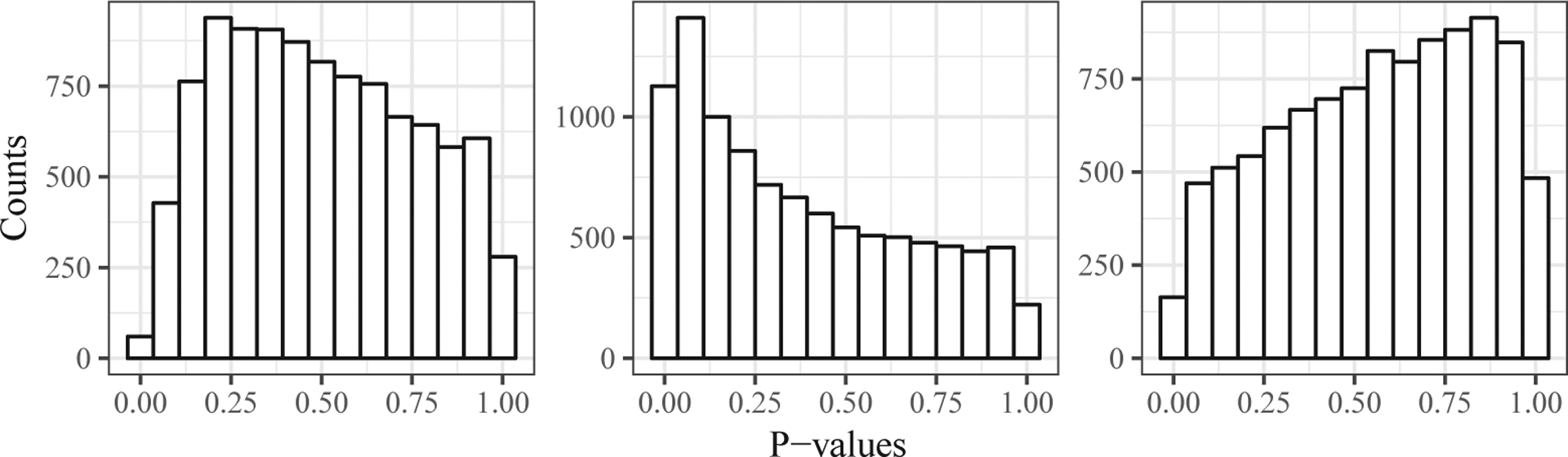
Histograms of p-values from two-sample t-tests when group labels are randomly assigned to samples. Each panel is from a different random seed. The p-value distributions all clearly deviate from uniform.

In recent years, many methods have been introduced to try to solve problems due to unwanted variation. Perhaps the simplest approach is to estimate sources of unwanted variation using a principal components analysis (Price et al. (2006)), and then to control for these factors by using them as covariates in subsequent analyses. Indeed, in genome-wide association studies, this simple method is widely used. However, in gene expression studies, the method suffers from the problem that the principal components will typically also contain the signal of interest, so controlling for them risks removing that signal. To address this, Leek and Storey (2007, 2008) introduced the surrogate variable analysis (SVA), which uses an iterative algorithm to estimate the latent factors that do not include the signal of interest (see also Lucas et al. (2006)). To account for unwanted variation, the SVA assumes a factor-augmented regression model (Section 2.1), which has a long history (and others Fisher and Mackenzie (1923); Cochran (1943); Williams (1952); Tukey (1962); Gollob (1968); Mandel (1969, 1971); Efron and Morris (1972); Freeman (1973); Gabriel (1978)). Since the SVA, numerous similar approaches have emerged, including those of Behzadi et al. (2007), Kang, Ye and Eskin (2008), Carvalho et al. (2008), Kang et al. (2008), Stegle et al. (2008), Friguet, Kloareg and Causeur (2009), Kang et al. (2010), Listgarten et al. (2010), Stegle et al. (2010), Wu and Aryee (2010), Gagnon-Bartsch and Speed (2012), Fusi, Stegle and Lawrence (2012), Stegle et al. (2012), Sun, Zhang and Owen (2012), Gagnon-Bartsch, Jacob and Speed (2013), Mostafavi et al. (2013), Perry and Pillai (2013), Yang et al. (2013), Chen and Zhou (2017), Lee et al. (2017), Wang et al. (2017), McKennan and Nicolae (2020), McKennan and Nicolae (2019), and Gerard and Stephens (2020), among others.

As noted above, a key difficulty in adjusting for unwanted variation in expression studies is distinguishing between the effect of a treatment and the effect of factors correlated with the treatment. Available methods deal with this problem in different ways. Here, we focus on methods that use “negative controls” to help achieve this goal. In the context of a gene expression study, a negative control is a gene whose expression is assumed to be unassociated with all covariates (and treatments) of interest. Under this assumption, negative controls can be used to separate sources of unwanted variation from the treatment effects. The idea of using negative controls in this way appears in Lucas et al. (2006), and was recently popularized by Gagnon-Bartsch and Speed (2012) and Gagnon-Bartsch, Jacob and Speed (2013) in a series of methods and programs known as removing unwanted variation (RUV). There are many RUV methods, including RUV2 (for RUV 2-step), RUV4, RUVinv (a special case of RUV4), RUVrinv, RUVfun, and RUV1.

Understanding the relative merits and properties of the various RUV methods, which all aim to solve essentially the same problem, is a non-trivial task. The main contribution of this study is to present a general framework, RUV*, that encompasses all versions of RUV (Section 4). RUV* represents the problem as a general matrix imputation procedure, providing a unifying conceptual framework, and opening up new approaches based on the large body of literature on matrix imputation. Our RUV* framework also provides a simple and modular way to account for uncertainty in the estimated sources of unwanted variation, which is an issue ignored by most methods. While developing this general framework, we make detailed connections between RUV2 and RUV4, exploiting the formulation in Wang et al. (2017).

On notation: throughout, we denote matrices using bold capital letters (A), except for $\mathit{\alpha }$ and $\mathit{\beta }$, which are also matrices. Bold lowercase letters are vectors $\left(\mathit{a}\right)$, and non-bold lowercase letters are scalars $\left(a\right)$. Where there is no chance for confusion, we use non-bold lowercase to denote scalar elements of vectors or matrices. For example, $a_{ij}$ is the (i, j)th element of A, and $a_i$ is the ith element of $\mathit{a}$. The notation ${\mathit{A}}_{n\times m}$ denotes that the matrix A is an n-by-m matrix. The matrix transpose is denoted by ${\mathit{A}}^{\mathrm{\top }}$, and the matrix inverse is denoted by ${\mathit{A}}^{-1}$. In general, sets are denoted using calligraphic letters $\left(𝓐\right)$, and the complement of a set is denoted with a $\mathrm{b}\mathrm{a}\mathrm{r}\left(\stackrel{-}{𝓐}\right)$.

2. RUV4 and RUV2

2.1. Review of the two-step rotation method

Most existing approaches to this problem (Leek and Storey (2007, 2008); Gagnon-Bartsch and Speed (2012); Sun, Zhang and Owen (2012); Gagnon-Bartsch, Jacob and Speed (2013); Wang et al. (2017)) are based in some way on using a factor analysis (FA) to capture unwanted variation. Specifically, they assume:

$${\mathit{Y}}_{n\times p}={\mathit{X}}_{n\times k}{\mathit{\beta }}_{k\times p}+{\mathit{Z}}_{n\times q}{\mathit{\alpha }}_{q\times p}+{\mathit{E}}_{n\times p},$$ (2.1)

where, in the context of a gene expression study, y_ij is the normalized expression level of the jth gene on the ith sample, X contains the observed covariates, $\mathit{\beta }$ contains the coefficients of X, Z is a matrix of unobserved factors (sources of unwanted variation), $\mathit{\alpha }$ contains the coefficients of Z, and E contains independent (Gaussian) errors with means zero and column-specific variances $\mathrm{v}\mathrm{a}\mathrm{r}\left(e_{ij}\right)={\sigma }_j^2$. In this model, the only known quantities are Y and X.

To fit (2.1), it is common to apply a two-step approach (e.g., Gagnon-Bartsch, Jacob and Speed (2013); Sun, Zhang and Owen (2012); Wang et al. (2017)). The first step regresses out X and then, using the residuals of this regression, estimates $\mathit{\alpha }$ and ${\sigma }_j$. The second step assumes $\mathit{\alpha }$ and ${\sigma }_j$ are known, and estimates $\mathit{\beta }$ and Z. Wang et al. (2017) helpfully frame this two-step approach as a rotation followed by an estimation in two independent models. We now review this approach.

First, let X = QR denote the QR decomposition of X, where $\mathit{Q}\in {\mathbb{R}}^{n\times n}$ is an orthogonal matrix $\left({\mathit{Q}}^{\mathrm{\top }}\mathit{Q}=\mathit{Q}{\mathit{Q}}^{\mathrm{\top }}={\mathit{I}}_n\right)$ and ${\mathit{R}}_{n\times k}={\left({\mathit{R}}_1^{\mathrm{\top }},0\right)}^{\mathrm{\top }}$, where ${\mathit{R}}_1\in {\mathbb{R}}^{k\times k}$ is an upper-triangular matrix. Multiplying (2.1) on the left by ${\mathit{Q}}^{\mathbf{\top }}$ yields

$${\mathit{Q}}^{\mathrm{\top }}\mathit{Y}=\mathit{R}\mathit{\beta }+{\mathit{Q}}^{\mathrm{\top }}\mathit{Z}\mathit{\alpha }+{\mathit{Q}}^{\mathrm{\top }}\mathit{E}.$$ (2.2)

Suppose $k=k_1+k_2$, where the first k₁ covariates of X are not of direct interest, but are included because of various modeling decisions (e.g., an intercept term, or covariates that need to be controlled for). The last k₂ columns of X are the variables of interest, whose putative associations with Y the researcher wishes to test. Let ${\mathit{Y}}_1\in {\mathbb{R}}^{k_1\times p}$ be the first k₁ rows of ${\mathit{Q}}^{\mathbf{\top }}\mathit{Y},{\mathit{Y}}_2\in {\mathbb{R}}^{k_2\times p}$ be the next k₂ rows of ${\mathit{Q}}^{\mathbf{\top }}\mathit{Y}$, and ${\mathit{Y}}_3\in {\mathbb{R}}^{(n-k)\times p}$ be the last n - k rows of ${\mathit{Q}}^{\mathbf{\top }}\mathit{Y}$. Conformably partition ${\mathit{Q}}^{\mathrm{\top }}\mathit{Z}$ into Z₁, Z₂, and Z₃, and ${\mathit{Q}}^{\mathrm{\top }}\mathit{E}$ into E₁, E₂, and E₃. Let

$${\mathit{R}}_1=\left(\begin{array}{cc}{\mathit{R}}_{11}& {\mathit{R}}_{12}\\ 0& {\mathit{R}}_{22}\end{array}\right).$$

Finally, partition $\mathit{\beta }={\left({\mathit{\beta }}_1^{\mathbf{\top }},{\mathit{\beta }}_2^{\mathbf{\top }}\right)}^{\mathbf{\top }}$ so that ${\mathit{\beta }}_1\in {\mathbb{R}}^{k_1\times p}$ contains the coefficients for the first k₁ covariates, and ${\mathit{\beta }}_2\in {\mathbb{R}}^{k_2\times p}$ contains the coefficients for the last k₂ covariates. Then, (2.2) may be written as three models,

$${\mathit{Y}}_1={\mathit{R}}_{11}{\mathit{\beta }}_1+{\mathit{R}}_{12}{\mathit{\beta }}_2+{\mathit{Z}}_1\mathit{\alpha }+{\mathit{E}}_1,$$ (2.3)

$${\mathit{Y}}_2={\mathit{R}}_{22}{\mathit{\beta }}_2+{\mathit{Z}}_2\mathit{\alpha }+{\mathit{E}}_2,$$ (2.4)

$${\mathit{Y}}_3={\mathit{Z}}_3\mathit{\alpha }+{\mathit{E}}_3.$$ (2.5)

Importantly, the error terms in (2.3), (2.4), and (2.5) are mutually independent. This follows from the easily proved fact that E is equal in distribution to ${\mathit{Q}}^{\mathbf{\top }}\mathit{E}$. Thus, the aforementioned two-step estimation procedure changes as follows: first, estimate $\mathit{\alpha }$ and ${\sigma }_j$ using (2.5); second, estimate ${\mathit{\beta }}_2$ and Z₂, given $\mathit{\alpha }$ and ${\sigma }_j$, using (2.4). Equation (2.3) contains the nuisance parameters ${\mathit{\beta }}_1$, and is ignored.

2.2. RUV4

One approach to distinguishing between unwanted variation and effects of interest is to use “control genes” (Lucas et al. (2006); Gagnon-Bartsch and Speed (2012)). A control gene is assumed a priori to be unassociated with the covariate(s) of interest. More formally, the set of control genes, $𝓒\subseteq \{1,\dots ,p\}$, has the property that

$${\beta }_{ij}=0\text{ for all }i=k_1+1,\dots ,k,\text{ and }j\in 𝓒,$$

and is a subset of the truly null genes. Examples of control genes used in practice are spike-in controls (Jiang et al. (2011)), used to adjust for technical factors (e.g., sample batch), and housekeeping genes (Eisenberg and Levanon (2013)), used to adjust for both technical and biological factors (e.g., subject ancestry).

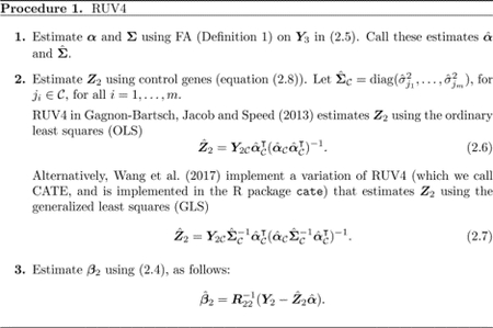
RUV4 (Gagnon-Bartsch, Jacob and Speed (2013)) uses control genes to estimate ${\mathit{\beta }}_2$ in the presence of unwanted variation. Let ${\mathit{Y}}_{2𝓒}\in {\mathbb{R}}^{k_2\times m}$ denote the submatrix of Y₂ with columns that correspond to the m control genes. Similarly, subset the relevant columns to obtain ${\mathit{\beta }}_{2𝓒}\in {\mathbb{R}}^{k_2\times m},{\mathit{\alpha }}_{𝓒}\in {\mathbb{R}}^{q\times m}$, and ${\mathit{E}}_{2𝓒}\in {\mathbb{R}}^{k_2\times m}$. The steps for RUV4, including the variation of Wang et al. (2017), are presented in Procedure 1. (For simplicity, we focus on the point estimates of effects here. For an assessment of the standard errors, see Section S6 of the Supplementary Material.)

The key idea in Procedure 1 is that, for the control genes model (2.4), becomes

$$\begin{gathered} {\mathit{Y}}_{2𝓒}={\mathit{R}}_{22}{\mathit{\beta }}_{2𝓒}+{\mathit{Z}}_2{\stackrel{\mathit{ˆ}}{\mathit{\alpha }}}_{𝓒}+{\mathit{E}}_{2𝓒}, \\ ={\mathit{Z}}_2{\stackrel{\mathit{ˆ}}{\mathit{\alpha }}}_{𝓒}+{\mathit{E}}_{2𝓒}, \end{gathered}$$ (2.8)

$$e_{2𝓒ij}\stackrel{ind.}{~}N\left(0,{\hat{\sigma }}_j^2\right).$$ (2.9)

The equality in (2.8) follows from the property of control genes that ${\mathit{\beta }}_{2𝓒}=0$. Step 2 of Procedure 1 uses (2.8) to estimate Z₂.

Step 1 of Procedure 1 requires an FA of Y₃. We formally define an FA as follows.

Definition 1. A factor analysis (FA), $𝓕$, of rank $q\le \mathrm{m}\mathrm{i}\mathrm{n}(n,p)$ on $\mathit{Y}\in {\mathbb{R}}^{n\times p}$ is a set of three functions $𝓕=\left\{\stackrel{\mathbf{ˆ}}{\mathbf{\Sigma }}\right(\mathit{Y}),\stackrel{\mathit{ˆ}}{\mathit{Z}}(\mathit{Y}),\stackrel{\mathit{ˆ}}{\mathit{\alpha }}(\mathit{Y}\left)\right\}$, such that $\stackrel{\mathbf{ˆ}}{\mathbf{\Sigma }}\left(\mathit{Y}\right)\in {\mathbb{R}}^{p\times p}$ is diagonal with positive diagonal entries, $\stackrel{\mathit{ˆ}}{\mathit{Z}}\left(\mathit{Y}\right)\in {\mathbb{R}}^{n\times q}$ has rank q, and $\stackrel{\mathit{ˆ}}{\mathit{\alpha }}\left(\mathit{Y}\right)\in {\mathbb{R}}^{q\times p}$ has rank q.

RUV4 allows the analyst to choose the FA. Thus, rather than a single method, RUV4 is a collection of methods indexed by the FA used. When we need to be explicit about this indexing, we write $\mathrm{R}\mathrm{U}\mathrm{V}4\left(𝓕\right)$.

2.3. RUV2

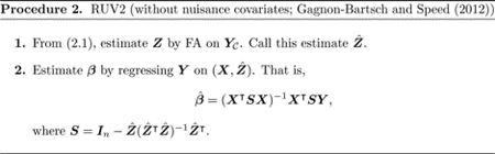
Procedure 2 summarizes the RUV2 method introduced in Gagnon-Bartsch and Speed (2012). It involves two steps: first, estimate the factors causing unwanted variation from the control genes; then, include these factors as covariates in the regression models for the non-control genes. Gagnon-Bartsch, Jacob and Speed (2013) extend this procedure to deal with nuisance covariates by adding a preliminary step that rotates Y and X onto the orthogonal complement of the space spanned by the nuisance covariates (equation (64) in Gagnon-Bartsch, Jacob and Speed (2013)).

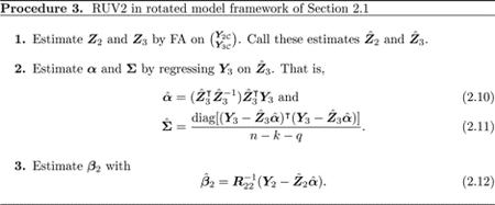
Like RUV4, RUV2 is a class of methods indexed by the FA used, which we here denote by $\mathrm{R}\mathrm{U}\mathrm{V}{2}_{\text{old}}\left(𝓕\right)$. In Procedure 3, we present a method, $\mathrm{R}\mathrm{U}\mathrm{V}{2}_{\text{new}}\left(𝓕\right)$, that we then prove is equivalent to RUV2_old (Theorem 1; proved in Section S2 of the Supplementary Material).

Theorem 1. For a given orthogonal matrix $\mathit{Q}\in {\mathbb{R}}^{n\times n}$ and an arbitrary nonsingular matrix A(Y) that (possibly) depends on Y, suppose

$${𝓕}_1\left(\mathit{Y}\right)=\left\{\hat{\mathit{\Sigma }}\left(\mathit{Y}\right),\hat{\mathit{Z}}\left(\mathit{Y}\right),\hat{\mathit{\alpha }}\left(\mathit{Y}\right)\right\},\mathit{\text{ and }}$$ (2.13)

$${𝓕}_2\left(\mathit{Y}\right)=\left\{\hat{\mathit{\Sigma }}\left({\mathit{Q}}^{\top }\mathit{Y}\right),\mathit{Q}\hat{\mathit{Z}}\left({\mathit{Q}}^{\top }\mathit{Y}\right)\mathit{A}\left(\mathit{Y}\right),{\mathit{A}}^{-1}\left(\mathit{Y}\right)\hat{\mathit{\alpha }}\left({\mathit{Q}}^{\top }\mathit{Y}\right)\right\}.$$ (2.14)

Then,

$$RUV{2}_{\mathit{\text{old}}}\left({𝓕}_2\right)=RUV{2}_{\mathit{\text{new }}}\left({𝓕}_1\right).$$

That is, Procedure 2 using FA (2.13) is equivalent to Procedure 3 using FA (2.14).

The equivalence of RUV2_old and RUV2_new in Theorem 1 involves using different FAs in each procedure. One can ask under what conditions the two procedures would be equivalent if given the same FA. Corollary 1 states that it suffices for the FA to be left orthogonally equivariant (see Section S3 of the Supplementary Material for the proof).

Definition 2. An FA of rank q on $\mathit{Y}\in {\mathbb{R}}^{n\times p}$ is left orthogonally equivariant if

$$\left\{\stackrel{\mathbf{ˆ}}{\mathbf{\Sigma }}\left({\mathit{Q}}^{\mathbf{\top }}\mathit{Y}\right),\stackrel{\mathit{ˆ}}{\mathit{Z}}\left({\mathit{Q}}^{\mathrm{\top }}\mathit{Y}\right)\mathit{A}\left(\mathit{Y}\right),\mathit{A}(\mathit{Y}{)}^{-1}\stackrel{\mathit{ˆ}}{\mathit{\alpha }}\left({\mathit{Q}}^{\mathbf{\top }}\mathit{Y}\right)\right\}=\left\{\stackrel{\mathbf{ˆ}}{\mathbf{\Sigma }}\left(\mathit{Y}\right),{\mathit{Q}}^{\mathbf{\top }}\stackrel{\mathit{ˆ}}{\mathit{Z}}\left(\mathit{Y}\right),\stackrel{\mathit{ˆ}}{\mathit{\alpha }}\left(\mathit{Y}\right)\right\},$$

for all fixed orthogonal $\mathit{Q}\in {\mathbb{R}}^{n\times n}$ and an arbitrary nonsingular $\mathit{A}\left(\mathit{Y}\right)\in {\mathbb{R}}^{q\times q}$ that (possibly) depends on Y.

Corollary 1. Suppose $𝓕$ is a left orthogonally equivariant FA. Then,

$$RUV{2}_{old}\left(𝓕\right)=RUV{2}_{\mathit{\text{new}}}\left(𝓕\right).$$

A well-known FA that is left orthogonally equivariant is the truncated singular value decomposition (formally defined in Section S1 of the Supplementary Material), and this is the only option available in the R package ruv (Gagnon-Bartsch (2015)).

From now on, we use RUV2 to refer to Procedure 3, not Procedure 2, even if the FA is not orthogonally equivariant. (By Theorem 1, this corresponds to Procedure 2 with some other FA.)

3. RUV3

Gagnon-Bartsch, Jacob and Speed (2013) provide a lengthy comparison between RUV2 and RUV4 (their Section 3.4). However, they provide no mathematical equivalencies. We now introduce RUV3, a version of both RUV2 and RUV4. We show that it is the only such procedure that is both RUV2 and RUV4.

3.1. The RUV3 procedure

The main goal in all methods is to estimate ${\mathit{\beta }}_{2\stackrel{-}{𝓒}}$, the coefficients corresponding to the non-control genes. This involves incorporating information from four models, which can be written in matrix form:

$$\left(\begin{array}{ll}{\mathit{Y}}_{2𝓒}& {\mathit{Y}}_{2\stackrel{-}{𝓒}}\\ {\mathit{Y}}_{3𝓒}& {\mathit{Y}}_{3\stackrel{-}{𝓒}}\end{array}\right)=\left(\begin{array}{cc}{\mathit{Z}}_2{\mathit{\alpha }}_{𝓒}+{\mathit{E}}_{2𝓒}& {\mathit{R}}_{22}{\mathit{\beta }}_{2\stackrel{-}{𝓒}}+{\mathit{Z}}_2{\mathit{\alpha }}_{\stackrel{-}{𝓒}}+{\mathit{E}}_{2\stackrel{-}{𝓒}}\\ {\mathit{Z}}_3{\mathit{\alpha }}_{𝓒}+{\mathit{E}}_{3𝓒}& {\mathit{Z}}_3{\mathit{\alpha }}_{\stackrel{-}{𝓒}}+{\mathit{E}}_{3\stackrel{-}{𝓒}}\end{array}\right).$$ (3.1)

The major difference between RUV2 and RUV4 is how the estimation procedures interact in (3.1); see Figure 2 for illustration. RUV2 performs an FA on ${\left({\mathit{Y}}_{2𝓒}^{\mathbf{\top }},{\mathit{Y}}_{3𝓒}^{\mathbf{\top }}\right)}^{\mathrm{\top }}$, then regresses ${\mathit{Y}}_{3\stackrel{-}{𝓒}}$ on the estimated factor loadings. RUV4 performs an FA on $\left({\mathit{Y}}_{3𝓒},{\mathit{Y}}_{3\stackrel{-}{𝓒}}\right)$, then regresses ${\mathit{Y}}_{2𝓒}$ on the estimated factors. The main goal in both, however, is to estimate ${\mathit{Z}}_2{\mathit{\alpha }}_{\stackrel{-}{𝓒}}$, given ${\mathit{Y}}_{2𝓒},{\mathit{Y}}_{3𝓒}$, and ${\mathit{Y}}_{3\stackrel{-}{𝓒}}$.

Figure 2.

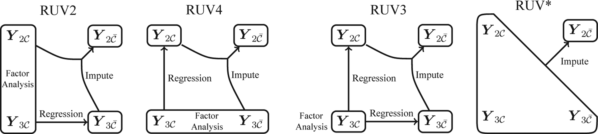
Pictorial representation of the differences between RUV2, RUV4, RUV3, and RUV*.

Estimating ${\mathit{Z}}_2{\mathit{\alpha }}_{\stackrel{-}{𝓒}}$, given ${\mathit{Y}}_{2𝓒},{\mathit{Y}}_{3𝓒}$, and ${\mathit{Y}}_{3\stackrel{-}{𝓒}}$ is, in essence, a matrix imputation problem. In the context of matrix imputation (not removing unwanted variation), Owen and Wang (2016) generalize the methods of Owen and Perry (2009), suggesting that after applying an FA to ${\mathit{Y}}_{3𝓒}$, one should use the estimates ${\stackrel{\mathit{ˆ}}{\mathit{Z}}}_2$ and ${\stackrel{\mathit{ˆ}}{\mathit{\alpha }}}_{\stackrel{-}{𝓒}}$ from (3.2) and (3.3), respectively, and then set $\widehat{{\mathit{Z}}_2{\mathit{\alpha }}_{\stackrel{-}{𝓒}}}={\stackrel{\mathit{ˆ}}{\mathit{Z}}}_2{\stackrel{\mathit{ˆ}}{\mathit{\alpha }}}_{\stackrel{-}{𝓒}}$. This corresponds to an FA, followed by two regressions, followed by an imputation step. Following the theme of this study, we would add an additional step, estimating ${\mathit{\beta }}_{2\stackrel{-}{𝓒}}$ using (3.5).

This estimation procedure (Procedure 4) unifies RUV2 and RUV4, and so we call it RUV3. The unification is formalized in the following theorem (see Section S4 of the Supplementary Material for the proof).

Theorem 2. A procedure is a version of RUV4 (Procedure 1) and RUV2 (Procedure 3) if and only if it is also a version of RUV3 (Procedure 4).

4. A More General Framework: RUV*

A key insight that arises from unifying RUV2 and RUV4 (and RUV3) into a single framework is that they share a common goal: estimating ${\mathit{Z}}_2{\mathit{\alpha }}_{\stackrel{-}{𝓒}}$, which represents the combined effects of all sources of unwanted variation on ${\mathit{Y}}_{2\stackrel{-}{𝓒}}$. This insight suggests a more general approach: any matrix imputation procedure can be used to estimate ${\mathit{Z}}_2{\mathit{\alpha }}_{\stackrel{-}{𝓒}}$; RUV2, RUV3, and RUV4 are just three versions that rely heavily on linear associations between submatrices. Indeed, we need not even assume a factor model for the form of the unwanted variation. Furthermore, we can incorporate uncertainty into the estimates. In this section, we develop these ideas to provide a more general framework for removing unwanted variation, which we call RUV*.

4.1. More general approaches to matrix imputation

To allow for more general approaches to matrix imputation, we generalize (3.1) to

$$\left(\begin{array}{ll}{\mathit{Y}}_{2𝓒}& {\mathit{Y}}_{2\stackrel{-}{𝓒}}\\ {\mathit{Y}}_{3𝓒}& {\mathit{Y}}_{3\stackrel{-}{𝓒}}\end{array}\right)=\left(\begin{array}{ll}\mathbf{\Omega }(\mathit{\varphi }{)}_{2𝓒}& \mathbf{\Omega }(\varphi {)}_{2\stackrel{-}{𝓒}}\\ \mathbf{\Omega }(\varphi {)}_{3𝓒}& \mathbf{\Omega }(\varphi {)}_{3\stackrel{-}{𝓒}}\end{array}\right)+\left(\begin{array}{cc}0& {\mathit{R}}_{22}{\mathit{\beta }}_2\\ 0& 0\end{array}\right)+\mathit{E},$$ (4.1)

where $\mathbf{\Omega }$ is the unwanted variation, parameterized by some $\varphi$. When the unwanted variation is represented by a factor model, we have that $\mathit{\varphi }=\{\mathit{Z},\mathit{\alpha }\}$ and $\mathbf{\Omega }\left(\mathit{\varphi }\right)=\mathit{Z}\mathit{\alpha }$.

The simplest version of RUV* fits this model in two steps:

1. Use any appropriate procedure to estimate ${\mathbf{\Omega }}_{2\stackrel{-}{𝓒}}\left(\mathit{\varphi }\right)$, given $\left\{{\mathit{Y}}_{2𝓒},{\mathit{Y}}_{3𝓒},{\mathit{Y}}_{3\stackrel{-}{𝓒}}\right\}$;

2. Estimate ${\mathit{\beta }}_2$ using

$${\mathit{R}}_{22}^{-1}\left({\mathit{Y}}_{2\stackrel{-}{𝓒}}-{\mathbf{\Omega }}_{2\stackrel{-}{𝓒}}\left(\stackrel{\mathit{ˆ}}{\mathit{\varphi }}\right)\right).$$

This idea is represented in the rightmost panel of Figure 2, and its relationships with the other RUV approaches are illustrated in the Supplementary Material, Figure S1. Rather than restricting factors to being estimated using a linear regression, RUV* allows any imputation procedure to be used to estimate ${\mathbf{\Omega }}_{2\stackrel{-}{𝓒}}\left(\mathit{\varphi }\right)$. This opens up a large body of literature on matrix imputation for use in removing unwanted variation with control genes (e.g., Hoff (2007); Allen and Tibshirani (2010); Candes and Plan (2010); Stekhoven and Bühlmann (2012); van Buuren (2012); Josse, Sardy and Wager (2016)). (Note that RUV* is more general than RUVfun of Gagnon-Bartsch, Jacob and Speed (2013); see Section S5 of the Supplementary Material.)

4.2. Incorporating uncertainty in the estimated unwanted variation

As in previous RUV methods, the second step of RUV* treats the estimate of ${\mathbf{\Omega }}_{2\stackrel{-}{𝓒}}\left(\mathit{\varphi }\right)$ from the first step as if it were “known.” Here, we generalize this, using Bayesian ideas to propagate the uncertainty.

Although using Bayesian methods in this context is not new (Stegle et al. (2008, 2010); Fusi, Stegle and Lawrence (2012); Stegle et al. (2012)), our development shares one of the great advantages of the RUV methods, namely, their modularity. That is, RUV methods separate the analysis into smaller, self-contained steps: the FA step, and the regression step. Modularity is widely used in many fields: mathematicians modularize results using theorems, lemmas, and corollaries; and computer scientists modularize code using functions and classes. Modularity has many benefits, including the following: (i) it is easier to conceptualize an approach if it is broken into small, simple steps; (ii) it is easier to discover and correct mistakes; and (iii) it is easier to improve an approach by improving specific steps. These advantages also apply to developing statistical analyses and methods. For example, using a new method for the FA in an RUV does not require a whole new approach; one simply replaces the truncated SVD with the new FA.

To describe this generalized RUV*, we introduce a latent variable ${\tilde{\mathit{Y}}}_{2\stackrel{-}{𝓒}}$, and write (4.1) as

$$\left(\begin{array}{cc}{\mathit{Y}}_{2𝓒}& {\tilde{\mathit{Y}}}_{2\overline{𝓒}}\\ {\mathit{Y}}_{3𝓒}& {\mathit{Y}}_{3\overline{𝓒}}\end{array}\right)=\Omega \left(\mathit{\varphi }\right)+\mathit{E},$$ (4.2)

$${\mathit{Y}}_{2\overline{𝓒}}={\mathit{R}}_{22}{\mathit{\beta }}_2+{\tilde{\mathit{Y}}}_{2\overline{𝓒}}.$$ (4.3)

Now, consider the following two-step procedure:

1. Use any appropriate procedure to obtain a conditional distribution $h\left({\tilde{\mathit{Y}}}_{2\stackrel{-}{𝓒}}\right)=p\left({\tilde{\mathit{Y}}}_{2\stackrel{-}{𝓒}}\mid {𝓘}_m\right)$, where ${𝓘}_m=\left\{{\mathit{Y}}_{2𝓒},{\mathit{Y}}_{3𝓒},{\mathit{Y}}_{3\stackrel{-}{𝓒}}\right\}$.

2. Perform an inference for ${\mathit{\beta }}_2$ using the likelihood

$$\begin{gathered} L\left({\mathit{\beta }}_2\right) \\ =p\left({\mathit{Y}}_{2\stackrel{-}{𝓒}},{𝓨}_m\mid {\mathit{\beta }}_2\right) \\ =p\left({𝓨}_m\right)\int p\left({\mathit{Y}}_{2\stackrel{-}{𝓒}}\mid {\tilde{\mathit{Y}}}_{2\stackrel{-}{𝓒}},{\mathit{\beta }}_2\right)p\left({\tilde{\mathit{Y}}}_{2\stackrel{-}{𝓒}}\mid {𝓨}_m\right)d{\tilde{\mathit{Y}}}_{2\stackrel{-}{𝓒}}\propto \int \delta \left({\mathit{Y}}_{2\stackrel{-}{𝓒}}-{\tilde{\mathit{Y}}}_{2\stackrel{-}{𝓒}}-{\mathit{R}}_{22}{\mathit{\beta }}_2\right)p\left({\tilde{\mathit{Y}}}_{2\stackrel{-}{𝓒}}\mid {𝓨}_m\right)d{\tilde{\mathit{Y}}}_{2\stackrel{-}{𝓒}} \\ =h\left({\mathit{Y}}_{2\stackrel{-}{𝓒}}-{\mathit{R}}_{22}{\mathit{\beta }}_2\right), \end{gathered}$$

where $\delta (\cdot )$ indicates the Dirac delta function.

Of course, in step 2, one could perform a classical inference for ${\mathit{\beta }}_2$, or place a prior on ${\mathit{\beta }}_2$ and perform a Bayesian inference.

This procedure requires an analytic form for the conditional distribution h. An alternative is to assume that we can sample from this conditional distribution, which yields a convenient sample-based (or “multiple imputation”) RUV* algorithm.

1. Use any appropriate procedure to obtain samples ${\tilde{\mathit{Y}}}_{2\stackrel{-}{𝓒}}^{\left(1\right)},\dots ,{\tilde{\mathit{Y}}}_{2\stackrel{-}{𝓒}}^{\left(t\right)}$ from a conditional distribution $p\left({\tilde{\mathit{Y}}}_{2\stackrel{-}{𝓒}}\mid {𝓘}_m\right)$.

2. Approximate the likelihood for $L\left({\mathit{\beta }}_2\right)$ using the fact that ${\stackrel{\mathit{ˆ}}{\mathit{\beta }}}_2^{\left(i\right)}={\mathit{R}}_{22}^{-1}\left({\mathit{Y}}_{2\stackrel{-}{𝓒}}-\right.\left.{\tilde{\mathit{Y}}}_{2\stackrel{-}{𝓒}}^{\left(i\right)}\right)$ is sampled from a distribution proportional to $L\left({\mathit{\beta }}_2\right)$. (This distribution is guaranteed to be proper; see Section S11 of the Supplementary Material.)

For example, in step 2 we can approximate the likelihood of each element of ${\mathit{\beta }}_2$ using a normal likelihood

$$L\left({\beta }_{2j}\right)\approx N\left({\beta }_{2j};{\hat{\beta }}_{2j},{\hat{s}}_j^2\right),$$ (4.4)

where ${\hat{\beta }}_{2j}$ and ${\hat{s}}_j$ are the mean and standard deviation, respectively, of ${\stackrel{\mathit{ˆ}}{\mathit{\beta }}}_2^{\left(i\right)}$. Alternatively, a t likelihood can be used. Either approach provides an estimate and a standard error for each element of ${\mathit{\beta }}_2$ that accounts for the uncertainty in the estimated unwanted variation. (In contrast, the various methods used by other RUV approaches do not account for this uncertainty; see Section S6 of the Supplementary Material.) Here, we use these values to rank the “significance” of the genes by the value of ${\hat{\beta }}_{2j}/{\hat{s}}_j$. They could also be used as inputs to the empirical Bayes method in Stephens (2017) to obtain measurements of significance related to false discovery rates.

Other approaches to the inference in Step 2 are also possible. For example, given a specific prior on ${\mathit{\beta }}_2$, the Bayesian inference for ${\mathit{\beta }}_2$ could be performed by re-weighting these samples according to this prior distribution (see Section S8 of the Supplementary Material). This re-weighting yields an arbitrarily accurate approximation to the posterior distribution $p\left({\mathit{\beta }}_2\mid {𝓘}_m,{\mathit{Y}}_{2\stackrel{-}{𝓒}}\right)$ (see Section S9 of the Supplementary Material). Posterior summaries using this re-weighting scheme are easy to derive (see Section S12 of the Supplementary Material).

To illustrate the potential for RUV* to produce new RUV methods, we implement a version of RUV* in which we use a Markov chain Monte Carlo scheme to fit a simple Bayesian FA model and, hence, perform the sampling-based imputation in Step 1 of RUV*. See Section S10 of the Supplementary Material for details. We refer to this method as RUVB.

5. Empirical Evaluations

We now compare the methods using simulations based on real data (GTEx Consortium (2015)). The simulation procedure is described in detail in HYPERLINK Section S13 of the Supplementary Material. In brief, we use random subsets of real expression data to create “null data” that contain real (but unknown) “unwanted variation.” Then, we modify these null data to add a known signal. We vary the sample size (n = 6, 10, 20, 40), number of genes (p = 1,000), number of control genes (m = 10, 100), and proportion of null genes $\left({\pi }_0=0.5,0.9,1\right)$.

Being based on real data, these simulations involve realistic levels of unwanted variation. However, they also represent a “best-case” scenario, in which treatment labels are randomized with respect to the factors causing this unwanted variation (see Section S16 of the Supplementary Material for a discussion on the effects of correlated confounding). They also represent a best-case scenario in that the control genes given to each method are simulated to be genuinely null (See Section S17 of the Supplementary Material for a discussion on the effects of misspecifying the negative controls). Even in this best-case scenario, unwanted variation is a major issue, and, as we shall see, obtaining well-calibrated inferences is challenging.

5.1. The methods compared

We compare the standard OLS regression against five other approaches: RUV2, RUV3, RUV4, CATE (the GLS variant of RUV4), and RUVB. In the preceding sections, we focused on how these methods obtain point estimates for ${\mathit{\beta }}_2$. However, in practice, one also needs to find standard errors for these estimates. Just as there are many approaches to producing point estimates, there are many ways of producing standard errors. Here, key techniques include “MAD variance calibration” (Wang et al. (2017)), “control gene variance calibration” (Gagnon-Bartsch, Jacob and Speed (2013)), and empirical Bayes variance moderation (EBVM) (Smyth (2004)); see Section S6 of the Supplementary Material for further detail. Our experience is that the choice of technique can greatly affect the results, particularly the calibration of the interval estimates. We therefore experimented with several approaches to estimating the standard error for each method. We summarize the results by presenting the best-performing version of each method. See Section S15 of the Supplementary Material for more extensive discussion.

For RUVB, we considered two approaches to producing the mean and variance estimates: (i) using sample-based posterior summaries (see Section S12 of the Supplementary Material); and (ii) using the normal approximation to the likelihood in Equation (4.4).

5.2. Comparisons: sensitivity vs. specificity

We compare the power of methods to distinguish null and non-null genes by computing the area under the receiver operating characteristic curve (AUC) for each method, while varying the significance threshold.

The clearest result here is that the methods all consistently outperform the standard OLS (see the Supplementary Material, Figure S3). This emphasizes the benefits of removing unwanted variation in terms of improving the power to detect real effects. For small sample size comparisons (e.g. three vs. three) the gains are smaller, though still apparent, presumably because reliably estimating the unwanted variation is more difficult for small samples.

A second clear pattern is that using EBVM to estimate the standard errors consistently improved the AUC performance: the best-performing method in each family uses EBVM. As might be expected, these benefits are greatest for smaller sample sizes (see the Supplementary Material, Figure S3).

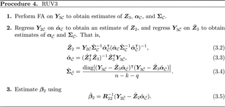
Compared with these two clear patterns, the differences between the best-performing methods in each family are more subtle. Figure 3(a) compares the AUC of the best method in each family with that of RUVB, which performed best overall in this comparison. (The results are shown for ${\pi }_0=0.5$; the results for ${\pi }_0=0.9$ are similar). We highlight four main results:

1. RUVB has the best mean AUC of all methods we explored;

2. The RUV4/CATE methods perform less well (relative to RUVB) when there are few control genes and the sample size is large;

3. In contrast, the RUV2 methods perform less well (relative to RUVB) when the sample size is small and there are few control genes;

4. RUV3 performs somewhat stably (relative to RUVB) across the sample sizes.

Figure 3.

(a) Comparison of AUC achieved by best-performing method in each family versus that of RUVB. Each point shows the observed mean difference in AUC, with vertical lines indicating the 95% confidence intervals for the mean. The results are shown for ${\pi }_0=0.5$, with 10 control genes (upper facet) or 100 control genes (lower facet). All results are below zero (the dashed horizontal line), indicating the superior performance of RUVB. (b) Median coverage for the best-performing methods’ 95% confidence intervals when ${\pi }_0=0.5$. The vertical lines are bootstrap 95% confidence intervals for the median coverage, made transparent and slightly horizontally dodged to increase clarity. The horizontal dashed line is at 0.95. (c) Box plots of the coverage for the best-performing methods’ 95% confidence intervals when ${\pi }_0=0.5$ and $n=40$. For both (b) and (c), the left and right facets show the results for 10 and 100 control genes, respectively.

The mean AUCs for RUVB are given in the Supplementary Material, Figure S2.

5.3. Comparisons: calibration

We also assessed the calibration of the methods by examining the empirical coverage of their nominal 95% confidence intervals for each effect (based on the standard theory for the relevant t distribution in each case).

We begin by examining the “typical” coverage for each method in each scenario by computing the median (across data sets) of the empirical coverage. We find that, without variance calibration, all method families except RUV4/CATE achieve satisfactory typical coverage (somewhere between 0.94 and 0.97) across all scenarios (Figure 3(b) shows the results for ${\pi }_0=0.5$; other values yielded similar results, not shown). The best-performing RUV4/CATE method was often overly conservative in scenarios with few control genes, especially with larger sample sizes.

Although these median coverage results are encouraging, in practice, having small variation in the coverage among data sets is also important. That is, we would like the methods to have near-95% coverage in most data sets, not just on average. Here, the results (Figure 3(c); Supplementary Material, Figure S4) are less encouraging: the coverage of the methods with good typical coverage (median coverage close to 95%) varied considerably among the data sets. Nevertheless, the variability does improve for larger sample sizes and more control genes, and in this case, all methods improve noticeably on the performance of the OLS (Figure 3(c), right facet). Of particular concern is that, across all methods, for many data sets, the empirical coverage can be much lower than the nominal goal of 95%. Such data sets might lead to problems with an over-identification of significant null genes (“false positives”), and an under-estimation of false discovery rates.

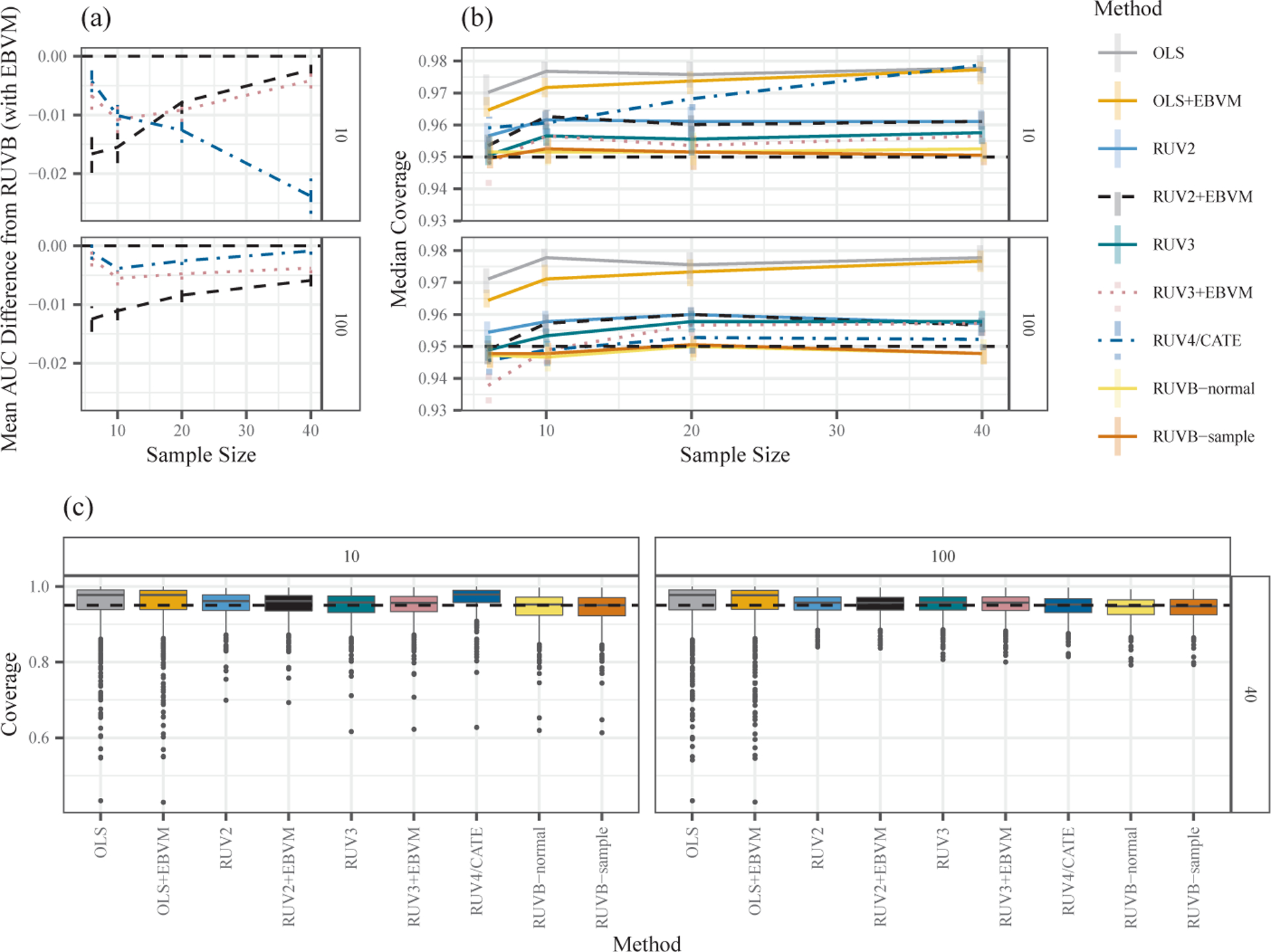
To summarize the variability in coverage—as well as any tendency to be conservative or anti-conservative—we calculated the proportion of data sets in which the actual coverage deviated substantially from 95%, which we defined as being either less than 90% or greater than 97.5%. Figure 4 shows the mean proportions for each method (where the mean was taken over the methods that use each type of variance calibration technique). The key findings are as follows:

1. RUVB (the normal and sample-based versions) exhibits “balanced” errors in coverage: its empirical coverage is as likely to be too high as it is to be too low.

2. MAD calibration tends to produce highly conservative coverage; that is, its coverage is very often much larger than the claimed 95%, and seldom much lower. This tends to reduce false positive significant results, but also substantially reduces the power to detect real effects. The exception is that when all genes are null $\left({\pi }_0=1\right)$, MAD calibration works well for larger sample sizes. These results can be explained partly by the non-null genes biasing the variance calibration parameter upward, an issue also noted in Sun, Zhang and Owen (2012).

3. Control-gene calibration is often anti-conservative when there are few control genes. However, it can work well when the sample size is large and there are many control genes. Interestingly, with few control genes, the anti-conservative behavior gets worse as the sample size increases.

Figure 4.

Mean proportion of times the coverage was either greater than 0.975 (Greater) or less than 0.9 (Less). The column facets distinguish between sample sizes, while the row facets distinguish between the number of control genes and the proportion of genes that are null. The means were taken over the variance calibration method: the MAD calibrated (S6.3), control-gene calibrated (S6.1), or sample- or normal-based RUVB approach.

5.4. Additional simulations

As mentioned earlier, the simulation results in Sections 5.2 and 5.3 are based on a best-case scenario in which the treatment labels are randomized for each individual. To study the effects of correlated confounding, we extended our simulation approach to allow the treatment labels to be correlated with the latent factors (Section S14 of the Supplementary Material). Our results, presented in Section S16 of the Supplementary Material, indicate that RUVB and RUV3 remain competitive in the presence of correlated confounders.

The effects of misspecifying the negative controls are more subtle, as we explore in Section S17 of the Supplementary Material. Our results indicate that RUVB and RUV2 are very sensitive to the negative controls assumption, whereas RUV3 and RUV4 are relatively robust to this assumption (an anonymous reviewer suggested that this might be the result of the regression steps in (2.7) and (3.2)). Thus, we should only use RUVB (and RUV2) when we have high quality negative controls.

References

- Akey JM, Biswas S, Leek JT and Storey JD (2007). On the design and analysis of gene expression studies in human populations. Nature Genetics 39, 807–809. [DOI] [PubMed] [Google Scholar]
- Allen GI and Tibshirani R (2010). Transposable regularized covariance models with an application to missing data imputation. The Annals of Applied Statistics 4, 764–790. [DOI] [PMC free article] [PubMed] [Google Scholar]
- Behzadi Y, Restom K, Liau J and Liu TT (2007). A component based noise correction method (CompCor) for BOLD and perfusion based fMRI. Neuroimage 37, 90–101. [DOI] [PMC free article] [PubMed] [Google Scholar]
- Candes EJ and Plan Y (2010). Matrix completion with noise. Proceedings of the IEEE 98, 925–936. [Google Scholar]
- Carvalho CM, Chang J, Lucas JE, Nevins JR, Wang Q and West M (2008). High-dimensional sparse factor modeling: Applications in gene expression genomics. Journal of the American Statistical Association 103, 1438–1456. [DOI] [PMC free article] [PubMed] [Google Scholar]
- Chen M and Zhou X (2017). Controlling for confounding effects in single cell RNA sequencing studies using both control and target genes. Scientific Reports 7,13587. [DOI] [PMC free article] [PubMed] [Google Scholar]
- Cochran WG (1943). The comparison of different scales of measurement for experimental results. The Annals of Mathematical Statistics 14, 205–216. [Google Scholar]
- Efron B (2004). Large-scale simultaneous hypothesis testing. Journal of the American Statistical Association 99, 96–104. [Google Scholar]
- Efron B (2008). Microarrays, empirical Bayes and the two-groups model. Statistical Science 23, 1–22. [Google Scholar]
- Efron B (2010). Correlated z-values and the accuracy of large-scale statistical estimates. Journal of the American Statistical Association 105, 1042–1055. [DOI] [PMC free article] [PubMed] [Google Scholar]
- Efron B and Morris C (1972). Empirical Bayes on vector observations: An extension of Stein’s method. Biometrika 59, 335. [Google Scholar]
- Eisenberg E and Levanon EY (2013). Human housekeeping genes, revisited. Trends in Genetics 29, 569–574. [DOI] [PubMed] [Google Scholar]
- Fisher RA and Mackenzie WA (1923). Studies in crop variation. ii. the manurial response of different potato varieties. The Journal of Agricultural Science 13, 311–320. [Google Scholar]
- Freeman GH (1973). Statistical methods for the analysis of genotype-environment interactions. Heredity 31, 339–354. [DOI] [PubMed] [Google Scholar]
- Friguet C, Kloareg M and Causeur D (2009). A factor model approach to multiple testing under dependence. Journal of the American Statistical Association 104, 1406–1415. [Google Scholar]
- Fusi N, Stegle O and Lawrence ND (2012). Joint modelling of confounding factors and prominent genetic regulators provides increased accuracy in genetical genomics studies. PLoS Comput Biol 8, e1002330. [DOI] [PMC free article] [PubMed] [Google Scholar]
- Gabriel KR (1978). Least squares approximation of matrices by additive and multiplicative models. Journal of the Royal Statistical Society. Series B (Statistical Methodology) 40, 186–196. [Google Scholar]
- Gagnon-Bartsch J (2015). ruv: Detect and Remove Unwanted Variation using Negative Controls. R package version 0.9.6. [Google Scholar]
- Gagnon-Bartsch J, Jacob L and Speed T (2013). Removing Unwanted Variation from High Dimensional Data with Negative Controls. Technical Report 820, University of California, Berkeley. [Google Scholar]
- Gagnon-Bartsch JA and Speed TP (2012). Using control genes to correct for unwanted variation in microarray data. Biostatistics 13, 539–552. [DOI] [PMC free article] [PubMed] [Google Scholar]
- Gerard D and Stephens M (2020). Empirical Bayes shrinkage and false discovery rate estimation, allowing for unwanted variation. Biostatistics 21, 15–32. [DOI] [PMC free article] [PubMed] [Google Scholar]
- Gibson G (2008). The environmental contribution to gene expression profiles. Nature Reviews Genetics 9, 575–581. [DOI] [PubMed] [Google Scholar]
- Gilad Y and Mizrahi-Man O (2015). A reanalysis of mouse encode comparative gene expression data. F1000Research, 4. DOI: 10.12688/f1000research.6536.1. [DOI] [PMC free article] [PubMed] [Google Scholar]
- Gollob HF (1968). A statistical model which combines features of factor analytic and analysis of variance techniques. Psychometrika 33, 73–115. [DOI] [PubMed] [Google Scholar]
- GTEx Consortium (2015). The Genotype-Tissue Expression (GTEx) pilot analysis: Multitissue gene regulation in humans. Science 348, 648–660. [DOI] [PMC free article] [PubMed] [Google Scholar]
- Hoff PD (2007). Model averaging and dimension selection for the singular value decomposition. Journal of the American Statistical Association 102, 674–685. [Google Scholar]
- Irizarry RA, Warren D, Spencer F, Kim IF, Biswal S, Frank BC et al. (2005). Multiple-laboratory comparison of microarray platforms. Nature Methods 2, 345–350. [DOI] [PubMed] [Google Scholar]
- Jiang L, Schlesinger F, Davis CA, Zhang Y, Li R, Salit M et al. (2011). Synthetic spike-in standards for RNA-seq experiments. Genome Research 21, 1543–1551. [DOI] [PMC free article] [PubMed] [Google Scholar]
- Johnson WE, Li C and Rabinovic A (2007). Adjusting batch effects in microarray expression data using empirical Bayes methods. Biostatistics 8, 118–127. [DOI] [PubMed] [Google Scholar]
- Josse J, Sardy S and Wager S (2016). denoiseR: A package for low rank matrix estimation. arXiv preprint arXiv:1602.01206. [Google Scholar]
- Kang HM, Sul JH, Service SK, Zaitlen NA, Kong S. y., Freimer NB et al. (2010). Variance component model to account for sample structure in genome-wide association studies. Nature Genetics 42, 348–354. [DOI] [PMC free article] [PubMed] [Google Scholar]
- Kang HM, Ye C and Eskin E (2008). Accurate discovery of expression quantitative trait loci under confounding from spurious and genuine regulatory hotspots. Genetics 180, 1909–1925. [DOI] [PMC free article] [PubMed] [Google Scholar]
- Kang HM, Zaitlen NA, Wade CM, Kirby A, Heckerman D, Daly MJ et al. (2008). Efficient control of population structure in model organism association mapping. Genetics 178, 1709–1723. [DOI] [PMC free article] [PubMed] [Google Scholar]
- Lee S, Sun W, Wright FA and Zou F (2017). An improved and explicit surrogate variable analysis procedure by coefficient adjustment. Biometrika 104, 303–316. [DOI] [PMC free article] [PubMed] [Google Scholar]
- Leek JT, Scharpf RB, Bravo HC, Simcha D, Langmead B, Johnson WE et al. (2010). Tackling the widespread and critical impact of batch effects in high-throughput data. Nature Reviews Genetics 11, 733–739. [DOI] [PMC free article] [PubMed] [Google Scholar]
- Leek JT and Storey JD (2007). Capturing heterogeneity in gene expression studies by surrogate variable analysis. PLoS Genetics 3, 1724–1735. [DOI] [PMC free article] [PubMed] [Google Scholar]
- Leek JT and Storey JD (2008). A general framework for multiple testing dependence. Proceedings of the National Academy of Sciences 105, 18718–18723. [DOI] [PMC free article] [PubMed] [Google Scholar]
- Listgarten J, Kadie C, Schadt EE and Heckerman D (2010). Correction for hidden confounders in the genetic analysis of gene expression. Proceedings of the National Academy of Sciences 107, 16465–16470. [DOI] [PMC free article] [PubMed] [Google Scholar]
- Lucas J, Carvalho C, Wang Q, Bild A, Nevins J and West M (2006). Sparse statistical modelling in gene expression genomics. In Bayesian Inference for Gene Expression and Proteomics (Edited by Do K-A, Müller P and Vannucci M), 155–176. Cambridge University Press, Cambridge. [Google Scholar]
- Mandel J (1969). The partitioning of interaction in analysis of variance. Journal of Research of the National Bureau of Standards-B. Mathematical Sciences 73B, 309–328. [Google Scholar]
- Mandel J (1971). A new analysis of variance model for non-additive data. Technometrics 13, 1–18. [Google Scholar]
- McKennan C and Nicolae D (2019). Accounting for unobserved covariates with varying degrees of estimability in high-dimensional biological data. Biometrika 106, 823–840. [DOI] [PMC free article] [PubMed] [Google Scholar]
- McKennan C and Nicolae D (2020). Estimating and accounting for unobserved covariates in high dimensional correlated data. Journal of the American Statistical Association. DOI: 10.1080/01621459.2020.1769635. [DOI] [PMC free article] [PubMed] [Google Scholar]
- Mostafavi S, Battle A, Zhu X, Urban AE, Levinson D, Montgomery SB et al. (2013). Normalizing RNA-sequencing data by modeling hidden covariates with prior knowledge. PloS one 8, 1–10. [DOI] [PMC free article] [PubMed] [Google Scholar]
- Owen AB and Perry PO (2009). Bi-cross-validation of the SVD and the nonnegative matrix factorization. The Annals of Applied Statistics 3, 564–594. [Google Scholar]
- Owen AB and Wang J (2016). Bi-cross-validation for factor analysis. Statistical Science 31, 119–139. [Google Scholar]
- Perry PO and Pillai NS (2013). Degrees of freedom for combining regression with factor analysis. arXiv preprint arXiv:1310.7269. [Google Scholar]
- Price AL, Patterson NJ, Plenge RM, Weinblatt ME, Shadick NA and Reich D (2006). Principal components analysis corrects for stratification in genome-wide association studies. Nature Genetics 38, 904–909. [DOI] [PubMed] [Google Scholar]
- Schwartzman A (2010). Comment. Journal of the American Statistical Association 105, 1059–1063. [DOI] [PMC free article] [PubMed] [Google Scholar]
- Smyth GK (2004). Linear models and empirical Bayes methods for assessing differential expression in microarray experiments. Statistical Applications in Genetics and Molecular Biology 3. DOI: 10.2202/1544-6115.1027. [DOI] [PubMed] [Google Scholar]
- Stegle O, Kannan A, Durbin R and Winn J (2008). Accounting for non-genetic factors improves the power of eQTL studies. In Research in Computational Molecular Biology, 411–422. Springer, Cham. [Google Scholar]
- Stegle O, Parts L, Durbin R and Winn J (2010). A Bayesian framework to account for complex non-genetic factors in gene expression levels greatly increases power in eQTL studies. PLoS Comput Biol 6, e1000770. [DOI] [PMC free article] [PubMed] [Google Scholar]
- Stegle O, Parts L, Piipari M, Winn J and Durbin R (2012). Using probabilistic estimation of expression residuals (PEER) to obtain increased power and interpretability of gene expression analyses. Nature Protocols 7, 500–507. [DOI] [PMC free article] [PubMed] [Google Scholar]
- Stekhoven DJ and Bühlmann P (2012). MissForest—non-parametric missing value imputation for mixed-type data. Bioinformatics 28, 112–118. [DOI] [PubMed] [Google Scholar]
- Stephens M (2017). False discovery rates: a new deal. Biostatistics 18, 275–294. [DOI] [PMC free article] [PubMed] [Google Scholar]
- Sun Y, Zhang NR and Owen AB (2012). Multiple hypothesis testing adjusted for latent variables, with an application to the AGEMAP gene expression data. The Annals of Applied Statistics 6, 1664–1688. [Google Scholar]
- Tukey JW (1962). The future of data analysis. The Annals of Mathematical Statistics 33, 1–67. [Google Scholar]
- van Buuren S (2012). Flexible Imputation of Missing Data. CRC Press, Boca Raton. [Google Scholar]
- Wang J, Zhao Q, Hastie T and Owen AB (2017). Confounder adjustment in multiple hypothesis testing. The Annals of Statistics 45, 1863–1894. [DOI] [PMC free article] [PubMed] [Google Scholar]
- Williams EJ (1952). The interpretation of interactions in factorial experiments. Biometrika 39, 65–81. [Google Scholar]
- Wu Z and Aryee MJ (2010). Subset quantile normalization using negative control features. Journal of Computational Biology 17, 1385–1395. [DOI] [PMC free article] [PubMed] [Google Scholar]
- Yang C, Wang L, Zhang S and Zhao H (2013). Accounting for non-genetic factors by low-rank representation and sparse regression for eQTL mapping. Bioinformatics 29, 1026–1034. [DOI] [PMC free article] [PubMed] [Google Scholar]
Associated Data
This section collects any data citations, data availability statements, or supplementary materials included in this article.