Efficacy of Dynamics-based Features for Machine Learning Classification of Renal Hemodynamics

Abstract

Different machine learning approaches for analyzing renal hemodynamics using time series of arterial blood pressure and renal blood flow rate measurements in conscious rats are developed and compared. Particular emphasis is placed on features used for machine learning. The test scenario involves binary classification of Sprague-Dawley rats obtained from two different suppliers, with the suppliers’ rat colonies having drifted slightly apart in hemodynamic characteristics. Models used for the classification include deep neural network (DNN), random forest, support vector machine, multilayer perceptron. While the DNN uses raw pressure/flow measurements as features, the latter three use a feature vector of parameters of a nonlinear dynamic system fitted to the pressure/flow data, thereby restricting the classification basis to the hemodynamics. Although the performance in these cases is slightly reduced in comparison to that of the DNN, they still show promise for machine learning (ML) application. The pioneering contribution of this work is the establishment that even with features limited to hemodynamics-based information, the ML models can successfully achieve classification with reasonably high accuracy.

I. Introduction

Renal hemodynamics concerns the flow of blood in the vessels of the kidney. In normal circumstances, the kidney’s vasculature responds to blood pressure (BP) variations in a fashion such that renal blood flow (RBF) rate is maintained relatively constant. This renal autoregulation (AR) relates both to the kidney’s function of filtering the blood and also to protection from injury caused by transmission of elevated arterial BP to the sensitive filtering units [12], [20], [24]. The importance of renal AR has led to many investigations into its physiology and characterization from hemodynamic measurements. For instance, the efficiency of AR is considered a major factor influencing the kidney’s susceptibility to hypertensive injury [3], [6]. The capability to assess AR efficiency therefore has investigatory as well as clinical relevance. Indeed, chronic kidney disease (CKD) affects 13.4% of the world’s population [17].

In empirical studies of renal AR in rats and other animals, a variety of techniques has been employed to infer information about AR from BP and RBF measurements. The steady state efficiency of renal AR is most commonly assessed via the Autoregulatory Index (ARI). For the ARI, acute changes in BP are effected using aortic clamps with the animal anesthetized, and the average response in RBF is measured [4], [8], [12], [20]. The response kinetics may also be investigated in such experiments by estimating time constants of (approximately) exponential time courses of the AR response [20].

Another approach to AR assessment utilizes BP and RBF measurements taken either in the anesthetized or conscious state to generate estimates of the empirical transfer function between variational BP and variational RBF [4], [12], [20]. The transfer function estimates, including characteristics of its frequency response, inform about the speed of the AR response [1], [11], [26], the relative contribution of the various mechanisms involved in AR [21], and changes in response to interventions [4], [13]. Nonlinear dynamic models of renal AR, an alternative to the empirical transfer function estimates, obtain higher quality representation of the underlying dynamics [10], [16], capturing some of the nonlinearity known to be extent in renal AR [18].

More recently, calculations akin to the ARI employed with acute BP changes effected under anesthesia have been performed on recordings of BP and RBF obtained in the conscious state using spontaneous fluctuations of BP [5]. These Short Segment ARI (SSARI) values provide improved assessment of AR efficiency when a sufficient number of qualifying pressure change events enable averaging to smooth the inherent variability in the SSARI.

These approaches have had varying degrees of success in elucidating characteristics of AR under experimental conditions. One aspect of the procedures in each case is the determination of specifically conceived features of a dynamic response or description calculated from the hemodynamic time series of BP and RBF. The ARI from step changes in BP, average SSARI values, or values and locations of resonance peaks in the empirical frequency response are examples of this. This present work represents a foray into a different approach, that of machine learning. Rather than defining specific characteristics within the measured data, we let machine learning models draw out the relevant information embedded in the data features presented to them, thereby avoiding any prejudice regarding what aspects are important. We do this in two ways. One approach is the training of a deep neural network (DNN) for which the features presented to it are the raw BP/RBF data record. We first pursued this via a DNN used to assess AR efficiency as intact or impaired [2]. The second approach is to generate a data-determined dynamic input-output model from the variational BP/RBF data and then use the model parameter values as features for the machine learning models. We use the Volterra-FPET model approach of [15], [16] as the best available dynamic representation of the BP/RBF relationship.

With respect to [2], one challenge for network training was that the available data did not allow for clearly labeled training sets. There, groupings of rats were understood to have intact or impaired AR efficiency, dependent on interventions (or the lack thereof) known to affect adversely the function of AR. However, the actual AR efficiency of any single data set was unknown, and hence no data could be definitively labeled as having intact AR or impaired AR. To investigate the efficacy of machine learning to extract information from BP and RBF recordings, we here consider a classification problem in which we do have clearly labeled data.

The Sprague-Dawley (SD) strain of rats has seen much use in the study of renal AR. Investigators have observed that SD rats from two different suppliers, Charles River (CR) and Harlan (Har), present differences in their renal vascular behavior, likely due to effects within the nitric oxide (NO) pathway stemming from genetic drift or possibly contamination within one supplier’s colony [7], [14], [27]. The renal hemodynamics remain otherwise quite similar among all rats of the SD strain. Here we investigate the capability of machine learning models to classify these rats to supplier based on their BP/RBF recordings. Our presumption was that differences connected to NO, a vasodilator, would manifest in the hemodynamic record.

Our approaches using either raw BP/RBF data or the dynamic model parameters as the basic features presented to machine learning models manifest in the following ways. First, a DNN with convolutional and fully connected layers is deployed using raw pressure and flow rate measurements as its features. The DNN performance is compared to that of three other machine learning models: a random forest, a support vector machine, and a multilayer perceptron. Each of these latter three models is presented with a feature vector consisting of parameters from a nonlinear dynamic system fitted to the pressure and flow data. The nature of the feature vector in these cases restricts the classification basis to the dynamic relationship between the pressure and flow, unlike for the DNN. We achieved reasonable classification accuracy by using only the hemodynamic-related features compared to using unrestricted raw information. This pioneering work establishes that ML algorithms can successfully use these dynamics-based features, enabling us to make progress in quantifying CKD based on renal hemodynamic features using ML techniques.

II. Data and Feature Selection

Over the past several decades, the laboratories of several of the authors have produced numerous BP/RBF recordings in SD rats instrumented for chronic monitoring of BP and RBF. These recordings were obtained in support of a variety of experiments over that time, creating a database useful for our machine learning investigations. All animals were cared for in accordance with the Guide for the Care and Use of Laboratory Animals and the protocols approved by the Hines Veterans Affairs Institutional Animal Care and Use Committee. BP time series were acquired from a sensor surgically inserted into the aorta, below the renal artery, with readings communicated via a radiotransmitter as previously described [4], [13]. RBF time series were acquired using an ultrasonic transit time flow probe fitted around the renal artery with the probe cable affixed to the back muscles and exiting the animal at the neck as previously described [4], [13]. A recovery period following the instrumentation surgery precedes data acquisition.

Simultaneous measurement of BP and RBF is done over periods between one and two hours in duration. The data are sampled at 200 Hz, which is adequately fast to avoid aliasing of frequency content in the signals. We have available for each individual rat from one to four such BP/RBF recordings. Within each recording we select 30 minutes of good quality data. The criterion used for assessing data quality is based on an empirical linear transfer function model, developed as described in [13], that relates variational BP to variational RBF. To select the best 30 minute section, we maximize coherence in a frequency range important for the AR dynamics, as described in [2].

The specific data we use in this work come from 230 SD rats from the CR supplier and 87 SD rats from the Har supplier. We partition the rats in each of the two groups into those used for network training (68%), those for validation (7%), and those for testing (25%).

To prepare the data for presentation to the DNN, each 30 minute segment obtained as described above is separated into one minute long snippets of BP and RBF data. Depending on the number of recordings for each rat, we have between 30 and 120 snippets per animal. To diversify the data used for training, the starting sample time for the sequence of snippets is randomized within the first minute of the 30 minute segment. After random selection of this start point, 29 snippets are available for use from that 30 minute segment. Periodically during training, this starting point is randomized again. For test data, we simply used the 30 one minute snippets that occur end to end within the full 30 minute segment. Prior to its input to the network, we normalize the mean and variance of each one minute snippet to zero and one, respectively. These normalizations are performed to prevent classification on the basis of baseline values of BP or RBF and their underlying variability levels. The normalization will not affect the network’s capacity to classify based on relative value changes or the AR dynamics.

For the other machine learning models, the Volterra-FPET modeling approach of [16] was used to generate feature vectors of 456 parameters of models fit to each of the 30 minute data records. This dynamic model produces an estimate of variational RBF as model output, with variational BP as input. The Volterra-FPET provides the best modeling fit amongst all models that have been deployed for this purpose. However, it has seen less use because the model obtained is difficult to interpret. Here, we effectively let the machine learning models do that interpretation. The generated dynamic models use the BP/RBF data resampled to a 2 Hz sampling rate (following appropriate lowpass filtering). In the Volterra-FPET, one selects fixed pole locations that define linear basis systems, appropriate for the modeling situation, with the model output a linear combination of polynomials formed from the basis system outputs. A good choice of fixed poles reduces the overall model complexity, which in this application makes nonlinear AR modeling tractable. We used a complex pole pair at z = 07489 ± j0.4614 with multiplicity two and a real pole at z = 0.9139 with multiplicity eight for a total of 12 poles in the Volterra-FPET. These values represent averages of the values reported in [16], and though not optimized in this setting provide reasonable results when predicting RBF values using the model.

III. Machine Learning Models

We designed the DNN and different machine learning approaches including random forest (RF), support vector machine (SVM), multilayer perceptron (MLP) to classify SD rats based on their two suppliers (CR or Har). These ML approaches were chosen for this work as they are commonly used for renal pathology applications [31]. The models presented were selected after testing with various hyper-parameters. For each ML model, the hyper-parameter tuning is performed using 5-fold cross-validation that combines both training and validation datasets. The optimal values for hyperparameters are selected by performing grid search over the hyperparameter space to strike a balance between model accuracy and overfitting [32].

The DNN structure with three convolutional layers, followed by two fully connected layers is used which is similar to the DNN architectures that have been successfully applied in applications similar to ours [9], [19], [22], [25], [28]–[30]. The input of one-minute-long snippets of BP and RBF data sampled at 200 Hz is presented to first convolutional layer with 16 kernels of length 3 seconds (600 samples). These filters move with a stride of one sample each and operate on the BP and RBF data to learn characteristics of temporal relationship between the two. We follow this with a max pooling layer of shape 10 x 1 that moves with a stride of 2. The second convolutional layer with 24 kernels of shorter length (400 samples), moving with stride of one sample is followed by a max pooling layer of shape 8 x 1 and stride of 2. The third convolutional layer has 32 kernels of length 100 samples, followed again by max pooling (8 x 1, stride of 2). This layer’s output is flattened and fed as input to the first of two fully connected layers. The first fully connected layer has 256 neurons, and the second has 128. All convolutional and fully connected layers use a Rectified Linear Unit (Relu) as the activation function. The second fully connected layer’s output feeds the output layer, which employs a sigmoid activation function with output between 0 (corresponding to CR) and 1 (corresponding to Har). The network architecture for DNN is finalized after extensive variation of different network parameters including number and type of layers, size of input data, number and length of kernels in the convolutional layer and size of the fully connected layers.

The ensemble algorithm of RF model integrating several independent decision trees is used classify the SD rats into the two supplier groups. The 456 feature vectors computed for the 30-minute-long BP and RBF data records generated from Volterra-FPET model discussed in Section 2 are fed to the RF model as input. For RF model, we used 125 decision trees with maximum depth of 6 for each tree. To measure the quality of a split, the entropy criterion is used. The minimum number of samples required to split an internal node and to be at a leaf node are selected as 0.2 and 0.08 of total samples respectively. The output of random forest classifier is obtained by choosing the most popular class amongst the individual decision trees.

Similar to the RF classifier input, the feature vectors obtained as a characterization of Volterra-FPET model are fed to an SVM model to classify the SD rats. SVM is modeled by selecting radial basis function (rbf) as a kernel function. The kernel coefficient for rbf function is selected by considering the input variance and the number of features. Training was sensitive to adjustments of the regularization parameter. We set its value carefully to avoid overfitting.

MLP architecture is analogous to the fully connected layer structure of the DNN model. The features generated from Volterra-FPET model are used as input to the MLP while in case of DNN, convolution layers generate the features from BP and RBF data that are fed to fully connected layers. The first fully connected layer has 256 units, and the second layer has 128 units, similar to the corresponding portions of the DNN network. In both the layers, Relu is used as the activation function and an Adam solver [23] is used for weight optimization. The batch size of 16 with 0.01 strength of regularization term is selected to train the MLP model. It minimizes the cross-entropy loss function and gives a vector of probability estimates per input record. Refinements and improvements of these classification models are expected to be possible.

IV. Training and Testing

We trained the classifier models to distinguish between CR and Har using 156 CR and 59 Har rats. Each rat used for training has one or more 30-minute BP and RBF recordings, all split into successive one-minute snippets for the DNN input. To help diversify training data we randomize the first snippet’s starting point as noted in Section 2. All snippets are normalized to zero mean and unit variance. An additional 16 CR and 6 Har rats are used for validation. We trained the DNN network through multiple epochs to score from 0 (CR) to 1 (Har). As the loss plateaus during training, we reduce the learning rate by four. We used an Adam optimizer [26] to reduce the binary cross entropy loss between the predicted and true classes.

To evaluate the DNN performance after training, we used data from 58 CR and 22 Har rats. Recordings for each rat are broken into a maximum number of one-minute long data snippets. Each snippet is presented to the network, resulting in an output score in the range from 0 to 1. We average the scores for all snippets from a given rat to produce a single score value for that rat. The rat animal gets classified into either CR or Har class depending on the obtained score value.

To train the other ML models, the same training set of 156 CR and 59 Har rats is used. The 456 feature vectors computed for each 30-minute data records generated from Volterra-FPET model is used as input. For a purpose of balancing the training dataset, we divided the CR records into 3 separate bins and kept the Har records same across all bins and trained 3 separate models for each approach considering these bins with same sets of hyperparameters.

For performance evaluation, we used the same 58 CR and 22 Har rats utilized during DNN evaluation. We obtain an output score corresponding to each 30-minute data record, and we classify the record based on this output score.

All these models are trained with five different sets of data partitions for training and testing. This approach helps to achieve a better generalized model performance.

V. Classification Results

The results from the various classification models are presented in terms of accuracy metrics. For a nominal classification threshold of 0.5, we achieved the test accuracy for DNN, RF, SVM, and MLP as 0.902 ± 0.035, 0.828 ± 0.034, 0.757 ± 0.036, and 0.792 ± 0.038 respectively considering all the five data partitions.

Figure 1 shows the receiver operating characteristic (ROC) curves for the best performing classifier models of each type of machine learning model, when presented with the CR and Har test data. We find that the DNN performs the best, while the RF, SVM, and MLP approaches have similar results to each other that are only slightly below the performance of the DNN. The area under the ROC curve (AUC) is shown in Table I. These results give confidence that we can reasonably classify the SD rats into CR and Har classes using these methodologies.

Fig. 1.

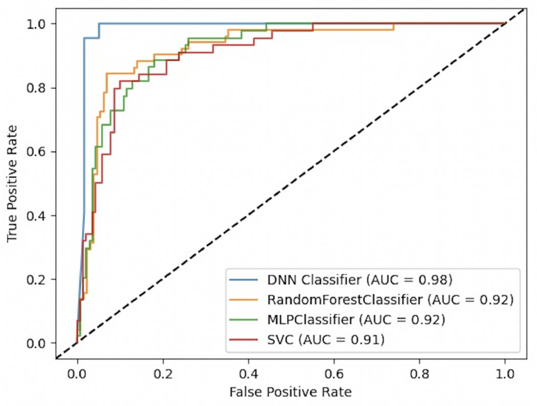
ROC of different models for test data from CR and Har rats.

TABLE I.

AUC of different classifiers

Model Comparison
	DNN	RF	SVM	MLP
AUC	0.98	0.92	0.91	0.92

VI. Discussion and Conclusion

In this study we have demonstrated the capability of machine learning models to distinguish between the CR and Har strains of the SD rat on the basis of BP/RBF measurements. To our knowledge, this is the first study to use dynamics of renal BP and RBF data for animal strain classification, with no previous published work or golden standard to compare against. The accomplishment is not too surprising, given the capabilities of machine learning for such tasks and given that these two strains, though close in most ways, are known to differ in their hemodynamics. Importantly, this capacity to distinguish between the strains is retained when the machine learning models are presented only with the dynamic model relating BP to RBF. Because our interest is to assess the AR capacity, we want to balance between flexibility in the machine learning models with restriction to features that relate to AR.

The DNN models perform best in the classification task. However, information in the BP/RBF record may separate CR from Har for reasons other than AR. The other machine learning models are constrained to act only on the basis of the AR dynamics through the feature vector defined by the nonlinear dynamic model parameters. The fact that the classification performance of these models is lower than that of the DNN suggests the possibility that the DNN was indeed using something other than AR to separate the two strains. One should also keep in mind that the BP/RBF data presented to the DNN was acquired at a 200 Hz sampling rate, which enables utilization of characteristics such as the pulse shape in the BP or RBF record, for instance. Other possibilities are that the AR dynamics only partially separates the two strains, or that the FPET dynamic model captures only imperfectly the AR dynamics.

Nonetheless, we are encouraged that the Volterra-FPET modeling approach of [16] generates a feature vector that provides a basis for effective machine learning analysis of renal AR. We can potentially improve the performance of this approach by further optimizing the selection of the fixed pole locations in the Volterra-FPET, either for groups of records or for individual records. In the latter case the pole locations would become additional features for the machine learning model.

References

- [1].Abu-Amarah I, Bidani AK, Hacıoğlu R, Williamson GA, Griffin KA, “Differential effects of salt on renal hemodynamics and potential pressure transmission in stroke-prone and stroke-resistant spontaneously hypertensive rats,” Am J Physiol Renal Physiol, vol. 289, pp. F305–F313, 2005. [DOI] [PubMed] [Google Scholar]
- [2].Alphonse S, Polichnowski AJ, Griffin KA, Bidani AK, Williamson GA, “Autoregulatory efficiency assessment in kidneys using deep learning,” in Proc 28th European Signal Processing Conference (EUSIPCO), Amsterdam, The Netherlands, January 2021, pp. 1165–1169. [DOI] [PMC free article] [PubMed] [Google Scholar]
- [3].Bidani AK, Griffin KA, “Pathophysiology of hypertensive renal damage: implications for therapy,” Hypertension, vol. 44, pp. 595–601, 2004. [DOI] [PubMed] [Google Scholar]
- [4].Bidani AK, Hacioglu R, Abu-Amarah I, Williamson GA, Loutzenhiser R, Griffin KA, “‘Step’ vs. ‘dynamic’ autoregulation: implications for susceptibility to hypertensive injury,” Am J Physiol Renal Physiol, vol. 285, pp. F113–120, 2003. [DOI] [PubMed] [Google Scholar]
- [5].Bidani AK, Polichnowski AJ, Licea-Vargas H, Long J, Kliethermes S, Williamson GA, and Griffin KA, “BP fluctuations and the realtime dynamics of renal blood flow responses in conscious rats,” J Am Soc Nephrol, 2019. [DOI] [PMC free article] [PubMed] [Google Scholar]
- [6].Bidani AK, Polichnowski AJ, Loutzenhiser R, Griffin KA, “Renal microvascular dysfunction, hypertension and CKD progression,” Curr Opin Nephrol Hypertens, vol. 22, pp. 1–9, 2013. [DOI] [PMC free article] [PubMed] [Google Scholar]
- [7].Buhimschi IA, Shi SQ, Saade GR, Garfield RE, “Marked variation in responses to long-term nitric oxide inhibition during pregnancy in outbred rats from two different colonies,” Am J Obstet Gynecol, vol. 184, pp. 686–693, Mar. 2001. [DOI] [PubMed] [Google Scholar]
- [8].Carlstrom M, Wilcox CS, Arendshorst WJ, “Renal autoregulation in health and disease,” Physiol Rev, vol. 95, pp. 405–511, 2015. [DOI] [PMC free article] [PubMed] [Google Scholar]
- [9].Chambon S, Thorey V, Arnal PJ, Mignot E and Gramfort A, “A deep learning architecture to detect events in EEG signals during sleep,” in Proc 2018 IEEE 28th Int Workshop Machine Learning Signal Processing, Aalborg, pp. 1–6. [Google Scholar]
- [10].Chon KH, Chen Y-M, Holstein-Rathlou N-H, Marmarelis VZ, “Nonlinear system analysis of renal autoregulation in normotensive and hypertensive rats,” IEEE Trans Biomed Eng, vol. 45, no. 3, pp. 342–353, March 1998. [DOI] [PubMed] [Google Scholar]
- [11].Chon KH, Chen YM, Holstein-Rathlou N-H, Marsh DJ, Marmarelis VZ, “On the efficacy of linear system analysis of renal autoregulation in rats,” IEEE Trans Biomed Eng, vol. 40, pp. 8–20, 1993. [DOI] [PubMed] [Google Scholar]
- [12].Cupples WA, Braam B, “Assessment of renal autoregulation,” Am J Physiol Renal Physiol, vol. 292, pp. F1105–1123, 2007. [DOI] [PubMed] [Google Scholar]
- [13].Griffin KA, Hacioglu R, Abu-Amarah I, Loutzenhiser R, Williamson GA, Bidani AK, “Effects of calcium channel blockers on ‘dynamic’ and ‘steady-state step’ renal autoregulation, Am J Physiol Renal Physiol, vol. 286, pp. F1136–F1143, 2004. [DOI] [PubMed] [Google Scholar]
- [14].Griffin K, Polichnowski A, Licea-Vargas H, Picken M, Long J, Williamson G, Bidani A, “Large BP-dependent and -independent differences in susceptibility to nephropathy after nitric oxide inhibition in Sprague-Dawley rats from two major suppliers,” Am J Physiol Renal Physiol, vol. 302, pp. F173–182, 2012. [DOI] [PMC free article] [PubMed] [Google Scholar]
- [15].Hacıoğlu R and Williamson GA, “Reduced complexity Volterra models for nonlinear system identification,” EURASIP J Applied Sig Proc, vol. 2001, pp. 257–265, 2001. [Google Scholar]
- [16].Hacıoğlu R, Williamson GA, Abu-Amarah I, Griffin KA, Bidani AK, “Characterization of dynamics in renal autoregulation using volterra models,” IEEE Trans Biomed Eng, vol. 53, pp. 2166–2176, 2006. [DOI] [PubMed] [Google Scholar]
- [17].Hill NR, Fatoba ST, Oke JL, Hirst JA, O’Callaghan CA, Lasserson DS, Richard Hobbs FD, “Global prevalence of chronic kidney disease - a systematic review and meta-analysis,” PLoS One, vol. 11, no. 7, July 2016. [DOI] [PMC free article] [PubMed] [Google Scholar]
- [18].Holstein-Rathlou N-H, Marsh DJ, “Renal blood flow regulation and arterial pressure fluctuations: A case study in nonlinear dynamics,” Physiological Rev, vol. 74, no. 3, pp. 637–681, July 1994. [DOI] [PubMed] [Google Scholar]
- [19].Joshi SR, Headley DB, Ho KC, Paré D, Nair SS, “Classification of brainwaves using convolutional neural network,” in Proc 2019 27th European Signal Processing Conf, A Coruna, Spain, 2019, pp. 1–5. [DOI] [PMC free article] [PubMed] [Google Scholar]
- [20].Just A, “Mechanisms of renal blood flow autoregulation: dynamics and contributions,” Am J Physiol Regul Integr Comp Physiol, vol. 292, pp. R1–17, 2007. [DOI] [PubMed] [Google Scholar]
- [21].Just A, Arendshorst WJ, “Dynamics and contribution of mechanisms mediating renal blood flow autoregulation,” Am J Physiol Regul Integr Comp Physiol, vol. 285, pp. R619–R631, 2003. [DOI] [PubMed] [Google Scholar]
- [22].Kashiparekh K, Narwariya J, Malhotra P, Vig L and Shroff G, “ConvTimeNet: a pre-trained deep convolutional neural network for time series classification,” in Proc 2019 Int Joint Conf Neural Networks, Budapest, Hungary, pp. 1–8. [Google Scholar]
- [23].Kingma DP, Ba JL, “Adam: a method for stochastic optimization,” in Proc 3rd Int Conf Learning Representations, San Diego CA, 2015. [Google Scholar]
- [24].Loutzenhiser R, Griffin K, Williamson G, Bidani A, “Renal autoregulation: new perspectives regarding the protective and regulatory roles of the underlying mechanisms,” Am J Physiol Regul Integr Comp Physiol, vol. 290, pp. R1153–R1167, 2006. [DOI] [PMC free article] [PubMed] [Google Scholar]
- [25].Matsui S, Inoue N, Akagi Y, Nagino G, Shinoda K, “User adaptation of convolutional neural network for human activity recognition,” in Proc 25th European Signal Processing Conf, Kos, Greece, 2017, pp. 753–757. [Google Scholar]
- [26].Pires SL, Barres C, Sassard J, Julien C, “Renal blood flow dynamics and arterial pressure lability in the conscious rat,” Hypertension vol. 38, pp. 147–152, 2001. [DOI] [PubMed] [Google Scholar]
- [27].Pollock DM, Rekito A, “Hypertensive response to chronic NO synthase inhibition is different in Sprague-Dawley rats from two suppliers,” Am J Physiol Regul Integr Comp Physiol, vol. 275, pp. R1719–1723, Nov. 1998. [DOI] [PubMed] [Google Scholar]
- [28].Şen SY and Özkurt N, “ECG Arrhythmia Classification By Using Convolutional Neural Network And Spectrogram,” in Proc 2019 Innovations in Intelligent Systems and Applications Conf, Izmir, Turkey, 2019, pp. 1–6. [Google Scholar]
- [29].Weng S, Li W, Zhang Y and Lyu S, “Dual-stream CNN for structured time series classification,” in Proc 2019 IEEE Int Conf Acoustics, Speech and Signal Processing, Brighton, United Kingdom, pp. 3187–3191. [Google Scholar]
- [30].Zhao B, Lu H, Chen S, Liu J, Wu D, “Convolutional neural networks for time series classification,” J Syst Eng Electron, vol. 28, no. 1, pp. 162–169, 2017. [Google Scholar]
- [31].Magherini R, Mussi E, Volpe Y, Furferi R, Buonamici F, Servi M, “Machine Learning for Renal Pathologies:An Updated Survey,” Sensors, Basel, Switzerland, vol. 22 no. 13(4989), Jul. 2022. [DOI] [PMC free article] [PubMed] [Google Scholar]
- [32].Pedregosa F, Varoquaux G, Gramfort A, Michel V, Thirion B, Grisel O, Blondel M, Prettenhofer P, Weiss R, Dubourg V, Vanderplas J, Passos A, Cournapeau D, Brucher M, Perrot M, Duchesnay E,“Scikit-learn: Machine learning in Python,” Journal of machine learning research, vol. 12, pp. 2825–2830, 2011. [Google Scholar]