Correlating Deep Learning-Based Automated Reference Kidney Histomorphometry with Patient Demographics and Creatinine

Abstract

Key Points

• The authors leverage the unique benefits of panoptic segmentation to perform the largest ever quantitation of reference kidney morphometry.

• Kidney features vary with age and sex; and glomeruli size may intricately link to creatinine, defying prior notions.

Background

Reference histomorphometric data of healthy human kidneys are largely lacking because of laborious quantitation requirements. Correlating histomorphometric features with clinical parameters through machine learning approaches can provide valuable information about natural population variance. To this end, we leveraged deep learning (DL), computational image analysis, and feature analysis to associate the relationship of histomorphometry with patient age, sex, serum creatinine (SCr), and eGFR in a multinational set of reference kidney tissue sections.

Methods

A panoptic segmentation neural network was developed and used to segment viable and sclerotic glomeruli, cortical and medullary interstitia, tubules, and arteries/arterioles in the digitized images of 79 periodic acid–Schiff-stained human nephrectomy sections showing minimal pathologic changes. Simple morphometrics (e.g., area, radius, density) were quantified from the segmented classes. Regression analysis aided in determining the association of histomorphometric parameters with age, sex, SCr, and eGFR.

Results

Our DL model achieved high segmentation performance for all test compartments. The size and density of glomeruli, tubules, and arteries/arterioles varied significantly among healthy humans, with potentially large differences between geographically diverse patients. Glomerular size was significantly correlated with SCr and eGFR. Slight, albeit significant, differences in renal vasculature were observed between sexes. Glomerulosclerosis percentage increased, and cortical density of arteries/arterioles decreased, as a function of increasing age.

Conclusions

Using DL, we automated precise measurements of kidney histomorphometric features. In the reference kidney tissue, several histomorphometric features demonstrated significant correlation to patient demographics, SCr, and eGFR. DL tools can increase the efficiency and rigor of histomorphometric analysis.

Introduction

Diagnostic renal pathology relies on recognizing histologic findings that deviate from the expected range for normal or healthy tissue, hereby defined as reference tissue with none to minimal histopathologic abnormality. Existing morphometrics were commonly measured manually from autopsy specimens, and living-donor samples of reference kidney tissue remain difficult to obtain because tissue samples are not typically taken from healthy patients. In addition, detailed reference histomorphometric data of healthy human kidneys are largely lacking because of laborious quantitation requirements. With recent advances in the technical capabilities and performance of deep learning (DL)-based image analysis, computational pathology has emerged as a potential feasible and scalable method to automate histomorphometric quantitation and provide accurate reference kidney histomorphometric data. If applied to a large and diverse sample of healthy human kidneys, this approach can provide insights into histomorphometric natural variance within populations and subgroups, which may correlate to clinical parameters and disease susceptibility. Similar detailed quantitation in disease states may provide additional diagnostic and prognostic information that are not currently available or feasible for routine diagnostic renal pathology practice. However, the utility of such data can only be recognized if reliable reference values are available for comparison.

In this study, we developed a DL-based image analysis model for conducting comprehensive segmentation of renal histomorphometry and applied it to whole slide images (WSIs) of reference kidney tissue to automate the measurement of simple histomorphometric features. These quantified features were then correlated to patient demographics, serum creatinine (SCr), and eGFR values to assess their biological relevance.

Methods

This study was approved by the institutional review board at the University of Florida with waiver of informed consent.

Kidney Tissue Sections

All deidentified kidney tissue sections in this study were obtained from the pathology archives of the University of California, Davis, Centro Hospitalar e Universitário de Coimbra, and Seoul National University Hospital. The original tissue was formalin-fixed, paraffin-embedded, and sectioned at 2–4 µm in thickness. The cases and stains used are detailed below.

Image Data

WSIs were generated by scanning the glass slides with a whole slide brightfield microscopy image scanner (Aperio, Leica, CA). Spatial annotation of tissue sections was performed in Aperio ImageScope and saved as ImageScope compatible XML files.

Training Data

For segmentation training, 190 WSIs were collected, including 53 diabetic nephropathy, 39 lupus nephritis, and 11 transplant surveillance needle core biopsies (total tissue area, 1100 mm²), 58 large sub-WSIs manually cropped from healthy portions of 33 reference kidneys (total tissue area 369 mm²), 23 small sub-WSIs of five hematoxylin and eosin needle core biopsies (total tissue area 34 mm²), two small sub-WSIs from a silver-stained biopsy (2 mm²), and four sub-WSIs from a trichrome biopsy (1.4 mm²). Samples were collected from a variety of institutions and disease types to create a diverse image set for model training. Diverse training data improve the robustness of the model to holdout slides from different institutions and disease states, such as those included in this study. These slides were annotated in their entirety for viable and sclerotic glomeruli, cortical and medullary interstitia, tubules, and arteries/arterioles. Overall, 1506 mm² of kidney tissue was annotated.

Performance Analysis and Ground-Truth Data

Ten periodic acid–Schiff (PAS) transplant surveillance kidney biopsy sections (nine needle cores, one wedge) were used for performance measurement. Five patients had SCr at the time of biopsy of >2 mg/dl, and five patients were selected to have histologically normal biopsy findings as per the original case report to measure performance both in diseased and healthy states. This choice was made to ensure that the model performs well in a variety of holdout samples because none of these slides were included in training the algorithm. Glomeruli <1500 µm² in the area and glomerular fragments that were not physically contiguous with the biopsy core were not considered. Very small diameter arterioles were difficult to discern from capillaries; therefore, the smallest vessels annotated as arterioles for the purpose of performance evaluation were those >200 µm² in area and displaying at least one full circumferential layer of smooth muscle cells, barring the loss of smooth muscle to disease. The smallest annotatable tubule was also defined as those >200 µm² in area because below this threshold, the objects could not be confidently determined as tubules. The area thresholds discussed herein were applied to the neural network segmentation outputs to filter the structures for performance evaluation.

Reference Kidney Data

The reference kidney tissue sections consisted of archived glass slides of the renal parenchyma uninvolved and away from the renal tumor of human tumor nephrectomy specimens. These cases were screened to have no evidence of hydronephrosis, infectious disease, or proteinuria. The renal pathologist screened the slides to include only cases with minimal pathologic changes (e.g., no tumor, no significant preservation or processing artifact, and <5% interstitial fibrosis and tubular atrophy). These criteria were implemented to ensure that only areas of tissue consistent with reference morphometry were included. In total, reference sections from 79 unique participants were included, with a tissue area totaling 17,208 mm². eGFR was measured using the 2021 CKD Epidemiology Collaboration eGFRcr equation.¹

Renal Multicompartment Segmentation

Tissue Detection

The renal tissue regions were detected from the background by creating a low-resolution thumbnail (16× downsample) of the entire WSI and transforming it to the hue, saturation, and value color space. From the resultant image, the total tissue area was measured by thresholding the saturation channel at 0.05, summing all the pixels in the resultant binary mask, and converting the output to mm². To identify image regions of tissue for DL processing, the saturation channel was further blurred with a Gaussian filter (σ=5) to create a loose buffer zone around the tissue edge. The blurred saturation image was converted to a binary mask by thresholding at 0.05. This low-resolution mask was gridded into a set of tiles on the basis of the desired training or testing patch size for renal multicompartment segmentation, amount of overlap between patches, and tolerable percent of nontissue per patch. For training, image size was specified as 1200×1200 pixels, and an overlap of 50% between adjacent tiles was allowed. For testing, image size was specified as 2048×2048 pixels, with 10% overlap between patches. For both training and testing, any tile with >99% background was excluded from further processing.

Data Loading for DL

Network training was orchestrated using the Detectron2 library for PyTorch, which implements convenient functions for training and evaluating a panoptic feature pyramid architecture. A custom data loader to extract image crops and associated labels from WSIs and XMLs was designed to feed network training on the fly rather than saving image crops to disk, resulting in reduced memory overhead and disk usage, as well as allowing the added convenience of implementing balanced data sampling routines both at the whole-slide and target-class levels.

Given that the cross-sectional area of kidney tissue sections consists of mostly tubules, a data selection routine for class balance was required to prevent an underfit classifier on nontubule targets and performed as follows: For each patch requested during training, one slide from the training set was selected randomly. Next, with a 50% probability, either a random slide tile was extracted from the tissue area or the tile was selected to be centered on a randomly selected artery/arteriole or glomerulus. All random sampling was performed using a uniform distribution.

Training

Network weights were initialized to a model pretrained on the Common Objects in COntext (COCO) dataset available in the Detectron2 library, which had a ResNet-50 backbone and was originally trained with the 3× learning rate schedule. The following modifications were made to the network architecture, which differed from the stock configuration of Detectron2: The anchor generator sizes were specified as 32, 64, 128, 256, 512, and 1024; the respective region proposal network's input layers for these anchors were specified as p2, p3, p4, p5, p6, and p6; the anchor generator aspect ratios were specified as 0.1, 0.2, 0.33, 0.5, 1, 2, 3, 5, and 10; and the anchor generator angles were specified as −90, −60, −30, 0, 30, 60, and 90. No image resizing was performed, and training was performed with batch size four and region of interest head batch size 64. Several image augmentations were performed to improve network robustness to unseen test variations (further discussed in the Supplemental Material). A similar training schedule was followed as was laid out in the original implementation² for training on the COCO dataset. Starting from the COCO pretrained model, the network was trained for a total of 350 thousand steps, with a step learning rate policy starting at 0.0025 and dropping by one tenth on reaching 100 thousand, 200 thousand, and 300 thousand steps. Glomeruli (viable and sclerotic), tubules, and arteries/arterioles were specified as instance-type segmentation objects, and the interstitium and slide background were specified as semantic-type segmentation objects.

Testing

The custom data loader described in section Data Loading for DL was repurposed for prediction on test biopsy data by converting its output to yield each tile in a WSI grid once. Tiles were sent to the trained DL network for prediction, and the corresponding predictions filled into a high-resolution segmentation mask within the WSI. Predictions in overlapped regions of tiles were resolved by clipping the trailing and leading edges of overlap halfway. In addition, the panoptic network's region of interest head (see refs. 2 and 3 for further details) threshold was set to 0.01 to maximize the number of detected instances. All objects in the final high-resolution mask were converted to their corresponding boundary contour vertices and stored in an XML file compatible with Aperio ImageScope (Leica Biosystems, Nussloch, Germany) or in JSON files compatible with HistomicsUI.

Segmentation Performance Analysis

Multicompartment segmentation performance was assessed both pixel-wise and instance-wise for a comprehensive performance evaluation of our DL pipeline.

Pixel-wise Performance Analysis

Whole-slide manual annotations of the instance segments were compared pixel-wise against network output whole-slide predictions for each class using a one-versus-all approach. Manual annotations for all test slides were completed by one renal pathologist. The true/false positive/negative pixels were pooled across the entire dataset to calculate the final reported performance values, including sensitivity, specificity, precision, negative predictive value, Matthew correlation coefficient, and Dice coefficient.

Instance-Wise Performance

Instance performance calculations were evaluated in the cortex of each WSI only because medulla is not used routinely for diagnostic purposes. Network-predicted instances were annotated with a dot marker if the prediction was incorrect for any reason. The types of error for each instance prediction were broken down into fused instances, partially detected instances, missed instances, and wrong classifications and counted at the WSI level. Partial, fused, and false class percentage error rates were calculated as $\frac{\#errors}{\#predictions}$. Missed percentage error rates were calculated as $\frac{\#misses}{\#misses+\#predicted}$. Total error rate was calculated as $\frac{\#total\hspace{0.17em}errors}{\#predicted+\#misses}$, where #total errors were defined as the sum of #errors and #misses.

Reference Kidney Morphometry

Reference kidney morphometrics were quantified using the saved contour representation of segmented object boundaries for each WSI. The full list of tested features is available in the Supplemental Material. A generic overview of our object feature quantification strategy is discussed below. Note that any glomerular predictions contained within medulla were algorithmically eliminated.

Object Diameter

Calculation of diameters for segmented spherical objects (i.e., glomeruli) is straightforward. Diameter measurements of nonspheroid objects (e.g., tubules and vessels) are complex and subject to bias. Thus, an automated method that can measure object diameters and minimize sampling bias but maximize application to various sectioned orientations of histologic structures was developed, reliant on a morphometric processing method called distance transform. The distance transform takes each object pixel and measures the distance to the closest boundary point. The result at every pixel describes the largest radius of a circle centered at that pixel and inscribed within the object. The maximum of all these pixel values is the radius of the largest circle that is inscribed within the object. We defined tubular and vessel diameter using the diameter of the largest circle. The Supplemental Figure 1 discusses examples of the distance transformation for varied tubule segments.

Object Area

Segmented object areas were calculated from contour vertices using Green's theorem.⁴ To compute the cortical interstitial area, the aggregate area of objects contained within the cortex (i.e., glomeruli, tubules, and arteries/arterioles) was subtracted from the total cortical area. Similarly, the medullary interstitial area was calculated by subtracting the aggregate area of medullary tubules from the total medullary area.

Object Densities

Enumeration and quantification of segmented objects were normalized to the total tissue area that contained the objects, which represents respective object densities. The simplest of these metrics was the division of the number of counted glomeruli, tubules, or arteries/arterioles or their summed areas, by the observed area over which they were distributed (either cortical area, medullary area, or both). To compute the interstitial density, the calculated cortical or medullary interstitial areas were divided by the total cortical or medullary contour areas, respectively.

Arterial/Arteriolar Luminal Ratio

Arterial/arteriolar luminal ratio was calculated as the radius of the artery/arteriole lumen divided by the radius of the entire segmented vessel. To identify the luminal area, the corresponding red green blue image region for each artery/arteriole segmentation was extracted, transformed to LAB colorspace, and the lightness channel of the LAB colorspace was thresholded at 70, yielding a segmentation of the white regions in the vessel. Vessels with overall image width or height >5000 pixels were excluded from this analysis because of the network commonly detecting these vessels as fragments, limiting the ability to properly segment lumina.

Statistical Analysis

Instance-level features were aggregated to the subject level by calculating density, averages, and SDs. Differences in subject-level features across institutions are shown in Table 1 and Supplemental Table 1. The Fisher's exact test was used to test independence for categorical variables, while the ANOVA was used to test differences across institutions for continuous variables. Bonferroni correction was used to adjust for multiple comparisons.⁵

Table 1.

Reference morphometrics (N=79 participants; one whole-slide image per participant)

Reference Morphometrics	Institution 1 (n=43)	Institution 2 (n=8)	Institution 3 (n=28)	Combined (N=79)
Patient characteristics
Male sex, n (%)	29 (67.44)	5 (62.50)	20 (71.43)	54 (68.35)
Age, yr	59.16±11.95	60.63±13.32	53.68±11.94	57.37±12.25
SCr, mg/dl	1.07±0.24	0.81±0.28a	0.86±0.14a	0.97±0.24
Glomerular histomorphometric
Glomeruli, per cortical mm2	2.59±0.64	1.86±0.57a	2.57±0.80b	2.51±0.72
Sclerotic glomeruli, per cortical mm2	0.19±0.14	0.08±0.06	0.24±0.21	0.20±0.17
Glomerular proportion of cortex	0.05±0.01	0.04±0.01	0.05±0.01	0.05±0.01
Average glomerular area, µm2	18,833±3765	23,836±6113a	19,248±3361b	19,487±4134
SD glomerular area, µm2c	9653±3879	10,863±2699	8451±1846	9350±3242
Average glomerular radius, µm	63.8±6.81	72.08±10.73a	65.93±5.98	65.39±7.33
SD glomerular radius, µm	17.08±2.63	19.62±3.74	16.88±2.94	17.27±2.93
Average sclerotic glomerular area, µm2	8252±1712	9222±1883	7780±1579	8188±1713
SD sclerotic glomerular area, µm2	4159±1325	5293±3085	2797±1319a,b	3804±1751
Average sclerotic glomerular radius, µm	42.04±4.66	44.69±5.13	42.62±4.68	42.51±4.72
SD sclerotic glomerular radius, µm	11.56±2.03	13.03±3.45	8.33±3.89a,b	10.59±3.37
Glomerulosclerosis ratio	0.07±0.06	0.04±0.04	0.08±0.07	0.07±0.06
Tubular morphometrics
Tubules, per cortical mm2	173.53±34.40	132.92±38.17a	189.58±50.16b	175.10±43.57
Tubular proportion of cortex	0.55±0.05	0.52±0.07	0.45±0.09a,b	0.51±0.08
Average cortical tubular area, µm2	3269±612	4219±1141a	2476±722a,b	3084±885
SD cortical tubular area, µm2	3495±1002	5752±3652a	2809±1232b	3481±1719
Average cortical tubular radius, µm	20.95±1.53	23.43±2.39a	17.92±2.31a,b	20.13±2.62
SD cortical tubular radius, µm	7.65±1.02	8.93±1.67a	7.00±1.38b	7.55±1.33
Cortical glomerulus to tubule ratio	0.09±0.02	0.08±0.02	0.11±0.02a,b	0.09±0.02
Vascular morphometrics
Arteries(ioles), per cortical mm2	5.96±1.59	4.04±1.14a	6.54±1.98b	5.97±1.82
Arter(iole) proportion of cortex	0.04±0.02	0.03±0.01	0.04±0.02	0.04±0.02
Average lumen to wall ratio	0.27±0.05	0.37±0.05	0.23±0.04a,b	0.27±0.06

Data are represented as mean±SD, if not indicated otherwise. SCr, serum creatinine.

^aAdjusted P value ≤ 0.05 compared with institution 1.

^bAdjusted P value ≤ 0.05 compared with institution 2.

^cSD for the population of glomeruli within a single case.

Multivariable linear regression analyses were performed to assess adjusted associations between each subject-level morphometric feature and age, sex, and SCr. Additional models were used to assess associations between each feature and eGFR after controlling for age and sex. Standard errors were calculated using a cluster robust method to account for individuals being clustered within institutions.⁶ Fixed effects per institution were included in all models. All statistical analyses were performed in R. Coefficients, 95% confidence intervals, and their significance are shown in Table 2.

Table 2.

Association of reference morphometrics to age, sex, serum creatinine, and eGFR

Outcome (R2)	Age		Sex		SCr		eGFR
	β (95% CI)	P Value	β (95% CI)	P Value	β (95% CI)	P Value	β (95% CI)	P Value
Glomerular histomorphometric
Mean glomerular area, µm2 (0.31)	14.2 (−68.6 to 97.1)	0.733	1685.5 (774.2 to 2596.7)a	<0.001a	5826.4 (4258.3 to 7394.5)a	<0.001a	−51.0 (−74.0 to −28.1)a	<0.001a
Mean glomerular radius, µm (0.31)	0.02 (−0.14 to 0.18)	0.805	2.96 (1.10 to 4.82)a	0.002a	10.94 (7.53 to 14.35)a	<0.001a	−0.101 (−0.149 to −0.053)a	<0.001a
SD glomerular area, µm2 (0.09)	17.8 (−14.9 to 50.6)	0.282	1486.9 (1164.2 to 1809.5)a	<0.001a	−1300.7 (−1746.1,−855.3)a	<0.001a	23.6 (−0.81 to 47.92)b	0.058b
Glomerular area density (0.05)	0 (−0.0001 to 0.0001)	0.876	0.001 (−0.003 to 0.005)	0.581	−0.006 (−0.008 to −0.005)a	<0.001a	0 (0.000 to 0.001)a	<0.001a
Glomeruli, per cortical cm2 (0.21)	−0.001 (−0.430 to 0.430)	0.996	−17.53 (−37.53 to 2.47)b	0.085b	−90.7 (−120.7 to −60.7)a	<0.001a	0.640 (0.313 to 0.967)a	<0.001a
Sclerotic glomeruli, per cortical cm2 (0.23)	0.570 (0.090 to 1.051)c	0.021c	1.728 (−2.002 to 5.458)	0.359	0.372 (−27.956 to 28.699)	0.979	0.015 (−0.248 to 0.278)	0.909
Mean sclerosed glomerular radius, µm (0.05)	0.046 (−0.096 to 0.187)	0.523	−0.407 (−1.92 to 1.1)	0.593	2.735 (2.555 to 2.914)a	<0.001a	−0.013 (−0.017 to −0.009)a	<0.001a
Glomerulosclerosis ratio (0.18)	0.0018 (0.0007 to 0.0021)a	0.002a	0.013 (0.002 to 0.025)a	<0.001a	0.031 (−0.062 to 0.123)	0.511	−0.0002 (−0.001 to 0.001)	0.600
Tubular morphometrics
Cortical tubular area density (0.34)	0.0003 (−0.0022 to 0.0028)	0.806	−0.008 (−0.044 to 0.027)	0.642	0.084 (0.035 to 0.133)a	0.001a	−0.001 (−0.001 to 0.000)c	0.016c
Mean cortical tubular area, µm2 (0.43)	−5.84 (−30.87 to 19.20)	0.643	12.20 (−554.5 to 578.9)	0.966	1018.9 (470.9 to 1566.9)a	<0.001a	−7.52 (−16.00 to 0.96)b	0.081b
Mean cortical tubular radius, µm (0.55)	0.007 (−0.067 to 0.080)	0.860	0.291 (−1.245 to 1.827)	0.707	2.978 (2.596 to 3.361)a	<0.001a	−0.023 (−0.033 to −0.014)a	<0.001a
SD cortical tubular radius, µm (0.26)	0.012 (−0.039 to 0.063)	0.637	−0.002 (−0.912 to 0.908)	0.997	1.673 (1.096 to 2.251)a	<0.001a	−0.013 (−0.023 to −0.004)c	0.006c
Mean medullary tubular radius, µm (0.61)	−0.0007 (−0.015 to 0.03)	0.920	0.058 (−0.252 to 0.369)	0.709	1.598 (0.854 to 2.341)c	<0.001c	−0.008 (−0.014 to −0.001)c	0.020c
SD medullary tubular area, µm2 (0.22)	−10.0 (−18.0 to −2.0)c	0.015c	487.0 (112.9 to 861.1)a	0.011a	−388.2 (−1211.8 to 435.4)	0.351	1.33 (−7.85 to 10.52)	0.773
Glomerulus to cortical tubule area ratio (0.31)	−0.0005 (−0.0024 to 0.0013)	0.547	−0.023 (−0.037 to −0.009)a	0.001a	0.012 (−0.055 to 0.080)	0.717	0.000 (−0.001 to 0.001)	0.726
Vascular morphometrics
Mean arterial(olar) lumen to wall ratio (0.42)	0 (−0.0003 to 0.0002)	0.716	0.003 (−0.001 to 0.008)	0.170	−0.024 (−0.031 to −0.016)a	<0.001a	0.0002 (0.0001 to 0.0002)a	<0.001a
Artery(ioles), per cortical cm2 (0.18)	1.403 (0.691 to 2.116)a	<0.001a	46.46 (24.37 to 68.55)a	<0.001a	−148.73 (−300.42 to 2.96)b	0.055b	1.131 (−0.891 to 3.153)	0.269
Cortical artery(iole) area density (0.05)	0.0002 (0.0002 to 0.0003)a	<0.001a	0.002 (−0.007 to 0.012)	0.640	−0.002 (−0.011 to 0.006)	0.628	0 (−0.0001 to 0.0001)	0.933

Women were coded with 0 and men with 1 in this study. β, regression coefficient; CI, confidence interval; SCr, serum creatinine.

^aSignificance <0.005.

^bSignificance <0.05.

^cSignificance <0.1.

Hardware and Computational Time

Computational processing was performed on a Linux distribution (Ubuntu 16.04) computer with an Intel(R) Xeon(R) Silver 4114 CPU with 40 cores at 2.20 GHz, 64 GB of random access memory, and 64 GB of swap memory. Network operations were performed on a Geforce RTX 2080 Ti GPU (11 GB memory). Multicompartment segmentation of a typical biopsy section image of size 2 mm² using our pipeline takes 10 minutes, and a typical nephrectomy of size 100 mm² takes 4 hours. Computation of all morphometric data from one section takes roughly between 30 seconds and 4 minutes, heavily depending on the time spent calculating features on tubules, which varies between 7K and 82K in our dataset.

Results

Segmentation Model Performance

To assess the performance of the segmentation model, a holdout test set of ten PAS-stained human kidney transplant biopsies was used, comprised five cases from patients with >2 mg/dl SCr at the time of biopsy and five cases with minimal to no histologic abnormalities as determined by the renal pathologist. This strategy was used to evaluate the network performance for both normal and diseased states. Examples of the kidney segmentation output in the test biopsies are shown in Figure 1. To quantitate the model performance, every slide was manually reviewed, and all instances of incorrect predictions were tabulated. Slides were adjudicated by one renal pathologist. Possible sources of instance error included incomplete segmentation of the full boundary (partial), complete nondetection (missed), fusion of two boundaries that should be distinct (fused), or correct placement of the boundary with incorrect class assignment (false class). The prediction errors across the ten slides are detailed in Table 3.

Figure 1.

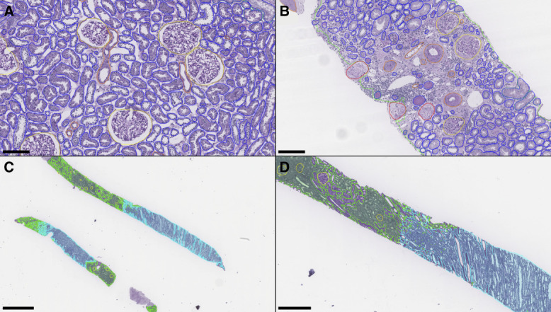
Panoptic segmentation of test set kidney biopsies. (A) Instance predictions in a kidney biopsy showing healthy/normal parenchyma. (B) Instance predictions in a kidney biopsy from a patient with creatinine >2 mg/dl. (C) Low-resolution demonstration of corticomedullary semantic segmentations. (D) Zoomed inset from the top core in (C). Green: cortex; cyan: medulla; yellow: viable glomerulus; red: sclerotic glomerulus; blue: tubule; orange: artery/arteriole. Scale bars: (A) 150 µm; (B) 150 µm; (C) 1.5 mm; (D) 500 µm.

Table 3.

Instance error rates on the test set

Class	Predicted	Partial	Missed	Fused	False Class	Total Errors
Viable glomeruli	259	0 (0%)	0 (0%)	0 (0%)	0 (0%)	0 (0%)
Sclerotic glomeruli	15	0 (0%)	1 (6.3%)	0 (0%)	0 (0%)	1 (6.3%)
Tubules	16,710	45 (0.27%)	86 (0.51%)	171 (1.02%)	7 (0.04%)	309 (1.8%)
Arteries/arterioles	552	1 (0.18%)	22 (3.83%)	2 (0.36%)	4 (0.72%)	29 (5.0%)

Values reported as absolute count (%).

For the viable glomerulus class, the network identified every glomerulus while making no false detections. The network also performed well on tubule segmentation with a 1.8% total error rate. Most tubule segmentation errors were due to the fusion of tubular boundaries, which occurred when two or more tubules were in very close proximity, often showing essentially no appreciable intervening interstitium (Figure 2A). An appreciable minority of tubule segmentation errors were missed tubules; however, these tended to be very small atrophic tubules, very small caliber tubules in the medulla, or extremely tangentially sectioned tubules (Figure 2B). Errors in the segmentation of arteries/arterioles mainly consisted of missed instances, typically of very small vessels that were bordering on the size of capillaries (Figure 2C).

Figure 2.

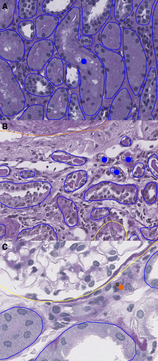
Network errors. Dots indicate missed structure. (A) Network fusion of tubular boundaries when basement membranes abut and morphologies are grossly dissimilar. (B) Network misses on small atrophic tubules. (C) Network miss on small arteriole bordering capillary size. Blue: tubule; orange: artery/arterioles.

The network was least performant in detecting sclerotic glomeruli, although the error rate is misleading because only one sclerotic glomerulus was missed of a total 16 present in the ten test cases. The one missed instance was a sclerotic glomerulus cut in half at the biopsy edge.

After the detection of erroneous instances, their boundaries were manually corrected to measure a pixel-by-pixel performance of the segmentation output. These values are reported in Table 4 and essentially reflect the instance error rate results.

Table 4.

Pixel-wise performance metrics compared against renal pathologist

Class	Sensitivity	Specificity	Precision	NPV	MCC	Dice
Glomeruli	0.998	1	1	1	0.999	0.999
Sclerotic glomeruli	0.948	1	0.996	1	0.972	0.972
Tubules	0.995	1	0.999	1	0.997	0.997
Arteries/arterioles	0.984	1	0.994	1	0.989	0.989

Dice: dice coefficient (F1 score); MCC, Matthew's correlation coefficient; NPV, negative predictive value.

As compared with previous renal pathology segmentation studies, our network outperforms other methods across all classes. These comparisons are shown in Supplemental Table 2.^8–10 Examples of additional holdout segmentations in H&E, trichrome, and silver biopsies are shown in Supplemental Figures 2, 3, and 4, respectively.

Reference Kidney Morphometrics

Using the panoptic segmentation model, measurement of histomorphometric parameters was performed for a set of reference kidneys. Because kidney tissue from individuals with no kidney disease is typically not available, this study was performed on sections of renal parenchyma uninvolved and away from the renal tumor of human tumor nephrectomy specimens. Inclusion and exclusion criteria of the reference kidney are detailed in section Reference Kidney Data and were designed to minimize the presence of abnormal histologic findings. In total, 79 multinational nephrectomy cases were included, derived from three international institutions, and each kidney section was stained with PAS. Quantified features for the reference kidney cases are tabulated in Table 1. Examples of whole-slide segmentation for reference kidneys are shown in Figure 3.

Figure 3.

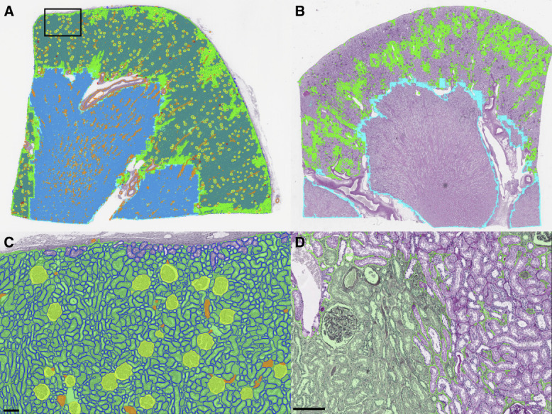
Whole-section segmentations for PAS-stained kidney nephrectomies. (A) Thumbnail of whole-segmentation mask for a reference kidney. Tubules are rendered in the background to prevent them from overwhelming the visibility of other structures. (B) Thumbnail of patchy interstitial segmentation in a kidney with many tubules flush back to back. (C) Zoomed region from (A) showing segmentation of viable glomeruli, tubules, arterioles, and cortical interstitium. (D) Zoomed region from B showing interstitium at left fused by contour retrieval after tile stitching process, where interstitium at right is patchy due to flushly abutting tubules. Green: cortical interstitium; cyan: medullary interstitium; yellow: viable glomerulus; red: sclerotic glomerulus; blue: tubule; and orange: artery/arteriole. Scale bar, 150 µm. PAS, periodic acid–Schiff.

All three institutional patient cohorts displayed similar proportions of male patients versus female patients and age distributions. SCr values, albeit varied between the institutions, were measured to be in normal range. For the histomorphometric parameters, the vast majority were similar between institutions, with a few notable exceptions as we discuss below.

For glomeruli, the average number of glomeruli per mm² of cortical tissue was 2.5, of which the average number of sclerotic glomeruli per mm² was 0.2. These values equate to a glomerulosclerosis rate of 7.3%, which matches expectations for an age range of 50–60 years. Glomerular area and radius ranged between approximately 18,800 and 23,800 µm² and 64 and 72 µm, respectively. Of note, the glomerular density varied slightly when comparing institutions in a pattern that was inversely proportional to the measured average glomerular size.

For tubules, the average number per cortical mm² also varied significantly across institutions, ranging from approximately 130 to approximately 190, again being inversely proportional with the measured average tubule size. The average area and radii of tubules ranged from 2476 to 4219 µm² and 17.92 to 23.43 µm, respectively.

Similarly, the number of observed arteries and arterioles per mm² ranged from 4 to 6 and is found to be inversely proportional with average glomerular size. That is, kidneys with larger glomeruli have lower densities of arteries and arterioles. However, we also found those arteries and arterioles to have proportionally much wider lumens because the ratio of luminal width to overall vessel width was higher, namely 0.37 as quantified for institution 2 versus 0.23 and 0.27 for institution 1 and 3, respectively.

Histomorphometric Variation across Patient Demography, SCr, and eGFR

We next used a series of adjusted linear regressions to determine whether histomorphometric measurements made on our reference kidney cohort were associated with basic patient information. This part of the study incorporated patient age, sex, and either SCr or eGFR as input variables, morphometric measurements as output values, and institutional data source as fixed effects. Table 2 summarizes model parameters for this regression analysis.

Several kidney histomorphometric parameters, especially those related to glomerular and tubular size as well as glomerular density, were significantly associated with SCr. For instance, patients with lower SCr (presumably better renal function) tended to have smaller glomeruli (i.e., smaller glomerular area and radii) but higher numbers of glomeruli per renal cortical area (i.e., high glomerular density). Similarly, tubular radii were larger in patients with higher SCr levels. Interestingly, when looking at the SD for the distribution of glomerular and tubular sizes within a kidney tissue section, glomerular size distribution varied less when patients had high SCr levels, while tubular size distribution varied more with higher SCr levels.

In addition, several kidney histomorphometric parameters were associated with patient eGFR. Most of the same histomorphometric parameters that were associated with SCr were also associated with eGFR, but with an inverse in the magnitude of the associations. For instance, patients with higher eGFR tended to have smaller glomeruli and higher numbers of glomeruli per cortical area. The same trend was apparent in the tubular radius. This is to be expected because higher SCr measurements directly lead to a lower calculation of eGFR.

Fewer significant associations were seen for patient sex and age. The glomerulosclerosis ratio (essentially the percentage of glomerulosclerosis) and the density of arteries/arterioles were significantly higher for men than women. In addition, the SD for the glomerular area of any given patient tended to be higher for men than women. Regarding age, one of the only parameters that showed significant association was cortical arterial/arteriolar area density, which was positively correlated to age, meaning that with an increase in age, the total area of arteries and arterioles occupying a given amount of cortex increases. The percentage of glomerulosclerosis also showed a positive trend with age.

The distribution of histomorphometric parameters within each patient's kidney tissue section was also examined using kernel density estimations coded by color reflecting the patient's SCr (Figure 4). As illustrated in Figure 4A, the average and spread (i.e., SD) of cortical tubular radii were both higher in patients with higher SCr values. Similarly, the average glomerular radii (Figure 4B) were higher in patients with higher SCr, but the SDs were slightly lower in patients with higher SCr. This observation suggests that as glomeruli hypertrophy compensates for increased creatinine, they may reach an expansion limit of approximately 100 µm in radius. Interestingly, the average sclerotic glomerulus radius was also dependent on creatinine.

Figure 4.

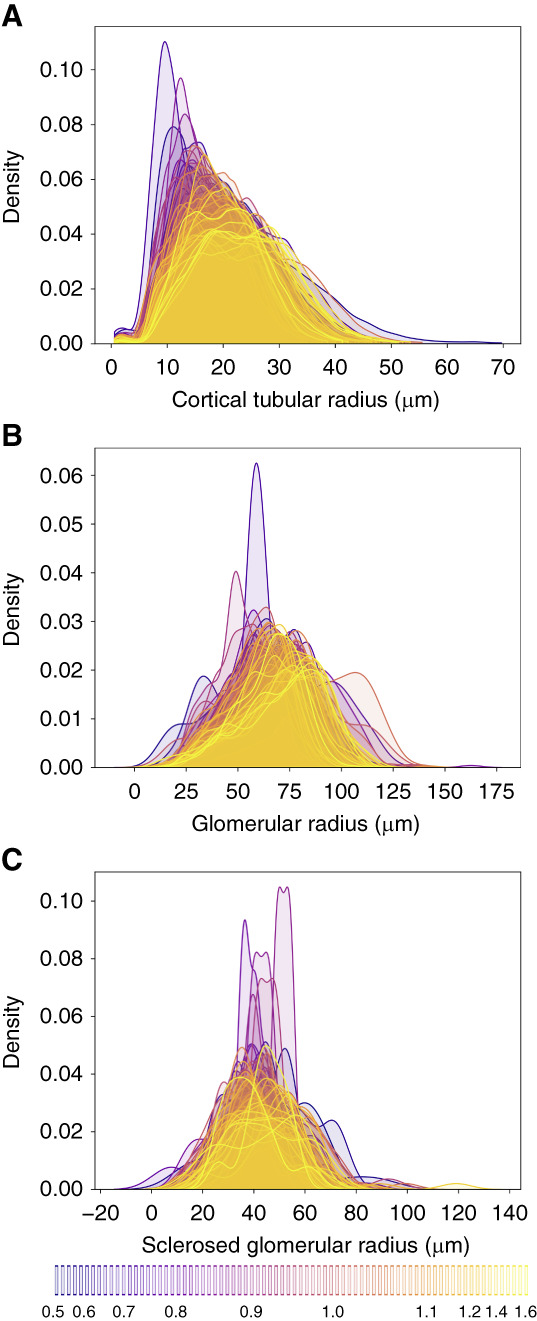
Probability density estimates for glomerular and tubular radii per patient. Color is coded by creatinine with the lowest values in blue and the highest values in yellow as indicated by the bottom legend. (A) Radii of cortical tubules. (B) Radii of viable glomeruli. (C) Radii of sclerosed glomerular.

Discussion

Image segmentation allows for the detection and classification of histologic structures and is considered a foundational step in the development of computational pathology and an absolute requirement for automated histomorphometric analysis. Generally, segmentation methods can be classified as either semantic segmentation or instance segmentation. In semantic segmentation, a classification label is assigned to every pixel in the image, but this method is limited in that it cannot distinctly recognize two same-class entities that are abutting or overlapping. By contrast, instance segmentation is the task of distinctly recognizing abutting/overlapping objects as unique entities. However, such algorithms are typically unable to model multiple classes. Numerous studies have shown the undeniable utility of deep neural networks for segmentation tasks in digital pathology datasets. Yet, most prior networks were constrained either for semantic segmentation or instance segmentation alone, unable to leverage the strengths of each method in combination. More recently, the development and maturation of panoptic architectures has led to the ability to segment both semantic and instance objects simultaneously, allowing for a comprehensive approach to histomorphometric image analysis. In this work, we demonstrate the feasibility of using a panoptic segmentation neural network–based pipeline to accurately quantify a variety of histomorphometric parameters from WSIs of reference kidney tissue sections. The high segmentation performance of our model allowed us to take the first steps in defining reference morphometrics for healthy human kidneys on over three million nephrons.

Although a large amount of histomorphometric data can be extracted using our automated DL-based image analysis pipeline, the measurements are only useful if they have some type of biological or clinical relevance. Thus, we subsequently used simple regression analysis to identify relationships between histomorphometric parameters of healthy kidneys to patient age, sex, SCr, and eGFR. Several histomorphometric parameters that reflect glomerular and tubular size and glomerular density significantly associated with patient SCr levels. Our observations are consistent with previous studies, which indicate that glomerular and tubular size tends to be directly associated with SCr levels, while glomerular density (as estimated by the number of glomeruli per renal cortical area) is typically inversely associated with SCr levels.

Previous studies quantified reference kidney morphometrics in both a manual and automated fashion. As compared with previous works, our study involves a larger and more diverse sample set and leverages computational methods to improve scalability. Samuel et al.¹¹ investigated 24 kidney samples, with 12 coming from patients aged 20–30 years and 12 coming from patients aged 51–69 years. These patients were previously reported as healthy, but they died unexpectedly from nonrenal causes. Glomerular number and glomerular volume were measured using the dissector/Cavalieri method.¹² To extend our glomerular area measurements to volume, we used the Weibel–Gomez method.¹³ Glomeruli were assumed to be spherical, using 1.38 as the shape coefficient and 1.01 as the size distribution coefficient, assuming a 10% variation in glomerular volume, similar to previous studies.¹⁴ A comparison with the study of Samuel et al. is shown in Supplemental Table 3A. Our average estimates for glomerular volume are smaller than previously reported, which may be attributable to differences in measurement techniques. Estimations of three-dimensional volumes from a single 2-dimensional cross-section are likely less accurate than the dissector/Cavalieri method, which uses multiple cross-sections to estimate volume. However, as compared with the cohort of patients aged 51–69 years, which more accurately reflects the age range of our cohort, a two-sample Student's t test proved the measurements of percentage glomerulosclerosis are not significantly different.

In the study of Hölscher et al., computational methods were also used to analyze renal WSIs and report morphometrics.¹⁰ These measurements were reported from 17 samples from an internal biopsy cohort from the Institute of Pathology in Aachen that were classified as histologically normal. Glomeruli and tubules, along with other renal structures, were segmented through a DL pipeline and quantified from their associated segmentation masks. These results are reported as median and interquartile range in Supplemental Table 3B. Our results are similar to those reported in the previous study. The relative similarity is to be expected because reference samples are being quantified in a similar manner. Most other features quantified in this study are not comparable with previous studies.

Our study has a few major limitations. First is the definition and use of reference kidneys. Depending on the stringency of defining the criteria for reference kidney samples, true reference kidney samples are difficult to obtain given the ethical considerations. One alternative would be using autopsy kidneys; however, these samples typically have prominent degradation/decomposition artifact, which would likely confound histomorphometric analysis. In our study, we used kidney parenchyma from tumor nephrectomy specimens distanced from the tumor foci and screened for minimal abnormalities by a pathologist. Such specimens are likely the most readily available, although the age of the patients is skewed to older individuals. In addition, analysis of a tumor that could potentially result in a mass effect–related issue like obstruction could confound the data even after a pathologist has screened for normal-appearing sections. Another limitation is that we used large tissue sections from nephrectomy specimens that may not easily translate to equivalent histomorphometric values seen on biopsy. Typical biopsies have a much smaller surface area, which results in significantly lower numbers of glomeruli, tubules, and vessels, as well as a high proportion of transected structures at the edge of the biopsy. Whether reference kidney histomorphometric values need to be re-established in smaller biopsy specimens to be useful in the clinical setting needs to be evaluated. Furthermore, we used specimens from three different institutions, which likely resulted in an institutional-specific batch effect. Further evaluation to examine in detail the histomorphometric effects of processing tissue at different institutions must be determined.

To our knowledge, our work is the most comprehensive study to tabulate large-scale reference renal morphometry features with clinical significance using a large, diverse, multinational, highly quality controlled cohort of renal tissue biopsy images. Ultimately, reference kidney histomorphometric values require examination of a large cohort from various populations, which will likely be achievable by upscaling our current strategy. Such data would allow eventual quantitative or statistical definitions for certain types of pathologic entities. For instance, tubular atrophy could 1 day be defined as tubules with radii below a certain statistical threshold. Similarly, defining glomerulomegaly may be more straightforward, and diagnosis may be aided by automated morphometry.

Disclosures

B. Ginley reports the following—Employer: Johnson & Johnson and SUNY Buffalo. S.S. Han reports the following—Research Funding: Daewoong Pharmaceutical. S. Jain reports the following—Patents or Royalties: AMIRYSIS Inc. and Elsevier; Advisory or Leadership Role: HUBMAP and KPMP; and Other Interests or Relationships: Amirsys Inc., CZI Human Cell Atlas Project workshop, Duke University (speaker), FASEB-AKI annual workshop, Nanostring research collaboration, NKF southwest chapter, Royalty for book chapters in Diagnostic pathology: Kidney Diseases, SenNet consortium (speaker), and University of Virginia (speaker). K.-Y. Jen reports the following—Advisory or Leadership Role: Novartis; and Speakers Bureau: Alexion. G. Nadkarni reports the following—Consultancy: Daiichi Sankyo, GLG consulting, Qiming Capital, Reata, Renalytix, Siemens Healthineers, and Variant Bio; Ownership Interest: Data2Wisdom LLC, Doximity, Nexus iConnect, Pensieve Health, Renalytix, and Verici; Research Funding: Renalytix; Honoraria: Daiichi Sankyo; Patents or Royalties: Renalytix; Advisory or Leadership Role: Renalytix; and Speakers Bureau: Daiichi Sankyo. J. Zee reports the following—Honoraria: Booz Allen Hamilton. All remaining authors have nothing to disclose.

Funding

P. Sarder's work is supported by NIH-NIDDK grant R01 DK114485, R01 DK131189, R21 DK128668, via the opportunity pool funding mechanism, namely via the glue grant mechanism of the NIH-NIDDK Kidney Precision Medicine Project (KPMP) consortium grant U2C DK114886, via the KPMP Kidney Mapping and Atlas Project (KMAP) U01 DK133090, NIH-OD Human Biomolecular Atlas Project (HuBMAP) consortium Integration, Visualization and Engagement (HIVE) project OT2 OD033753, NIH/NCI Coordinating and Data Management Center for Acquired Resistance to Therapy Network U24 CA274159, and faculty start-up funding from University of Florida.

Author Contributions

Conceptualization: Kuang-Yu Jen, Pinaki Sarder.

Data curation: Brandon Ginley, Seung Seok Han, Sanjay Jain, Kuang-Yu Jen, Luis Rodrigues, Pinaki Sarder, Michelle L. Wong.

Formal analysis: Brandon Ginley, Nicholas Lucarelli, Pinaki Sarder, Jarcy Zee.

Investigation: William L. Clapp, Brandon Ginley, Seung Seok Han, Sanjay Jain, Kuang-Yu Jen, Nicholas Lucarelli, Girish Nadkarni, Tezcan Ozrazgat-Baslanti, Luis Rodrigues, Pinaki Sarder, Michelle L. Wong, Jarcy Zee.

Methodology: Brandon Ginley, Kuang-Yu Jen, Pinaki Sarder, Jarcy Zee.

Resources: Seung Seok Han, Sanjay Jain, Kuang-Yu Jen, Luis Rodrigues, Pinaki Sarder.

Software: Sayat Mimar, Anindya S. Paul.

Supervision: Pinaki Sarder.

Validation: Sayat Mimar, Tezcan Ozrazgat-Baslanti, Anindya S. Paul.

Visualization: Sayat Mimar, Anindya S. Paul.

Writing – original draft: Nicholas Lucarelli and Brandon Ginley.

Writing – review & editing: William L. Clapp, Seung Seok Han, Sanjay Jain, Kuang-Yu Jen, Nicholas Lucarelli, Sayat Mimar, Girish Nadkarni, Tezcan Ozrazgat-Baslanti, Anindya S. Paul, Luis Rodrigues, Pinaki Sarder, Michelle L. Wong, Jarcy Zee.

Data Sharing Statement

Partial restrictions to the data and/or materials apply. All 79 reference whole slide images (WSIs) and segmented renal microcompartments are available for viewing using Digital Slide Archive (DSA),⁷ a tool for archiving and large-scale scalable visualization of gigapixel size WSIs, and also for developing plugins for conducting computational assessment of WSIs, at https://athena.rc.ufl.edu, under Collections/Journals/reference_slides_brightfield_histology_lucarelli_kidney360_2023. See more details on how to navigate the WSIs with computational annotations in the Supplemental Materia; particularly in Supplemental Figures 5-8. Clinical metadata associated with these slides are also made available from the same location in DSA. The segmentation algorithm used in this study has been implemented as a plug-in to the slide viewer and is publicly available for users to upload, segment, and quantify their PAS-stained kidney WSIs. After opening the image in HistomicsUI, the MultiCompartmentSegment plugin is chosen under sarderlab/ComPRePS/segmentation with the pretrained model to predict on WSI. The code, along with instructions to run the plug-in at DSA, is available at https://github.com/SarderLab/Multi-Compartment-Segmentation. Instructions for computing the morphometric features from segmented compartments that we quantified in this work are available in the github repository, https://github.com/SarderLab/Summary_Feature_Extraction. Feature extraction can also be conducted using a dedicated plugin that we implemented in our DSA portal at https://athena.rc.ufl.edu.

Supplemental Material

This article contains the following supplemental material online at http://links.lww.com/KN9/A406.

Augmentation Strategy.

Supplemental Table 1. Full list of tested morphometrics and reference values (N=79 participants, one whole-slide image per participant).

Supplemental Table 2A. Segmentation accuracy comparison with previous study.

Supplemental Table 2B. Segmentation dice coefficient comparison with previous studies.

Supplemental Table 3A. Feature measurement comparison with previous study.

Supplemental Table 3B. Feature measurement comparison with previous study.

Supplemental Figure 1. Examples of distance transform applied to various tubular segments.

Supplemental Figure 2. Holdout segmentation of H&E biopsy after inclusion of 23 small training regions totaling 34 mm².

Supplemental Figure 3. Holdout segmentation of trichrome biopsy after inclusion of four annotated trichrome training patches totaling only 1.4 mm² of tissue.

Supplemental Figure 4. Holdout segmentation of silver biopsy after inclusion of two annotated silver training patches totaling only 2 mm² of tissue.

Supplemental Figure 5. Digital slide archive (DSA).

Supplemental Figure 6. Digital slide archive (Cont.).

References

- 1.Inker LA Eneanya ND Coresh J, et al.; Chronic Kidney Disease Epidemiology Collaboration. New creatinine- and cystatin C-based equations to estimate GFR without race. N Engl J Med. 2021;385(19):1737–1749. doi: 10.1056/NEJMoa2102953 [DOI] [PMC free article] [PubMed] [Google Scholar]
- 2.Kirillov A, Girshick R, He KM, Dollar P. Panoptic feature pyramid networks. 2019 IEEE/CVF Conference on Computer Vision and Pattern Recognition (CVPR) 2019:6392–6401. doi: 10.1109/Cvpr.2019.00656 [DOI] [Google Scholar]
- 3.Merz G Liu Y Burke CJ, et al. Detection, instance segmentation, and classification for astronomical surveys with deep learning (DEEPDISC): DETECTRON2 implementation and demonstration with Hyper Suprime-Cam data. Monthly Notices of the Royal Astronomical Society. 2024;526(1):1122–1137. doi: 10.1093/mnras/stad2785 [DOI] [Google Scholar]
- 4.Kreyszig E. Advanced Engineering Mathematics. In: Access Pack E-Text Card, 10th ed. John Wiley & Sons; 2015. [Google Scholar]
- 5.Armstrong RA. When to use the Bonferroni correction. Ophthalmic Physiol Opt. 2014;34(5):502–508. doi: 10.1111/opo.12131 [DOI] [PubMed] [Google Scholar]
- 6.Mackinnon JG, White H. Some heteroskedasticity-consistent covariance-matrix estimators with improved finite-sample properties. J Econom. 1985;29(3):305–325. doi: 10.1016/0304-4076(85)90158-7 [DOI] [Google Scholar]
- 7.Gutman DA Khalilia M Lee S, et al. The digital slide archive: a software platform for management, integration, and analysis of histology for cancer research. Cancer Res. 2017;77(21):e75–e78. doi: 10.1158/0008-5472.CAN-17-0629 [DOI] [PMC free article] [PubMed] [Google Scholar]
- 8.de Bel T, Hermsen M, Smeets B, Hilbrands L, van der Laak J, Litjens G. Automatic Segmentation of Histopathological Slides of Renal Tissue Using Deep Learning. SPIE; 2018. [Google Scholar]
- 9.Bouteldja N Klinkhammer BM Bülow RD, et al. Deep learning-based segmentation and quantification in experimental kidney histopathology. J Am Soc Nephrol. 2021;32(1):52–68. doi: 10.1681/ASN.2020050597 [DOI] [PMC free article] [PubMed] [Google Scholar]
- 10.Hölscher DL Bouteldja N Joodaki M, et al. Next-generation morphometry for pathomics-data mining in histopathology. Nat Commun. 2023;14(1):470. doi: 10.1038/s41467-023-36173-0 [DOI] [PMC free article] [PubMed] [Google Scholar]
- 11.Samuel T, Hoy WE, Douglas-Denton R, Hughson MD, Bertram JF. Determinants of glomerular volume in different cortical zones of the human kidney. J Am Soc Nephrol. 2005;16(10):3102–3109. doi: 10.1681/ASN.2005010123 [DOI] [PubMed] [Google Scholar]
- 12.Roberts N, Cruz-Orive LM, Reid NM, Brodie DA, Bourne M, Edwards RH. Unbiased estimation of human body composition by the Cavalieri method using magnetic resonance imaging. J Microsc. 1993;171(Pt 3):239–253. doi: 10.1111/j.1365-2818.1993.tb03381.x [DOI] [PubMed] [Google Scholar]
- 13.Weibel ER, Gomez DM. A principle for counting tissue structures on random sections. J Appl Physiol. 1962;17(2):343–348. doi: 10.1152/jappl.1962.17.2.343 [DOI] [PubMed] [Google Scholar]
- 14.Nielsen CM Skov K Buus NH, et al. Kidney structural characteristics based on a kidney biopsy and contrast-enhanced computed tomography in healthy living kidney donors. Anat Rec (Hoboken). 2020;303(10):2693–2701. doi: 10.1002/ar.24359 [DOI] [PubMed] [Google Scholar]
Associated Data
This section collects any data citations, data availability statements, or supplementary materials included in this article.
Supplementary Materials
Data Availability Statement