Demand charges reduction with photovoltaics in industry

Abstract

Demand charges are widely used for commercial and industrial consumers. These costs are often not well known, let alone the effects that PV can have on them. This work proposes a methodology to assess the effect of PV on reducing these charges and to optimise the power to be contracted, using techniques taken from exploratory data analysis. This methodology is applied to five case studies of industrial consumers from different sectors in Spain, finding savings between 5 % and 11 % of demand charges in industries with continuous operation and up to 28 % in cases of discontinuous operation. These savings can be even greater if the maximum power that can be contracted is lower than the optimum. The demand charges in Spain consist of a fixed part proportional to the contracted power and a variable part depending on the power peaks exceeding it. Since for the variable part the coincident and non-coincident models coexist, a comparison is made between the two models, finding that in the general case PV users can achieve higher savings with the coincident model.

Graphical abstract

Highlights

• •A methodology for analysis of peak load is proposed.
• •An algorithm for optimizing contracted power is developed.
• •A reduction in PV demand charges of up to 13 % has been observed for the general case.
• •PV savings in demand charges are higher for the coincident scheme.
• •Coincident demand charges prove more beneficial for all stakeholders.

Nomenclature

$F_{EP}$

Demand charges (monthly)

$t_p$

Cost of non-coincident demand charges in €/kW

$P{c}_P$

Contracted power in period P

$P{d}_P$

Maximum demanded power in each one of the periods exceeding $P{c}_P$

$K_p$

Ratio of the toll for each period p to the toll for period 1

$t_{ep}$

Demand charge coefficient

${Pd}_j$

$j^{th}$ 15-min average power exceeding contracted power

Abbreviations

DER

Distributed Energy Resources

DSO

Distribution System Operator

EDA

Exploratory Data Analysis

LCOE

Levelized Cost of Energy

PV

Photovoltaic

TOU

Time of Use

TROI

Time of Return on Investment

TSO

Transmission System Operator

1. Introduction

The decreasing costs of distributed energy sources, in particular PV, have led to a significant increase in the number of consumers becoming prosumers; in addition to this fact, there are new obligations for large and small and medium-sized companies which may provide an additional boost as the new European Sustainability Directive [1] will obligate them to report on the implementation of sustainability issues in business. This includes information needed to understand the sustainability impacts of companies, and how sustainability issues affect the development, performance, and position of companies.

Following the transformation of many grid users from passive to active agents may lead to an imbalance in the financing of the fixed costs of the electricity grid. Frequently, current grid price structures do not provide enough grid cost recovery and lack the incentive to promote effective grid investment [2]. In this way, there are growing concerns about the avoided costs by the DER adopters that could result in wealth transfers between consumers [3]. One of the mechanisms frequently considered to compensate the decline in fixed costs recovery are demand charges [4]. Unlike energy charges, which hinge on electricity usage, demand charges consider peak power consumption during specific time intervals. These charges aim to mirror the strain imposed on the grid during high-demand periods and motivate consumers to optimise their peak energy consumption. As electricity generation and the grid must meet peak demand, the most equitable way to share these costs between consumers is generally considered to be through demand charges as DER adopters can avoid a significant part of energy consumption but reduce peak demand very little.

Demand charges can be implemented in a variety of ways [5]. In many cases the most basic model is used, which is the non-coincident model. In this case the payment is determined by the customer's peak demand during the month, regardless of the time of day. This model is simple to understand for consumers but poses problems, the most obvious being that a consumer whose peak demand coincides with the system's peak demand pays the same as a consumer whose peak occurs at off-peak times and therefore does not place any stress on the grid [6], or that a consumer with a sporadic peak might pay more than consumers with recurring peaks. Many economists prefer a TOU tariff to avoid these shortcomings [7], and note than TOU can provide better welfare gains than demand charges [8]. Other designs of demand charges try to avoid these shortcomings by introducing hourly and/or seasonal windows coinciding with system peaks. Coincident demand charges are therefore more expensive during peak hours and months. In addition, demand charges may also include a fixed term that is paid even if the peak demand is lower than the contracted power or a fixed percentage of the peak demand in the previous 12 months (ratchet) [9]. Coincident demand charges applied when network peaks are likely to occur are considered to be more reflective [10].

Commercial and industrial consumers are subject to demand charges in most countries, although these charges are often not well known. The research in Ref. [11] points out that cost analyses rarely consider the effects of demand charges, that can exceed costs for energy use in some industries and are relevant for choices like shift-schedules, process design, or investing in self-generation and/or energy storage. Once the importance of demand charges has been recognized, the issue for consumers is to optimise electricity contracts to minimize the cost of demand charges in the electricity tariff. A framework for optimisation of demand in Brazil is proposed in Ref. [12] and the possibility of savings of more than 40 % is reported for irregular load profiles. This framework is based on a graphical method using the monthly maximum demand for the previous year and assuming a linear model for the demand profile.

Due to the growing proportion of prosumers, the introduction of demand charges for residential consumers is increasingly being considered. However, the difficulty in justifying their necessity and their complex operation is holding back their implementation, with few countries and/or utilities offering or being mandatory for residential customers. The case of demand charges adoption in residential consumers has been widely reported in the literature both at the tariff design level [13] and with cases of study. For example, in Ref. [14] demand charges are analysed through an optimisation problem, which is solved with a genetic algorithm for optimal battery sizing and annual energy cost under time of use and demand charges billing schemes.

Solar PV can reduce peak load consumption, as it is shown in Fig. 1, but the availability of the solar resource limits the potential of demand charges reductions, which can be further reduced through the use of batteries. In spite of industrial facilities accounting for 42 % of the world's total delivered electricity [15] and that usually are subjected to demand charges, few studies have been dedicated to the effect of PV on demand charges in industry. A SCOPUS search with the keywords “demand charges” AND “PV” AND “Industrial” in the fields of title, abstract and keywords result in only 15 journal and conference papers published between 2010 and 2022. Demand charge savings from PV where studied in Ref. [16] in a case study of an university campus concluding that PV often provide very small demand reductions. The complementary addition of batteries to PV to further reduce demand charges is studied in Ref. [17]. In this work, typical load profiles of nine commercial and industrial end-users were used for the design of the PV and battery combination, and the optimisation of battery capacity and PV load to minimize demand loads was performed using sensitivity analysis. A review on maximum demand shaving with application to the Malaysian electricity tariff is presented in Ref. [18], finding a good return on PV-battery investment for commercial and industrial customers. A novel self-adjusting controller of battery storage in a university building achieve a maximum demand reduction of 11 % for a 18 kW/99 kWh battery and 11 kW PV [19]. The importance of retail rate design for PV and battery storage in commercial and industrial prosumers is studied in Ref. [20], and it is found that retail tariffs with high demand charges and low volumetric TOU rates are more effective motivating storage investment but reduce incentives to invest in PV. The high demand for batteries is causing battery prices not to decrease in a similar way to PV systems. It is therefore necessary to have a thorough understanding of the reduction in demand charges due to PV. The academic research is mainly focused on battery storage, which complements PV in demand charge reductions. However, little research has been done on quantifying the reduction in demand charges due to PV only. The main objective of the present work is to develop a methodology to quantify the reduction in peak load due to the incorporation of PV with application to demand charges optimisation in industrial PV adopters. In the case of Spain and other countries, demand-side tariffs are set according to peak consumption in 15-min intervals, which makes the accuracy of electricity demand forecasting methods and solar production difficult. This is why the proposed method is based on the historical series of the preceding year. Using a full year's quarter-hourly data set for five case studies, the research has been developed and cross-checked with electricity bills from one of them.

Fig. 1.

Peak load reduction with photovoltaic self-consumption system.

The main contributions of this work are as follows.

• •A methodology for analysis and optimisation of demand charges optimisation. It is applied under the current regulation in Spain, where demand charges consist of a fixed part depending on the contracted maximal power and a variable part depending on the maximum power exceeding the contracted one during the billing period. The optimisation determines the optimal maximal power to be contracted to minimize demand charges considering the effect of PV in reducing the amount of excess power.
• •The verification of the feasibility of demand charge reduction in the electricity bills of industrial buildings through the utilisation of solar PV by means of five study cases representative of different industries.
• •The present research distinguishes itself from prior analyses by comparing the efficiency of coincident and non-coincident demand charges, thereby imparting wider relevance due to the paucity of experimental studies on this subject beyond local contexts.

The paper is organized as follows: Section 2 presents the Spanish regulation on demand charges for commercial and industrial customers, where both coincident and non-coincident models co-exist. Section 3 presents the methodological framework used to identify and classify the peak load registered in the year of operation used for the calculation of demand charges in this investigation. It also sets out the algorithm used to establish the optimal powers to be contracted. The main results of this study are presented in Section 4. These results are discussed in Section 5 and the conclusions are summarized in Section 6.

2. Demand charges regulation in Spain

Currently, in Spain there are three electricity pricing groups under a time of use (TOU) scheme [21]. In low voltage (less than 1 kV), there are the 2.0TD rate for contracted power lesser than 15 kW, mainly for domestic users and small businesses, and the 3.0TD for commercial, administrative, and small industries. In high voltage there are the so called 6.xTD tariffs, (x correspond to the voltage level) in use in large commercial, administrative and industrial sectors. For the 3.0TD and 6.xTD tariffs, six pricing periods are defined, which are shown in Fig. 2, being P1 the highest priced and P6 the lowest. The contracted power can be different for each of the six periods, but with the limitation that it must be increasing from P1 to P6. The daily periods are set in three categories: “peak”, “flat” and “valley”, correlated with the national grid load. Depending on the season (high, high-mid, mid, low), different pairs of periods are assigned to the peak and flat categories: P1–P2, P2–P3, P3-4, P4–P5, while the valley hours are always P6.

Fig. 2.

Pricing periods for tariffs 3.0TD and 6.xTD in Spain. Weekends and public holidays are P6.

The electricity bill in Spain is made up of several sections: contracted power term, energy term, penalties for excess power, penalties for reactive power, and taxes. Demand charges are implemented as the sum of a fixed charge (contracted power term that increases linearly with contracted power in $€/kW/year$) plus a variable charge (penalties in case of exceeding the contracted power). The energy consumption term may have fixed energy prices for each period or may be indexed to the wholesale electricity price (spot price plus TSO technical costs, regulated charges and tolls, and commercial margin). The charges and tolls differ for each period, being higher for P1 and lower for P6. As previously indicated, penalties for excess power (variable demand charges) are applied when more power than that contracted is demanded. The record of the monthly maximum demanded power depends on the type of electricity meter available at the consumer's site. As a rule, for contracted power lower than 50 kW the peak demanded power is metered by means of a maximeter, which averages the power demanded in 15-min intervals and records the monthly maximum in each period from P1 to P6, following a non-coinciding scheme. For contracted power higher than 50 kW the electricity meter records the average power in every quarter of an hour and the data is sent to the distribution system operator (DSO) to calculate the penalties in a coincident scheme.

For contracted powers below 50 kW, demand charges are non-coincident and apply in the event that the maximum power demanded exceeds 105 % of the contracted power for each pricing period. These charges are calculated according to Eq. (1).

$$F_{EP}=\sum _{P=1}^{P=i}{t}_p\bullet 2\bullet \left(P{d}_P-1.05\bullet P{c}_P\right)$$ (1)

Where:

$F_{EP}$: Demand charges (monthly)

$t_p$: Cost in €/kW. For tariff 3.0TD and year 2023 it is of 0.112 €/(kW day)

$P{d}_P$: Maximum demanded power in each one of the periods exceeding $P{c}_P$.

$P{c}_P$: Contracted power in period P.In the defunct tariff 3.1A, applicable for consumers connected to the high-voltage public grid with contracted power up to 450 kW, demand charges followed this method but the power terms tariff for the periods P1–P3 were used instead of the $t_p$ coefficient. That method charged the power excesses with the double of the difference between the maximum demanded power and the contracted power. That method was very expensive and in the new tariffs the coefficient $t_p$ is the same for all periods, resulting in a non-coincident demand charge. These demand charges are applied regardless of the number of times the contracted power has been exceeded in the corresponding period and therefore favours users with frequent excesses over users with sporadic ones.

For contracted powers over 50 kW, the demand charges follow a coincident model and are calculated according to the expression of Eq. (2)

$$F_{EP}=\sum _{\mathrm{P}=1}^{\mathrm{P}=\mathrm{i}}{K}_p\bullet {\mathrm{t}}_{\text{ep}}\bullet \sqrt{\sum _{j=1}^n{\left({Pd}_j-P{c}_P\right)}^2}$$ (2)

Where.

• $K_p$: Ratio of the toll for each period p to the toll for period 1. Values are given in Table 1.

• ${\mathrm{t}}_{\text{ep}}$: Demand charge coefficient for each period. It is established annually and takes value of 3.66 for year 2023 (Table 2), showing a great increase from 2021.

• ${Pd}_j$: $j^{th}$ 15-min average power exceeding contracted power.

• $\mathrm{P}{\mathrm{c}}_{\mathrm{P}}$: Contracted power in period P.

Table 1.

Values of $K_p$ coefficient for the year 2023.

Pricing period	P1	P2	P3	P4	P5	P6
$K_p$ 3.0TD	1	0.97	0.26	0.22	0.13	0.13
$K_p$ 6.1TD	1	0.94	0.46	0.37	0.026	0.026

Table 2.

Values of demand charge coefficient $t_{ep}$ for years 2021–2023 [[22], [23], [24]].

Tariff	3.0TD	6.1TD
$t_{ep}$ (€/kW) 2021	1.41	1.41
$t_{ep}$ (€/kW) 2022	2.47	2.50
$t_{ep}$ (€/kW) 2023	3.42	3.66

When studying the function in Eq. (2), it can be seen that the successive excesses have a smaller incidence on the penalties. Indeed, if it is assumed the hypothesis of a number n of equal excesses with maximum power $P_d$ for an arbitrary billing period $i$ and the same contracted power for all periods $P_c$ , the demand charges for the i-th period will be given according to Eq. (3). In this way, the first excesses have a greater penalty, which is gradually reduced, but the shape of the √n function makes them continue increasing. This is a fair mechanism that penalises excesses and distinguishes between different behaviours: sporadic excesses versus frequent excesses.

$$F_{Ei}=K_p\bullet {\mathrm{t}}_{\text{ep}}\bullet \sqrt{\sum _{i=1}^n{\left(Pd-P{c}_i\right)}^2}=K_p\bullet {\mathrm{t}}_{\text{ep}}\bullet \sqrt{n\bullet {\left(Pd-Pc\right)}^2}=K_p\bullet {\mathrm{t}}_{\text{ep}}\bullet \left(Pd-P{c}_i\right)\bullet \sqrt{n}$$ (3)

The coefficient values $K_p$ shows the coincident nature of this demand charge model (Table 1). In fact, for periods of higher national electricity demand (P1 and P2), this coefficient takes the maximum value of 1, but for periods of lower electricity demand (P5 and P6) the coefficient is approximately forty times lower. For the year 2022 and 2023, these coefficients have slight variations with respect to the values in 2021.

Given the importance of contracting the optimal power that results in the lowest cost of demand charges, it may be necessary to make variations in contracted power. In Spanish regulation, this change can be done at any time, but the following costs must be borne: but the following costs must be faced: access cost, which includes the bureaucratic process; extension cost, linked to the use of the infrastructure necessary for this additional power; and action cost in case the intervention of a technician is necessary [25], that are shown in Table 3. The extension costs are valid for three years. It is important to note that in a context of possible grid saturation in mature industrial areas, if the contracted power is lowered, the extension rights are lost after three years and if another customer increases its power, it may not be possible to contract more power due to grid limitations.

Table 3.

Costs for contracting different maximum power. Access costs covers the bureaucratic process, extension costs are linked to infrastructure use due to increased power and action costs are paid if a technician is required on site.

Tariff	Access costs	Extension costs	Action costs
3.0TD	19.7 €/kW	17.4 €/kW	9 €/actuation
6.1TD	17.0 €/kW	15.7 €/kW	79 €/actuation

3. Methodology

3.1. Data analysis framework

The starting point for studying excess power logically seems to be the presentation of the time series of consumed, PV produced and demanded power for a full year. However, the large amount of information presented does not allow to easily detect patterns of behaviour beyond the purely seasonal ones, as can be seen in Fig. 3(a) where the data for one of the case studies is shown. Moreover, it is difficult to determine the power to be contracted to avoid or minimize demand charges (Fig. 3(b)).

Fig. 3.

Time series for one of the study cases (#4). (a) Annual electricity consumption. (b) Time series of electricity consumption and electricity demanded from the grid for one week.

For this analysis, some concepts from Exploratory Data Analysis (EDA) [26] are used. Firstly, the daily behaviour is explored using box and whiskers plot diagrams (boxplots) [27] for the electricity consumed, PV produced and imported from the grid. As the consumption may depend on seasonal situations or on the weekly variation itself, it is useful to plot the daily consumption over the year beforehand to detect possible patterns of operation. Usually, it is only necessary to trace different boxplots for weekdays and for weekends and holidays to identify possible patterns of operation. In case there are periods with different consumption levels, it may be necessary to process the daily consumption information to identify the different situations and trace the boxplots for each. The impact of PV production on excesses is analysed by plotting heatmaps of the excesses for each day of the year against the time of day for the industrial facility with and without PV support. These graphs give qualitative information on the impact of photovoltaics, especially important for identifying clusters at different times of the year and specific hours of the day, which are closely related to the monthly billing periods (P1 to P6). This information, being qualitative, is not sufficient for an accurate assessment of the impact of photovoltaics on the excesses. A further step is taken through the use of load duration curves. These curves are widely used in power generation, especially for planning. A load duration curve is the representation of the load over the course of a year ordered from highest to lowest. In this work, load duration curves for the energy taken from the grid with and without PV will be constructed for each applicable period (P1.P6) of each month (billing period) and compared with the contracted power as a previous step for the calculation of the demand charges. This calculation is accomplished using Ec. (2) on the excesses computed using the load duration curves for every applicable period of each month, as it is outlined in the diagrams of Fig. 4(a and b), allowing to quantify the demand charges savings due to PV.

Fig. 4.

Analysis of demand charges in the case study: a) Overall data analysis; b) Method of calculation of load duration curves.

3.2. Optimisation of contracted power

Once a method of calculating excess power has been developed, the next step is to use it to calculate the demand charges for a range of contracted powers adapted to the energy consumed and the power demanded. The algorithm proposed is detailed in Fig. 5. This algorithm is applicable to both the coincident (P > 50 kW) tariff scheme and the non-coincident 3.0TD (P < 50 kW) tariff scheme. The load duration curves are calculated for each month and applicable period. For the range of contracted powers corresponding to each particular study case the load duration curves are used to determine the partial results for each month and period according to Eq. (1) or Eq. (2) depending on the scheme of demand charges. These partial results are stored in case further in-deep analysis is required. With these results, the fixed and variable part of the demand charges are calculated. Finally, with the detailed demand charges results it is possible to run the optimisation algorithm. In the present work a straightforward algorithm is enough for the power optimisation.

Fig. 5.

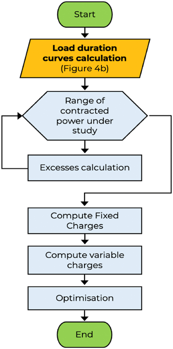
Algorithm for optimisation of contracted power.

Since the calculation of the demand charges is available for every applicable period from each month, it will be made for a range of contracted power values in all periods. Finally, power optimisation is carried out to maximize the economic savings. The basic approach is to contract equal power for all periods, but the regulation in force in Spain allows to contract different powers for each period as long as they are increasing from P1 to P6. In this way, it is possible to run a simple optimisation algorithm to find the optimal combination of contracted powers for each period.

3.3. Case studies

The case studies used in this work are representative of different production situations common in the industry in terms of electricity consumption patterns. All facilities are located in the interior of the country, as shown in Fig. 6. Industries #1 and #3 correspond to the processing and preparation of different agri-food products and are therefore subject to seasonal behaviour. Industry #1 is a warehouse and office, with a single day shift. Industries #4 and #5 are industries with continuous consumption, #4 is a meat processing and curing, and #5 is a plastic product forming plant. The basic data are provided in Table 4.

Fig. 6.

Location of the PV installations used as case studies.

Table 4.

Basic data of the case studies.

PV plant	Location	Activity sector	Max. Consumption	PV Nominal power
#1	Cáceres	Agricultural products processing	369 kW	433 kW
#2	Cáceres	Offices and warehouse	16.6 kW	10.3 kW
#3	Málaga	Food products	48.5 kW	42 kW
#4	Salamanca	Meat processing and curing	325 kW	170 kW
#5	Sevilla	Plastics products	661 kW	900 kW

4. Results

The economic impact of PV systems on demand charges is illustrated with five case studies of industrial consumers following the proposed methodology. The data corresponds to the full year 2022 except for the case #5. This industry started operating in August 2022, and due to its interest, data for ten months, from September 2022 to June 2023 is provided. The analysis starts with the energy balance of the annual operation of the system and the boxplots of daily behaviour. It follows with the heatmaps of peak power excesses and load duration curves. Finally, the power optimisation for coincident and non-coincident demand charges is presented.

4.1. Energy balance

The monthly electricity balances are presented in Fig. 7 to explore possible seasonal patterns. The bar graph represents the total consumption, distinguishing in blue the energy taken from the distribution grid and in green the self-consumed energy, which leads to economic savings through the electricity that is not consumed from the electricity companies. Different behaviours can be observed: cases #2 (Fig. 7(b)), #4 (Fig. 7(d)), and #5 (Fig. 7(e)) exhibit a more stable one, while #1(Fig. 7(a)) and #3 (Fig. 7(c)) show big differences in monthly consumption. Specially in case #3, there are four months with very low consumption due to the activity that is concentrated in specific periods. Cases #1 and #4 also exhibit seasonality, the maximum activity for #1 is from October to December, with a decline in consumption until summer. For case #4 the maximum consumption is from February to June but with lower variation due to the high electricity consumption of the air conditioning system all year-round.

Fig. 7.

Monthly energy consumption for year 2022. For the case #5, it corresponds to the period from September 2022 to June 2023.

As mentioned above, the annual dataset is too large to be analysed quickly. While the monthly balances give an adequate picture of possible seasonal behaviour, daily balances showed in Fig. 8 give additional information. Cases #1 (Fig. 8(a)) and #2 (Fig. 8(b)) show a very marked weekly behaviour related to the activity of the workers, with no equipment consuming significant amounts of electricity throughout the day. In case #2 data are missing for several days between September and October. For cases #3 (Fig. 8(c)) and #5 (Fig. 8(e)) the periods of inactivity are identified. Since the largest electricity consumer in case #4 (Fig. 8(d)) is air-conditioning, there is always a significant consumption, rarely below 2500 kWh/day or equivalently a continuous power of 100 kW. To achieve a deeper understanding, boxplot diagrams are used for analysing the daily operation of these industrial consumers. By default, it is sufficient to distinguish between weekdays and holidays, generating different boxplots for each case. However, in more complex situations such as case #3, clustering techniques would be necessary to classify the days and generate the boxplots accordingly.

Fig. 8.

Daily electricity consumption for all the study cases.

As an example, Fig. 9 shows the results for case study #4. Box-and-whisker plots of the hourly electricity consumption, PV-produced and imported from the grid both for weekdays and weekends (including public holidays). The results will be analysed separately.

• •As far as the electricity consumption is concerned (Fig. 9(a) and (d)), it is stable, with the median value of hourly around 100 kWh, with relatively narrow second and third quartiles. The main difference between working days and weekends is the higher consumption in working days between the 7th and the 14th hour, corresponding to the main shift from 6 a.m. to 2 p.m., that can be estimated in up to 40 kWh at the end of the shift. Another noticeable difference is found in the higher number of outliers for the working days, associated with the higher activity at the factory and directly responsible for the power excesses that cause costly demand charges.
• •Regarding the PV production (Fig. 9(b) and (e)), the usual daily pattern is well recognized and contrary to the former case, the second and third quartiles are wide, especially in the central hours of the day and due to the seasonally and the weather. The pattern is not symmetrical with respect to the noon due mainly to the daylight-saving time and to the higher number of modules in southeast orientation (59 %). Due to the longest duration of the day in spring and summer, the first and last boxes are very small and with many outliers, contrary to the ten central boxes. A noticeable difference between workdays and weekends is found in the lower median and quartiles Q1 and Q3 due to the curtailment due to the PV production being higher than the consumption in preventing the discharge of electricity to the grid, that is not allowed for this facility.
• •The boxplot of electricity imported from the grid (Fig. 9(c) and (f)), is a combination of the above and it is noteworthy that for holidays and weekends excesses are avoided for almost 9 h a day.

Fig. 9.

Boxplots of electricity consumption, PV-produced and taken from the grid on workdays and weekends for case study #4.

4.2. Excess peak power analysis

Once the energy balances are qualitatively known throughout the year, it is necessary to deepen the knowledge of the power excesses. As mentioned above, the first approximation will be carried out by plotting the heat maps for excess power with and without PV (Fig. 10 represent the excess for case #4 during year 2021 with a contracted power of 180 kW). For similarity with the representation of the tariff periods (Fig. 2), on the ordinate axis the course of the year is represented by months (billing period) and on the abscissa axis the hour of the day. The minimum resolution corresponds to a quarter of an hour, which is the time unit for the computation of demand charges. The different pricing periods in 6.xTD tariffs are highlighted: in green is the lowest priced period or valley (P6 for all months), in yellow the medium priced or flat (P2.P5) and in red the highest priced or peak (P1.P4). This hourly structure is correlated with the daily load profile of the Spanish electrical system [28] and the specific period for valley and peak depends on the season (Low, Mid, High Mid, High).

Fig. 10.

Heatmap of quarter-hour peak load excesses (a) without PV (b) with PV for case study #4 in 2021. Each point is an excess, and the scale indicates the quarter-hour power average. Peak, Flat and Valley pricing periods are highlighted in red, yellow and green.

Fig. 10 (a) clearly shows the clustering of excesses: a vertical band in the first flat and peak period (from 8 to 9 and from 9 to 14) due to the main working shift and horizontal bands in May, June, July, late August and September due to the hotter weather demanding more cooling, thus consuming more electricity throughout the day, and several weeks of higher activity at the factory in late January and mid-October and November due to the requirements of the production process. Comparing Fig. 10 (b) with Fig. 10 (a), makes it clear that the PV self-consumption greatly reduces the excesses during daytime.

The quantitative analysis is based on the load duration curves. The load duration curves for all the 35,040 quarters of an hour in the full year 2022 are plotted in Fig. 11 for installations #1 to #4 (Fig. 11(a,b,c,d)) and for 10 months of operation of installation #5 (Fig. 11(e)). In view of the curves, it is easy to classify the behaviour of the industries. The most stable consumption is that of cases #4 (Fig. 11(d)) and #5 (Fig. 11(e)), with a characteristic slow decline in demanded power. As was mentioned before, case #4 operates all time due to the air conditioning system and it is reflected in the consumption. Case #5 halts operation in several periods, marked by a steep decline in consumption to a minimum. The PV contribution to these industries exhibit the characteristic diagonal-shaped load duration curve of the PV production. For cases #1 (Fig. 11(a)) and #3 (Fig. 11(c)) the less regular behaviour is reflected in a steep decline of the load duration curve, with few hours of maximum consumption. The PV-produced electricity shows also a steep decline due to the fact that during many hours of PV production there is no consumption. The load duration curves for the imported electricity exhibit a clear reduction in power excesses with respect to the curve for consumed energy. In Fig. 11, the contracted power is represented as a reference. This power value is taken in relation to the calculated optimum values.

Fig. 11.

Load duration curves for the electricity consumption, imported from the grid and self-consumed for the full year in case studies #1 to #4 (a)–(d) and for 10 months for case study #5 (e).

For the calculation of demand charges associated with power excesses, the load duration curves are built for the periods applicable in every month following the procedure in Fig. 3, and demand charges are corresponding to these excesses are computed accordingly with Ec. (2). Fig. 12. Shows the load duration curves for each tariff period from P1 to P6 (Fig. 12(a,b,c,d,e,f)) for case study #5. There are noticeable excesses reductions in periods P1 (Fig. 12(a)) and P4 (Fig. 12(d)), but for P6 (Fig. 12(f)) the reduction is small. This is because P6 period extends mainly from 12 a.m. to 8 p.m. when the solar production is negligible.

Fig. 12.

Annual load duration curves for all periods in case #5. Blue: electricity consumed, red: imported from the grid, yellow: self-consumed, dashed line: optimum contracted power for each period.

4.3. Optimisation of contracted power in tariffs 6.x

As was described before, one of the objectives of the work is to have a method to optimise the contracted power so that the economic benefit is maximized. The method will be applied firstly to the tariffs 6.x, usually in force for contracted powers higher than 50 kW. The demand charges for each period are computed for a wide range of contracted powers accordingly with Eq. (2). As contracted power rises, the fixed part of demand charges (power term of the energy bill) rises linearly but the variable part decrease in a non-linear way. If the sum of the power term and demand charges are considered, there is an optimal power for which total demand charges are minimal.

The basic approach for optimizing is to contract the same power for all periods from P1 to P6. This method provides a better understanding of the operation of demand charges in Spain. Demand charges are shown in Fig. 13 for study case #4 and year 2022. Fixed charges increase linearly with the contracted power and on the contrary, variable charges increase in a non-linear way with the power excesses (when the contracted power is lowered). For lower contracted powers, the excesses are higher and more frequent, so the variable term can be very high. As can be seen in Fig. 13, there is an optimum value of power for which the demand charges are minimum. The effect of PV production is clear comparing the demand charges with (Fig. 13 (a)) and without PV (Fig. 13 (b)).

Fig. 13.

Basic demand charges power optimisation for tariff 6.1 TD (a) with PV and (b) without PV. Case study #4, year 2022.

Table 5 provides a summary of the demand charges for the five study cases with the data corresponding to the year 2022 and with the tariffs for year 2023. The savings in demand charges due to PV self-consumed electricity are between 5 % and 13 %.

Table 5.

Summary of annual demand charges in tariff 6.1 TD for the basic optimisation.

Case	PV	Optimal Power	Fixed charges	Variable charges	Total demand charges	Savings
#1	Yes	300 kW	19,426.00 €	1059.00 €	20,485.00 €	5 %
	No	320 kW	20,721.00 €	947.00 €	21,668.00 €
#2	Yes	11 kW	712.00 €	95.00 €	807.00 €	8 %
	No	13 kW	842.00 €	40.00 €	881.00 €
#3	Yes	38 kW	2461.00 €	168.00 €	2629.00 €	13 %
	No	45 kW	2914.00 €	93.00 €	3007.00 €
#4	Yes	220 kW	14,246.00 €	1827.00 €	16,073.00 €	11 %
	No	260 kW	16,836.00 €	1263.00 €	18,098.00 €
#5	Yes	560 kW	36,261.00 €	1749.00 €	38,011.00 €	7 %
	No	600 kW	38,851.00 €	1859.00 €	40,711.00 €

The next step is to optimise the power for all periods. Spanish regulation establishes that different powers can be contracted for each period as long as they increase from P1 to P6. In this way, a simple optimisation algorithm is used to find the optimal powers that allow the lowest cost in the sum of power terms and demand charges. Fig. 14 shows the annual total cost of contracted power (power term) and demand charges for each period from P1 to P6 with PV (Fig. 14(a)) and without PV (Fig. 14(b)) for case #4.

Fig. 14.

Demand charges power optimisation by periods for tariff 6.1 in case #4 (a) with PV and (b) without PV. Demand charges for periods P1 and P2 are lower with PV and the optimal powers are lower for all periods. Demand charges for low demand periods P5 and P6 are very low.

A relevant aspect concerning coincident demand charges is the definition of the pricing periods. In the Spanish regulation, on a daily basis there are three pricing periods (“peak”, “flat”, “valley”) where the “valley” is always P6 and the other are selected within P1.P5 on a seasonal basis. For the periods P5 and P6, the amount of demand charges is very low, because of coefficient $K_p$ being 40 times lower for periods P5 and P6 than for the more expensive P1 and P2, so the demand charges are affordable for the pricing periods P5 and P6 due to the low electricity consumption of the whole electrical grid.

The optimisation by periods is detailed in Table 6. Further savings can be possible as long as the consumer demands more power in more economic periods. This is the situation in case #4, but not in the other case studies.

Table 6.

Power optimisation in tariff 6.1TD.

Case	Without PV	With PV	Savings due to PV	PV and optimisation	Additional savings	Total Savings
#1	21,668.00 €	20,485.00 €	5 %	20,485.00 €	0 %	5 %
#2	881.00 €	807.00 €	8 %	807.00 €	0 %	8 %
#3	3007.00 €	2629.00 €	13 %	2629.00 €	0 %	13 %
#4	18,098.00 €	16,073.00 €	11 %	15,670.00 €	3 %	13 %
#5	40,711.00 €	38,011.00 €	7 %	38,011.00 €	0 %	7 %

4.4. Optimisation of contracted power in tariff 3.0TD

As was pointed out before, one of the objectives of this work is to compare the coincident demand charges model with the non-coincident one. The same methodology used for tariffs 6.x TD will be used for tariffs 3.0TD. It is important to note that, until May 2021, the only tariff applicable to consumers with contracted power under 450 kW was tariff 3.1A, which followed a non-coincident demand charge model, just like tariff 3.0TD. Of all the case studies, only case #5 would have corresponded to the 6.x tariff in the former regulation.

Demand charges are computed for the five study cases with and without PV, accordingly with Ec. (1) considering a range of contracted powers. The results are presented in Fig. 15 for case study #4 (with PV, Fig. 15(a); without PV, Fig. 15(b)), where it can be observed that the minimum cost for the total of contracted power term and demand charges occurs at higher powers than those of the coincident model. The summary of demand charges costs is presented in Table 7.

Fig. 15.

Basic demand charges power optimisation for tariff 3.0 TD (a) with PV and (b) without PV.

Table 7.

Summary of annual demand charges in tariff 3.0 TD for the basic optimisation.

Case	PV	Optimal Power	Fixed charges	Variable charges	Total demand charges	Savings
#1	Yes	300 kW	19,426.00 €	1224.00 €	20,650.00 €	4 %
	No	320 kW	20,721.00 €	851.00 €	21,572.00 €
#2	Yes	11 kW	712.00 €	102.00 €	814.00 €	5 %
	No	12 kW	777.00 €	79.00 €	856.00 €
#3	Yes	21 kW	1360.00 €	927.00 €	2287.00 €	16 %
	No	22 kW	1424.00 €	1289.00 €	2713.00 €
#4	Yes	240 kW	15,541.00 €	1745.00 €	17,286.00 €	6 %
	No	260 kW	16,836.00 €	1489.00 €	18,325.00 €
#5	Yes	560 kW	36,261.00 €	1504.00 €	37,765.00 €	5 %
	No	600 kW	38,851.00 €	1051.00 €	39,902.00 €

As in the case of the 6.1TD tariff, it is possible to contract different powers for each period with the limitation that they must increase from period P1 to P6. The total costs of contracted power and demand charges for each period vs contracted power is shown in Fig. 16 for case study #4 (with PV, Fig. 16(a); without PV, Fig. 16(b)). In this case study, the contracted power for each period is higher than for tariff 6.1TD. Interestingly, for the period P6, which correspond to the lowest demand of the electrical system, the costs are the highest for low contracted powers. This is due to the fact that in tariff 3.0TD the excesses are paid at the same price for all periods and this industry have many excesses in this period. In addition, for the most part these excesses cannot be avoided with PV because they occur at night and in weekends.

Fig. 16.

Demand charges power optimisation by periods for tariff 3.0TD in case #4 (a) with PV and (b) without PV. For periods P1–P4, the contribution of PV results in lower optimal power and lower costs. However, for the periods P5 and P6, with many night hours, the PV contribution is very low and very high costs can occur due to the non-coincident scheme.

A simple optimisation gives the optimal power for each period. The savings are shown in Table 8, where in two cases there are no additional savings, in other two there are savings of 4 % and 5 %, but in case 3 an additional saving of 14 % is achieved. The total savings are between 5 % and 11 % except for case 3, with a saving of 28 %. This higher saving is because the factory's activity is concentrated in very specific periods, so it benefits from only paying for the highest excess in those months. In this way, the cost of the variable part of the demand charges in those months is offset by savings on the fixed part throughout the year.

Table 8.

Power optimisation for tariff 3.0TD.

Case	Without PV	With PV	Savings due to PV	PV and optimisation	Additional savings	Total Savings
#1	21,572.00 €	20,650.00 €	4 %	19,824.67 €	4 %	8 %
#2	856.00 €	814.00 €	5 %	814.00 €	0 %	5 %
#3	2713.00 €	2287.00 €	16 %	1959.91 €	14 %	28 %
#4	18,325.00 €	17,286.00 €	6 %	16,355.69 €	5 %	11 %
#5	39,902.00 €	37,765.00 €	5 %	37,602.00 €	0 %	6 %

4.5. Summary of demand charges reduction due to PV

In order to get a broader perspective, in Fig. 17 the costs of demand charges with and without PV have been plotted for each case and according to their tariff. In the case of the non-coincident tariff3.0 TD, it can be seen that for an installation with stable consumption throughout the year (case #2, Fig. 17(b)), for low contracted power, the savings remain constant. This is because the demand charges are calculated based on the difference between the maximum power demanded and the contracted power. For the same tariff but with a strongly seasonal behaviour (case #3, Fig. 17(c)), it is possible to contract very low powers and the savings are very important because the excesses occur in a few months and the penalty in them is lower than the savings in the fixed part of the demand charges throughout the year. For the coincident tariff 6.0TD, (case #1, Fig. 17(a); case #4, Fig. 17(d); case #5, Fig. 17(e)), the savings due to PV increase as long as contracted power decreases because the non-coincident scheme accounts for all the excesses through Eq. (2)

Fig. 17.

Effect of PV on demand charges. (a), (d), (e) Tariff 6.1TD. (b) (c) Tariff 3.0TD. While for the optimal power, the savings due to PV are not high, in the event that the contracted power is less than the optimum, the savings can be very high.

4.6. Comparison between coincident and non-coincident demand charges

One of the objectives of this work is to compare coincident and non-coincident demand charges. The data from the five study cases allow a comparison to be made in a range of different situations. In Fig. 18 the demand charges in the coincident 6.1TD tariff are shown beside non-coincident 3.0TD tariff. All but one of the case studies show similar behaviour: charges in the coincident tariff are minimal for a slightly lower contracted power than in the case of the non-coincident tariff (Cases #1, #2, #4, #5; Fig. 18(a,b,d,e)). There is a range of contracted power for which the coincident demand charges are slightly lower but for the lower range of contracted powers, non-coincident demand charges are much lower than coincident demand charges. This behaviour is more visible for more stable consumptions, as in case 4 (Fig. 18(d)). The exception is case 3 (Fig. 18(c)), with lower costs for non-coincident demand charges and the optimal contracted power with a much lower value than for coincident demand charges. The reason is clear in view of the consumption profile in Fig. 8 (c), There are periods of high consumption covering one or two months, but for several months the consumption is near zero. As non-coincident tariff 3.0TD charges only the three power maximums corresponding to the three billing periods of the month, this is an advantageous situation for a nearly constant consumption during a few months. On the contrary, coincident demand charges penalises all the excesses, leading to very high costs when the contracted power is very low compared to the optimal one.

Fig. 18.

Comparison between demand charges in tariffs 3.0TD and 6.1TD with PV for all cases of study with PV. It can be observed that the cost of demand charges increases more for the coincident 6.1TD tariff in case the contracted power is lower than optimal.

The demand charges costs for the optimal contracted power in all study cases are presented in Table 9. These results show almost no difference between the two tariffs except for case #3, which shows a significant saving on the non-coincident 3.0TD tariff compared to the coincident 6.1TD tariff. Interestingly, the savings are 10 % when there is no PV but increase to 25 % thanks to PV. As indicated above, case #3 is a particular case characterised by constant and high consumption over periods of several weeks, which takes advantage of the fact that the non-coincident tariff penalises only three overruns per month, the maximum of each tariff period.

Table 9.

Comparison between tariffs 3.0TD and 6.1TD.

Case	PV	Demand Charges 6.1TD	Demand Charges 3.0TD	3.0TD/6.1TD
#1	Yes	20,485.00 €	19,824.67 €	97 %
	No	21,668.00 €	21,572.00 €	100 %
#2	Yes	807.00 €	814.00 €	101 %
	No	881.00 €	856.00 €	97 %
#3	Yes	2629.00 €	1959.91 €	75 %
	No	3007.00 €	2713.00 €	90 %
#4	Yes	15,670.00 €	16,355.69 €	104 %
	No	18,098.00 €	18,325.00 €	101 %
#5	Yes	38,011.00 €	37,602.00 €	99 %
	No	40,711.00 €	39,902.00 €	98 %

4.7. Economic summary

In order to appreciate the economic impact of the demand charges savings, Table 10 shows for each case study the annual savings in self-consumed energy and demand charges together with the estimated initial investment of the PV plant and the ratio between savings in demand charges and energy. The energy savings are calculated with an average price of electricity of 100 €/MWh. For the bigger factories, with a coincident tariff 6.1TD, the demand charges savings are modest, between 4 % and 11 % of the energy savings. For the smaller industries, with a non-coincident tariff 3.0TD, the demand charge savings are of a modest 8 % and an impressive 58 % of the energy savings. Although case #3 may seem an outlier, such industries with discontinuous production throughout the year are quite common and can benefit greatly from demand charge savings in the non-coincident scheme.

Table 10.

Comparison between annual energy savings and demand charges savings (DC).

Case	Tariff	Initial Cost	Energy savings	DC savings	DC savings/Energy savings
#1	6.1TD	300,000.00 €	15,790.20 €	1183.00 €	7 %
#2	3.0TD	12,000.00 €	526.90 €	42.00 €	8 %
#3	3.0TD	32,000.00 €	1303.42 €	753.00 €	58 %
#4	6.1TD	140,000.00 €	23,016.73 €	2428.00 €	11 %
#5	6.1TD	750,000.00 €	69,132.64 €	2700.00 €	4 %

5. Discussion

A methodology for the analysis of the effect of PV on demand charges for industrial consumers has been developed and applied to five case studies. The demand charge savings have been calculated using quarter-hourly electricity consumption and PV production data corresponding to the year 2022. Previous results in Ref. [29] show a sizable range in savings from PV and an issue for commercial PV where a significant percentage of savings come from demand charge savings. On the contrary, a low impact of PV on demand charges savings for a university campus is reported in Ref. [16] with the conclusion that PV cannot be cost-effective for system costs higher than 1 $/W. In the case study of present work, demand charge savings can be usually between 4 % and 11 % for the most usual industries and as high as 58 % for industries with a highly discontinuous operation. Recent research on household with PV and battery storage finds that under a TOU tariff with demand charges it also can deliver savings in Australia [14]. The potential for reducing demand charges in the industry using PV is limited, as noted in Ref. [30] due to the variability in the exact timing of the excesses, or when they occur in winter or at night. The use of batteries in addition to PV provides incremental savings in demand charges, as is studied in Ref. [31] for the commercial sector.

The techniques based on EDA have proven useful for characterising PV consumption and generation and highlighting the main features of each case. The method used for analysing the load and generation profiles based on load duration curves and heatmaps allows to identify the timing of the load excesses that are penalized in the variable part of demand charges for every pricing period and the potential sources of reduction. This information can be used for future PV extensions, which can be addressed placing PV modules in non-optimal orientations that peak according to the time when a reduction in peak consumption is desired [28], in particular using orientations peaking between 8 a.m. and 10 a.m.

The main limitation of the present work is due to the use of time series for the last year for the optimisation of contracted power. The work in Ref. [12] performs the optimisation for a Brazilian utility and it is based on the monthly maximum power consumption, that is sorted in descending order, and in the modelling of intermittent renewable generation uncertainties by means of a random variable that represents the maximum monthly generation. This framework could be extended for the non-coincident scheme in force in Spain but not for the coincident model as long as it uses all the excesses that occur in a month. The work of [31] highlights the need to use data with a period as low as possible and applying some apprehension about work that relies on hourly data. This same work finds peak demand reductions of up to 1.5 % from PV and up to an additional 2 % from storage. However, the consumption is based on a reference profile and it may affect the numerical results. The linear programming-based predictive optimisation method proposed in Ref. [32] for battery operation is applied to the reduction of mismatched demand charges in Ref. [33] for a consumer in a summer and a winter month. The linear programming routine minimizes the demand charges while the prediction errors are mitigated by storage. The savings found thanks to PV are between 11.4 % and 19.6 %, while storage allows additional savings between 6 % and 9.3 %. These savings are consistent with the results of the five industrial consumers presented in the present paper.

Coincident and non-coincident schemes for demand charges are compared and it is found that for the latter, based on the peak-load that occurs for every pricing period of the month, PV is less effective in reducing demand charges. The optimisation shows that the savings are lower and the optimal power to be contracted is higher in this case than for the coincident scheme. Although for a range of contracted powers there is not much difference in most cases, when the contracted power is very low, excesses are very frequent and the non-coincident mechanism only counts the highest 3 per month, so demand charges are not as high as in the coincident mechanism. The extreme situation occurs in case #3, where the optimal power is very low compared to the maximum power, in a clear design flaw of the non-coincident tariff, which does not occur with the coincident tariff.

Demand-side tariff optimisation, when widespread, has macroeconomic implications because it can unbalance the revenues of the electricity system and generate a deficit. To put this in context, for the year 2022 the Spanish electricity system's income from power term was 1022 million €, 542 million € of which corresponds to the commercial and industrial sector and revenues from excess power amounted to 471 million € [34]. The excess power term is annually adjusted in such a way that, given the profile of the average consumer for each toll, the access billing resulting from the optimisation of the powers is equivalent to the access billing that would result from considering the maximum contracted powers for each period [35]. Both demand charges schemes in force in Spain, with fixed and variable parts are found adequate for active customers, in line with the distribution network charges proposed in Ref. [36], with a fixed charge to ensure network cost recovery and a variable coincident network that ensures efficient customer response and optimal deployment of distributed renewable energy sources. The coefficients weighing the variable part of demand charges $\left(t_{ep},K_p\right)$ can be modified by the authorities on an annual basis, allowing adaptation to a changing situation, and promoting users to participate in reducing and/or shifting the grid peak. This topic is further investigated in Ref. [37] for the case of China, whose demand charges are similar to those of Spain. The comparison between the coincident and the non-coincident model in force in Spain shows that the results can be extrapolated to other countries. The proposed method can be adapted to each country's own regulations, allowing the costs of demand charges to be optimised.

The coincident scheme in force for powers over 50 kW, computing all peak load exceeding the contracted power also allows to distinguish customers with sporadic excesses from those with recurrent ones and promotes the use of distributed energy resources, such as PV. This mechanism intend to avoid the concerns expressed in Ref. [7] about the fact that a single highest consumption of the billing period may not be the only determinant to the customer's contribution to the electrical system. A good example of this situation is case study #3, where there are very high consumptions on a permanent basis for several weeks, but the periods of inactivity make it optimal to contract much lower powers and pay excesses.

To summarize, the use of PV provides moderate savings in demand charges, that can be high in case of contracted power being lower than the optimal. This situation is likely to occur in a context of saturated distribution networks and due to the expansion of industries. Due to the intermittent nature of PV generation, its contribution to reducing demand charges is limited, with storage emerging as the ideal complement. Although much work has been done on this topic, as reviewed in Ref. [19], the still high price of batteries makes it necessary to study the optimal sizing of PV and batteries to achieve the best performance, which is the future line of work of the research presented here.

6. Conclusions

The impact of PV generation on demand charges for the PV industry in Spain has been investigated by developing an analysis methodology, which has been applied to five case studies. The use of this methodology helps to identify the origins of demand charges savings using PV and allows to quantify them. The results show that PV in industry not only provides economic benefit through electricity savings but also can also provide important savings in demand charges. The main results can be summarized as follows.

• •In case studies with stable consumption patterns, savings in demand charge of between 5 % and 13 % are found.
• •In the case of highly seasonal consumption patterns, savings in demand charges can be as high as 28 %.
• •Strongly seasonal consumption patterns take advantage of the non-coincident demand charges model. In particular, the optimal power to be contracted is very low compared to peak consumption. This fact could generate problems in the distribution grid if there were several nearby industries with the same behaviour.
• •The results allow considering the coincident demand charges model as the fairest, as it penalises consumers with frequent excesses more than consumers with occasional ones and reduces the disadvantages of the non-coincident demand charges model.
• •If the contracted power is lower than the optimum value, demand charges savings can be very significant. This may occur in the event of an increase in the industrial customer's electricity consumption. It is often not possible to contract more power due to saturation of the distribution grid. Thus, industrial customers may incur costly demand charges due to peak load far exceeding the contracted power, which can be alleviated by investing in PV self-consumption.

The proposed methodology uses simple concepts and allows for the identification of key periods in which demand charge costs are incurred. In this way, managers can take appropriate action to avoid them. These actions can be related to the timing of production processes, work shifts, or the inclusion of a PV contribution or storage.

The main limitation of the method is the need to have a quarter-hourly record of PV consumption and production for the previous year. It could happen that consumption and/or PV production varies from year to year and the result could be slightly affected.

The use of this methodology also allows the economic impact of PV to be quantified in terms of demand charges in addition to energy savings. The savings from demand charges are often overlooked, so the assessment of the economic profitability of this type of PV installation can be improved.

The current structure of demand tariffs in Spain, consisting of a fixed and a variable part for industrial and commercial consumers, can ensure cost recovery for utilities, while incentivising peak shaving, which can be partly realised through PV generation.

Further research is needed on these aspects, in particular on the economic feasibility of using batteries to reduce demand charges, their synergies with PV and optimal sizing with commercially available products, as well as the potential for reducing demand charges by aggregating consumers and prosumers.

Data availability

The data used in this investigation is not allowed to be shared.

CRediT authorship contribution statement

Ángel Ordóñez: Conceptualization, Formal analysis, Investigation, Methodology. Esteban Sánchez: Conceptualization, Formal analysis, Investigation, Methodology, Data curation, Writing – original draft, review an editing, Supervision. Juan Carlos Solano: Investigation, Writing – review & editing. Javier Parra-Domínguez: Writing – review & editing, Supervision.

Declaration of competing interest

The authors declare that they have no known competing financial interests or personal relationships that could have appeared to influence the work reported in this paper.

References

- 1.European Parliament DIRECTIVE (EU) 2022/2464 of the EUROPEAN parliament and of the council of 14 december 2022. 2022. https://eur-lex.europa.eu/legal-content/EN/TXT/HTML/?uri=CELEX:32022L2464&from=EN#d1e40-15-1
- 2.Domigall Y., Albani A., Winter R. Effects of demand charging and photovoltaics on the grid. IECON 2013 - 39th Annu. Conf. IEEE Ind. Electron. Soc., IEEE. 2013:4739–4744. doi: 10.1109/IECON.2013.6699901. [DOI] [Google Scholar]
- 3.Simshauser P. Distribution network prices and solar PV: resolving rate instability and wealth transfers through demand tariffs. Energy Econ. 2016;54:108–122. doi: 10.1016/j.eneco.2015.11.011. [DOI] [Google Scholar]
- 4.Sioshansi R. Retail electricity tariff and mechanism design to incentivize distributed renewable generation. Energy Pol. 2016;95:498–508. doi: 10.1016/j.enpol.2015.12.041. [DOI] [Google Scholar]
- 5.Darghouth N.R., Barbose G., Zuboy J., Gagnon P.J., Mills A.D., Bird L. Demand charge savings from solar PV and energy storage. Energy Pol. 2020;146 doi: 10.1016/j.enpol.2020.111766. [DOI] [Google Scholar]
- 6.Zethmayr J., Makhija R.S. Six unique load shapes: a segmentation analysis of Illinois residential electricity consumers. Electr. J. 2019;32 doi: 10.1016/j.tej.2019.106643. [DOI] [Google Scholar]
- 7.Borenstein S. The economics of fixed cost recovery by utilities. Electr. J. 2016;29:5–12. doi: 10.1016/J.TEJ.2016.07.013. [DOI] [Google Scholar]
- 8.Brown D.P., Sappington D.E.M. On the role of maximum demand charges in the presence of distributed generation resources. Energy Econ. 2018;69:237–249. doi: 10.1016/j.eneco.2017.11.023. [DOI] [Google Scholar]
- 9.Berger E. The hidden daytime price of electricity. ASHRAE J. 2015;64–72 [Google Scholar]
- 10.Passey R., Haghdadi N., Bruce A., MacGill I. Designing more cost reflective electricity network tariffs with demand charges. Energy Pol. 2017;109:642–649. doi: 10.1016/j.enpol.2017.07.045. [DOI] [Google Scholar]
- 11.Lolli F., Kurtis K., Grubert E. How important are electricity demand charges for cost estimates? An industrial electrification case study. Electr. J. 2021;34 doi: 10.1016/J.TEJ.2021.107011. [DOI] [Google Scholar]
- 12.Rosado B., Torquato R., Venkatesh B., Gooi H.B., Freitas W., Rider M.J. Framework for optimizing the demand contracted by large customers. IET Gener. Transm. Distrib. 2020;14:635–644. doi: 10.1049/iet-gtd.2019.1343. [DOI] [Google Scholar]
- 13.Nijhuis M., Gibescu M., Cobben J.F.G. Analysis of reflectivity & predictability of electricity network tariff structures for household consumers. Energy Pol. 2017;109:631–641. doi: 10.1016/j.enpol.2017.07.049. [DOI] [Google Scholar]
- 14.Sharma V., Aziz S.M., Haque M.H., Kauschke T. Energy economy of households with photovoltaic system and battery storage under time of use tariff with demand charge. IEEE Access. 2022;10:33069–33082. doi: 10.1109/ACCESS.2022.3158677. [DOI] [Google Scholar]
- 15.IEA. Electricity Information. Overview; 2021. [Google Scholar]
- 16.Glassmire J., Komor P., Lilienthal P. Electricity demand savings from distributed solar photovoltaics. Energy Pol. 2012;51:323–331. doi: 10.1016/j.enpol.2012.08.022. [DOI] [Google Scholar]
- 17.Katz D., van Haaren R., Fthenakis V. 2015 IEEE 42nd Photovolt. Spec. Conf., IEEE; 2015. Applications and Economics of Combined PV and Battery Systems for Commercial & Industrial Peak Shifting; pp. 1–6. [DOI] [Google Scholar]
- 18.Subramani G., Ramachandaramurthy V.K., Padmanaban S., Mihet-Popa L., Blaabjerg F., Guerrero J.M. Grid-tied photovoltaic and battery storage systems with Malaysian electricity tariff - a review on maximum demand shaving. Energies. 2017;10 doi: 10.3390/en10111884. [DOI] [Google Scholar]
- 19.Hau L.C., Lim Y.S., Liew S.M.S. A novel spontaneous self-adjusting controller of energy storage system for maximum demand reductions under penetration of photovoltaic system. Appl. Energy. 2020;260 doi: 10.1016/J.APENERGY.2019.114294. [DOI] [Google Scholar]
- 20.Boampong R., Brown D.P. On the benefits of behind-the-meter rooftop solar and energy storage: the importance of retail rate design. Energy Econ. 2020;86 doi: 10.1016/j.eneco.2020.104682. [DOI] [Google Scholar]
- 21.CNMC . 2021. Circular 3/2020, de 15 de enero. [Google Scholar]
- 22.Comisión Nacional de los Mercados y la Competencia . de la Comisión Nacional de los Mercados y la Competencia; Spain: 2021. Resolución de 18 de marzo de 2021. [Google Scholar]
- 23.Comisión Nacional de los Mercados y la Competencia . de la Comisión Nacional de los Mercados y la Competencia; Spain: 2021. Resolución de 16 de diciembre de 2021. [Google Scholar]
- 24.CNMC . 2022. Resolución de 15 de diciembre de 2022. [Google Scholar]
- 25.Industria M de . Spain; 2009. Orden ITC/3519/2009. [Google Scholar]
- 26.Wilder J., Tukey . Addison-Wesley; 1977. Exploratory Data Analysis. [Google Scholar]
- 27.Spear M.E. McGraw Hill; 1952. Charting Statistics. [Google Scholar]
- 28.Sánchez E., Ordóñez Á., Sánchez A., Ovejero R.G., Parra-Domínguez J. Exploring the benefits of photovoltaic non-optimal orientations in buildings. Appl. Sci. 2021:11. doi: 10.3390/app11219954. [DOI] [Google Scholar]
- 29.Mills A., Wiser R., Barbose G., Golove W. The impact of retail rate structures on the economics of commercial photovoltaic systems in California. Energy Pol. 2008;36:3266–3277. doi: 10.1016/j.enpol.2008.05.008. [DOI] [Google Scholar]
- 30.Wright D.J., Ashwell J., Ashworth J., Badruddin S., Ghali M., Robertson-Gillis C. Impact of tariff structure on the economics of behind-the-meter solar microgrids. Clean Eng Technol. 2021;2 doi: 10.1016/j.clet.2020.100039. [DOI] [Google Scholar]
- 31.Park A., Lappas P. Evaluating demand charge reduction for commercial-scale solar PV coupled with battery storage. Renew. Energy. 2017;108:523–532. doi: 10.1016/j.renene.2017.02.060. [DOI] [Google Scholar]
- 32.Nottrott A., Kleissl J., Washom B. Energy dispatch schedule optimization and cost benefit analysis for grid-connected, photovoltaic-battery storage systems. Renew. Energy. 2013;55:230–240. doi: 10.1016/j.renene.2012.12.036. [DOI] [Google Scholar]
- 33.Hanna R., Kleissl J., Nottrott A., Ferry M. Energy dispatch schedule optimization for demand charge reduction using a photovoltaic-battery storage system with solar forecasting. Sol. Energy. 2014;103:269–287. doi: 10.1016/j.solener.2014.02.020. [DOI] [Google Scholar]
- 34.CNMC . 2021. Memoria Justificativa De La Resolución De La Comisión Nacional De Los Mercados Y La Competencia Por La Que Se Establecen Los Valores De Los Peajes De Acceso a Las Redes De Transporte Y Distribución De Electricidad Para El Año 2022. [Google Scholar]
- 35.Comisión Nacional de los Mercados y la Competencia . 2020. Memoria justificativa de la circular de la Comisión Nacional de los Mercados y la Competencia por la que se establece la metodología para el cálculo de los peajes de transporte y distribución de electricidad. [Google Scholar]
- 36.Abdelmotteleb I., Gómez T., Chaves Ávila J.P., Reneses J. Designing efficient distribution network charges in the context of active customers. Appl. Energy. 2018;210:815–826. doi: 10.1016/j.apenergy.2017.08.103. [DOI] [Google Scholar]
- 37.Liu Z., Feng D., Wu F., Zhou Y., Fang C. Contract demand decision for electricity users with stochastic photovoltaic generation. Zhongguo Dianji Gongcheng Xuebao/Proceedings Chinese Soc Electr Eng. 2020;40:1865–1872. doi: 10.13334/j.0258-8013.pcsee.181924. [DOI] [Google Scholar]
Associated Data
This section collects any data citations, data availability statements, or supplementary materials included in this article.
Data Availability Statement