Integrating SNVs and CNAs on a phylogenetic tree from single-cell DNA sequencing data

Abstract

Single-cell DNA sequencing enables the construction of evolutionary trees that can reveal how tumors gain mutations and grow. Different whole-genome amplification procedures render genomic materials of different characteristics, often suitable for the detection of either single-nucleotide variation or copy number aberration, but not ideally for both. Consequently, this hinders the inference of a comprehensive phylogenetic tree and limits opportunities to investigate the interplay of SNVs and CNAs. Existing methods such as SCARLET and COMPASS require that the SNVs and CNAs are detected from the same sets of cells, which is technically challenging. Here we present a novel computational tool, SCsnvcna, that places SNVs on a tree inferred from CNA signals, whereas the sets of cells rendering the SNVs and CNAs are independent, offering a more practical solution in terms of the technical challenges. SCsnvcna is a Bayesian probabilistic model using both the genotype constraints on the tree and the cellular prevalence to search the optimal solution. Comprehensive simulations and comparison with seven state-of-the-art methods show that SCsnvcna is robust and accurate in a variety of circumstances. Particularly, SCsnvcna most frequently produces the lowest error rates, with ability to scale to a wide range of numerical values for leaf nodes in the tree, SNVs, and SNV cells. The application of SCsnvcna to two published colorectal cancer data sets shows highly consistent placement of SNV cells and SNVs with the original study while also supporting a refined placement of ATP7B, illustrating SCsnvcna's value in analyzing complex multitumor samples.

Cancers result from a combination of abnormal cell growth along with metastasis, the ability to spread to other tissues. The malignant progression of cancer is associated with acquired mutations that either activate oncogenes or inhibit tumor suppressor genes (Knudson 1971; Greenman et al. 2007; Alexandrov et al. 2020). Copy number aberrations (CNA) (Beroukhim et al. 2010) and single-nucleotide variants (SNV) (Alexandrov et al. 2020) are two major types of acquired mutations that lead to cancer, yet these two differ in mechanism and scale (single base pair vs. regions of various sizes), and they are detected using different technologies.

During the growth, cancer cells continue to acquire and pass on different mutations, leading to the intra tumor heterogeneity (ITH) problem (Lawrence et al. 2013; McGranahan and Swanton 2017; Dagogo-Jack and Shaw 2018). ITH explains how different cells from the same cancer can have different genotypes or mutational spectra, resulting in heterogeneous cellular phenotypes with differential response to therapies, including drug-resistant cancer cells (Dagogo-Jack and Shaw 2018; Marusyk et al. 2020). ITH confounds both diagnosis and treatment strategies. To better understand ITH, it is essential to be able to categorize the group of mutations in different lineages or subclones of the cancer and reconstruct the mutational lineages by combining information from SNV and CNA approaches. For example, the “two-hit” hypothesis assumes a loss of an allele in a suppressor gene followed by a gain of mutation on the remaining allele (Knudson 1971). However, “bulk sequencing,” which combines all sampled cells together for sequencing, does not differentiate subclones from each other directly (Williams et al. 2018).

Single-cell DNA sequencing (scDNA-seq) technologies make it possible to decipher ITH by sequencing one cell at a time (Navin et al. 2011). However, because of the limited quantity of ∼6 pg genomic DNA in a normal human somatic cell, scDNA-seq typically requires whole-genome amplification (WGA) before the library construction (Bäumer et al. 2018), and different WGA procedures lead to data with different error profiles. The two most popular scDNA-seq WGA techniques are multiple displacement amplification (MDA) (Hou et al. 2012; Wang et al. 2014) and degenerate oligonucleotide-primed PCR (DOP-PCR) (Carter et al. 1992; Navin et al. 2011; Baslan et al. 2012). The MDA method gives a higher genome recovery, suitable for SNV detection. However, the uneven genome amplification from MDA makes it not suitable for CNA detection (Mallory et al. 2020b). DOP-PCR, in contrast, generates relatively uniform coverage of reads, suitable for large-region CNA detection (Mallory et al. 2020b). However, DOP-PCR has a lower proportion of genome coverage, limiting its utility for detection of SNVs from a single cell (Wang et al. 2014).

So far there has been no WGA technique reliable for the simultaneous detection of CNA and SNV from single cells. The two WGA methods require that the DNA from any single cell be used for CNA or SNV, but not both. Consequently, single-cell SNV and CNA assays can be performed in parallel from a common sample but produce separate data sets from two different sets of cells. This leads to two phylogenetic trees, one from CNAs and the other from SNVs. Should we be able to integrate or combine information from these two phylogenetic trees into one composite tree, we could recover a more complete biological evolutionary tree. This would create new opportunities to investigate the relationship among SNVs and CNAs in terms of their interplay and order with each other within a single tumor sample, which can further help us characterize ITH.

So far there has been no published tool that can integrate the SNVs and CNAs on a phylogenetic tree given the scDNA-seq data prepared by different WGAs before library preparation. PACTION (Sashittal et al. 2022) integrates both SNV and CNA signals in identification of tumor clones, but it was not designed for scDNA-seq data. SCARLET (Satas et al. 2020) constructs tumor phylogenies from both CNAs and SNVs and supports the loss of SNVs owing to the copy number losses. However, it requires CNAs and SNVs to be present on the same set of cells. Because of the read depth nonuniformity on the sequences of SNV cells, the detection of CNAs has to be on a very large scale, leading to a low-resolution CNA tree to start with. BiTSC² (Chen et al. 2022) and COMPASS (Sollier et al. 2023) are the other two methods that jointly infer a phylogenetic tree from both SNVs and CNAs. However, like SCARLET, they also require that CNAs and SNVs are from the same set of cells. Moreover, BiTSC² does not explicitly output the placement of mutations on the tree, whereas COMPASS is designed mainly for Mission Bio Tapestri platform data, which have been used for targeted PCR and have limited coverage on the genome. Phertilizer (Weber et al. 2023) infers a phylogenetic tree with both SNVs and CNAs, but the SNVs are inferred from the cells sequenced mainly for CNA detection, leading to a high missing rate in SNVs. Although Phertilizer tries to increase the detection rate of SNVs by inferring the clones of the cells, the SNV detection rate depends heavily on the size of the clones, the sequencing coverage of the cells, and the number of cells being sequenced. Dorri et al. (Salehi et al. 2023) infers the phylogenetic tree based on CNAs and can infer the SNVs based on the inferred tree. However, like Phertilizer, the method proposed by Dorri et al. infers CNA and SNV from the same set of the cells, leading to their SNV calling suffering from a high missing rate while being constrained to clone size, sequence coverage, and the number of sequenced cells. Leung et al. (2017) paired up clones of SNV cells and CNA cells and annotated CNAs on a SNV tree on two metastatic colorectal cancer samples, but such integration was performed mostly manually, and it was on a low resolution instead of on the cell granularity, requiring the clustering of the cells before the integration. In this study, we set out to develop a computational tool to infer a phylogenetic tree based on both the CNA cells and SNV cells from the same sample but through different single-cell sequencing technologies. Such a tool shall take into account the sampling bias between CNA cells and SNV cells as well as the copy number loss signal for inferring SNV losses.

Results

SCsnvcna algorithm overview

We developed SCsnvcna, a publicly available computational phylogenetics tool that combines SNVs and CNAs from independent single-cell data sets of the same sample into one phylogenetic tree using a Bayesian probabilistic model. SCsnvcna has the following features that are advantageous when applied to scDNA-seq:

First, SCsnvcna is error-aware. MDA typically produces data that has high false-positive (FP) and false-negative (FN) SNVs (Zafar et al. 2018) in addition to the missing data owing to the lack of coverage. SCsnvcna models all three types of errors to improve the accuracy of error predictions.

Second, SCsnvcna is bias-aware. SCsnvcna models the cell sampling bias when the percentage of the cells carrying SNVs does not agree with the percentage of the cells carrying CNAs occurring on the same tree branch. Furthermore, it can also predict the bias.

Third, SCsnvcna is SNV-loss-aware. SCsnvcna infers the loss of SNVs owing to copy number losses and thus implements the loss-supported evolutionary model proposed by SCARLET (Satas et al. 2020).

SCsnvcna requires two inputs: a ternary matrix D_n*m and a phylogenetic tree. D_n*m is the observed binary genotypes for SNVs inferred from scDNA-seq data, where n is the number of the single cells suitable for SNV detection (called SNV cells in the following text), and m is the total number of SNV sites. Each entry D_i,j ∈ [0, 1, X], where i = 0, 1, …, m and j = 0, 1, …, n. Here, the entry values 0, 1, and X denote the absence, the presence, and the missing entry for SNV cell i at SNV site j. The second input is a phylogenetic tree T inferred from CNA signals. Such an inferred CNA tree constructed purely based on the CNA signals will be called CNA tree in the following text. T is a rooted directed binary tree with K edges and K + 1 nodes. The root of the tree represents a normal cell that has no somatic CNAs or SNVs. The leaves of the tree represent the observed single cells that have the copy number signal, for example, the cells sequenced from DOP-PCR library preparation. We call these cells suitable for CNA detection CNA cells. The internal nodes represent ancestral cells that are not observed in the data. The CNA tree T can be obtained by running existing tools such as PAUP (Swofford 2001), MEDICC2 (Kaufmann et al. 2022), or SCICoNE (Kuipers et al. 2020).

We assume that D_n*m and T are observed from the same patient sample and that the SNV cells and CNA cells are randomly sampled from the same cell pool. The major goal of SCsnvcna is to place SNVs on the edges of the CNA tree and predict the error rates.

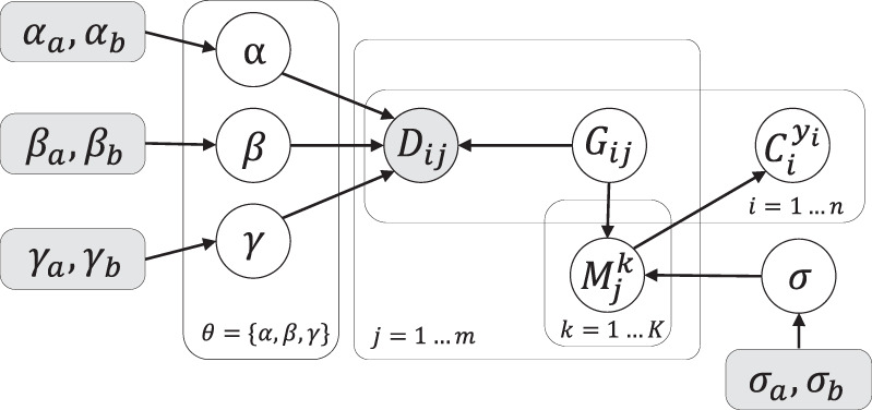
To achieve this goal, SCsnvcna uses a probabilistic model and Markov chain Monte Carlo (MCMC) to sample the placement of the SNVs on the edges of the CNA tree and the latent variables G, θ, and σ, in which G is the underlying genotype matrix; θ is a set of SNV cell error rates including FP rate α, FN rate β, and missing rate γ; and σ models the standard deviation of the cellular prevalence (CP) difference between SNV cells and CNA cells. Figure 1 gives an illustration of the model. In particular, given the input matrix D and the CNA tree, the MCMC searches for the true underlying G matrix, the placement of SNVs, the placement of SNV cells, and the placement of the latent variables θ and σ in an iterative fashion. In the Methods section, we describe in more detail the incorporation of single-cell errors (θ), the standard deviation of CP difference between CNA and SNV cells (σ), and the consideration of mutation loss owing to copy number loss.

Figure 1.

Illustration of SCsnvcna method. Inputs are observed data D (a cell-by-SNV matrix) and a CNA tree. Observed data may have FP SNVs (red 1s), FN SNVs (blue 0s), and missing entries (X). The underlying genotype matrix G along with the CP is initialized based on D. SCsnvcna places SNVs on the edges of the CNA tree (blue box) and SNV cells on the leaves of the CNA tree (orange box), followed by the update of the latent variables, which are G, the error rates θ, and the standard deviation of the CP difference between CNA cells and SNV cells (σ). The output of SCsnvcna is the placement of SNVs and cells on the CNA tree and the predicted values of G, θ, and σ.

Simulation results

We developed a simulator described in the Supplemental Methods, Section 1, to comprehensively test SCsnvcna under different conditions. We varied 15 variables in the simulation and broke them into five groups (Methods; Supplemental Methods, Section 2; Supplemental Table S1) for testing SCsnvcna and compared them with seven state-of-the-art methods: SCARLET (Satas et al. 2020), COMPASS (Sollier et al. 2023), SiFit (Zafar et al. 2017), SCG (Roth et al. 2016), RobustClone (Chen et al. 2020), SiCloneFit (Zafar et al. 2019), and BitSC² (Supplemental Methods, Section 3; Chen et al. 2022). Among these methods, SiFit and SiCloneFit only take SNVs as the input and do not infer the phylogenetic tree based on any CNA signal. RobustClone takes either SNV data or CNA data as the input, but not both. SCG only clusters SNV cells from SNV signal but does not infer a tree. We included these methods so that we can compare SCsnvcna with those methods taking only one source of data (SNV cells) as the input. Because SCsnvcna also takes CNA cells as the input in addition to SNV cells, SCsnvcna is expected to perform better than these methods. Similarly, SCARLET, COMPASS, and BitSC² are also designed to take both SNV and CNA signal as the input. Unlike SCsnvcna, which separates the steps of inferring a tree based on CNA signal and placing the SNVs on the CNA tree, these methods infer a tree considering SNV and CNA signals simultaneously. Although theoretically more advantageous, consideration of both signals at the same time requires an extremely large search space, which may hinder the ability to achieve the desired global minimum even after searching for a solution for a long time. To empirically check the performance of SCsnvcna compared with these seven methods, we applied them as well to the 15 simulated data sets whenever the data sets fit the methods. Notice that although Phertilizer (Weber et al. 2023) is also a method that combines SNV and CNA signals to infer a clonal tree, it was developed for high-throughput ultra-low-coverage data, which does not capture much of the needed SNV data. Therefore, we did not include Phertilizer in our comparisons.

Results from the simulated data with sequencing error (group 1), different scales (group 2), and biological challenges (group 3)

Three performance metrics have been measured to compare the eight methods, which are genotype error, pairwise SNV error, and pairwise SNV/CNA error (Methods). Figure 2 shows the performance of the methods on a varying FP rate, FN rate, and missing rate of SNVs, measuring the robustness of the methods in terms of sequencing error on SNV cells. Figure 3 shows the performance of the methods on a varying number of tree leaves, number of SNV cells, and number of SNVs, measuring the scalability of the methods. Figure 4 shows the performance of the methods on a varying percentage of CNAs detectable by SNV cells, varying mutation loss rate, and varying beta splitting variable, measuring the robustness of the methods in terms of challenges from the biological process of forming the tree. More description of these variables can be found in the simulation process in the Supplemental Methods, Section 1.

Figure 2.

Group 1: evaluation of methods given varying sequencing errors. Genotype error, pairwise SNV error, and pairwise SNV/CNA error are shown for SCsnvcna, SCARLET, COMPASS, SiFit, SCG, RobustClone, and SiCloneFit on varying FP rate (A), varying FN rate (B), and varying missing rate (C).

Figure 3.

Group 2: evaluation of scalability. Genotype error, pairwise SNV error, and pairwise SNV/CNA error are shown for SCsnvcna, SCARLET, COMPASS, SiFit, SCG, RobustClone, SiCloneFit, and BitSC² on varying number of tree leaves (A), varying number of SNV cells (B), and varying number of SNVs (C).

Figure 4.

Group 3: evaluation of methods given biological challenges. Genotype error, pairwise SNV error, and pairwise SNV/CNA error are shown for SCsnvcna, SCARLET, COMPASS, SiFit, SCG, RobustClone, and SiCloneFit on varying percentage of CNAs detectable by SNV cells (A), varying mutation loss rate (B), and varying beta splitting variable (C).

For the first group of data sets investigating the robustness of the methods in terms of sequencing error, we first varied FP rate in the SNV data. We found that SCARLET was very sensitive to FP rates (Fig. 2A). Its genotype error increased from 0.019 to 0.676 when the FP rate increased from 0.001 to 0.05. Similarly, we observed an increase of both pairwise SNV error (about 0.85) and pairwise SNV/CNA error (about 0.7) for SCARLET when the FP rate increased from 0.001 to 0.05. Like SCARLET, COMPASS was sensitive to FP rate (Fig. 2A). Its genotype error increased from less than 0.1 to more than 0.2 when the FP rate increased from 0.001 to 0.05. In contrast, SCsnvcna was robust to the FP rate. Its genotype error remained less than 0.033 for all FP rates, whereas both of its pairwise SNV error and pairwise SNV/CNA error remained below 0.1 for all FP rates. We then varied FN rate while fixing FP rate to its default value (Supplemental Table S1). In this experiment, we found that SCsnvcna was more sensitive to FN rate than was SCARLET (Fig. 2B). SCsnvcna's genotype error increased from 0.002 to 0.06 when the FN rate increased from 0.1 to 0.3. However, even at the FN rate of 0.3, SCsnvcna's genotype error was still greater than 0.1 lower than that of SCARLET under the same condition. Similarly, SCsnvcna's pairwise SNV error was greater than 0.2 lower than SCARLET's, and its pairwise SNV/CNA error was greater than 0.1 lower than that of SCARLET when FN rate was 0.3. In the third experiment in this group, we varied the missing rate of SNVs and found that SCsnvcna was robust to missing rate (Fig. 2C). Its pairwise SNV/CNA error increased slightly with the increasing missing rate, but even when the missing rate was as high as 0.3, its pairwise SNV/CNA error remained within 0.05, still about 0.2 lower than that of SCARLET.

For the second group of data sets investigating the scalability of the methods, we first varied the number of leaves on the tree. We found that BitSC² not only failed to place CNAs on the tree but also was not scalable to any tree that has 16 or more leaf nodes (Fig. 3). Similarly, SCARLET was not scalable to any tree that has 32 or more leaf nodes as the runs all terminated with errors but without results (Fig. 3A). In contrast, SCsnvcna can accommodate all numbers of leaves in this experiment. We then fixed the number of leaves to be the default value (Supplemental Table S1) and varied the number of SNV cells in the second experiment and the number of SNVs in the third experiment in this group. We observed that SiFit was extremely sensitive to the number of cells when the number of mutations was fixed (Fig. 3B). Its genotype error increased from less than 0.05 to more than 0.1, and pairwise SNV error increased from about 0.11 to about 0.829 when the number of SNV cells increased from 50 to 500. On the other hand, SiFit's performance greatly improved when the number of SNVs increased, whereas the number of SNV cell was fixed (Fig. 3C). Its pairwise SNV error decreased from about 0.413 to about 0.093 when the number of SNVs increased from 20 to 200. The combination of these two experiments showed that SiFit cannot render good performance when the SNV signal is lacking. In contrast, SCsnvcna was much more robust in both experiments; that is, its genotype error was within 0.05, and its pairwise SNV error was within 0.2 for all variables for these two experiments (Fig. 3B,C), showing the robustness and scalability of SCsnvcna in terms of varying SNV cell number and SNV number.

For the third group of data sets investigating the robustness of the methods in the face of different biological challenges, we first tested SCsnvcna's performance when changing the percentage of CNAs detectable by SNV cells (Methods; Supplemental Methods, Section 1). We found that SCsnvcna's pairwise SNV error and pairwise SNV/CNA error decreased with the increase of the percentage of CNAs detectable by SNV cells (Fig. 4A). This is expected because the more CNAs that are detectable by SNV cells, the more constraints SCsnvcna will find for the placement of SNV cells. However, even when there was no constraint of the CNAs, cases in which the percentage of the CNAs detectable by SNV cells was zero, SCsnvcna's genotype error was still within 0.1, much lower than that of SCARLET and COMPASS. Under the same circumstance, its pairwise SNV error was within 0.2, which was the lowest among all methods, and its pairwise SNV/CNA error was slightly better than that of SCARLET. Notice that SCARLET uses only one set of cells and thus requires that both CNAs and SNVs are detectable within the same set of cells simultaneously as explained also in the Supplemental Methods, Section 3.1. We then varied the mutation loss rate to test how robust SCsnvcna is in the face of different degrees of mutation losses in the data set (Supplemental Methods, Section 1). We found that SCsnvcna's pairwise SNV error and pairwise SNV/CNA error increased slightly with the increase of mutation loss rate (Fig. 4B). This is expected: As there are more mutation losses, the more challenging it is for SCsnvcna to place the SNVs correctly. We observed a similar trend on SCARLET on pairwise SNV/CNA error, although SCARLET's pairwise SNV/CNA error was much higher than that of SCsnvcna. The third experiment in this group was to test the performance of SCsnvcna in situations of contrasting subclone sizes on the leaf level, controlled by beta splitting variable (Supplemental Methods, Section 1). The larger the beta splitting variable, the more similar the subclone CPs are to each other (Fig. 4C). Similar CPs of subclones pose a challenge for SCsnvcna because the smaller the contrast of the CPs, the less identifiable the subclones. As expected, we observed SCsnvcna had an increasing pairwise SNV/CNA error in the increasing of the beta splitting variable. Although SCsnvcna relies on the CPs in placing SNV cells, SCsnvcna's genotype error remained very low (∼0.08) when the beta splitting variable was as high as 0.5. Under the same circumstances, its pairwise SNV error and pairwise SNV/CNA error were both within 0.1 compared with SCARLET's, which were above 0.4 and 0.2, respectively.

In all of the above-mentioned three groups of data sets, SCG achieved a very low genotype error (less than 0.05) in almost all cases. However, SCG cannot estimate the pairwise SNV relationship. Neither does it infer a tree structure. Thus, the application of SCG is most useful for clustering SNV cells and achieving the consensus genotype for each cluster. RobustClone's pairwise SNV error was the highest among all methods for all experiments, and they were greater than 0.7 for all cases except when tree leaf number was eight compared with SCsnvcna, whose pairwise SNV error was less than 0.15 for a majority of cases. We further looked into RobustClone's intermediate result and found that RobustClone did not place a large number of SNVs on the tree, whereas these SNVs had very small impact on the genotype error. This explains why RobustClone can achieve relatively low genotype error (less than 0.1 for most of the experiments) while having a high pairwise SNV error. In addition, because RobustClone takes either SNVs or CNAs as the input but not both, it does not infer CNAs on the tree. Therefore, we did not report the pairwise SNV/CNA error for RobustClone.

SiCloneFit achieved a comparably low genotype error for almost all variables except when the SNV number was at the low value of 20 (genotype error was near 0.05). However, its pairwise SNV error was very high (0.2–0.5). After further investigation, we found that 30%–50% of the pairwise SNV error was owing to the fact that SiCloneFit mistakenly predicted the mutations to be parallel mutations, and some mutations were not placed on the tree at all, the latter of which tended to have small VAFs (less than 0.1). Thus, we conclude that SiCloneFit reached a low genotype error mainly by adding parallel mutations or not placing the mutations with low VAFs at all.

In summary, from the first three groups of simulated data sets, we found that SCsnvcna stood out among the comparison methods in that it achieved (1) consistently low genotype error, (2) consistently lowest pairwise SNV error, (3) relatively accurate inference of pairwise SNV/CNA relationship, and (4) robust scalability when tested with a wide range of values of tree leaves, SNVs, and SNV cells.

Results from the simulated data with large CP differences (group 4) and imperfect CNA tree (group 5)

In addition to the parameters examined in the previous three groups of data sets, we examined SCsnvcna's performance in comparison with other methods when the CP difference between SNV cells and CNA cells is larger than that is modeled (group 4), and when the CNA tree structure is imperfect for SNV placement (group 5). Thus, this section focuses on the imperfect cases in the face of large difference between SNV cells and CNA cells in terms of their CPs and placement on a tree. First, for group 4, we conducted experiments that mimicked the sampling bias between SNV cells and CNA cells, which included three data sets. The first data set assumed that the CP difference was according to a Gaussian distribution whose standard deviation was a variable that we varied. The second data set assumed that the CP difference was not according to a Gaussian distribution but a Gaussian distribution plus a beta distribution. Because none of the other methods were affected by CP difference between SNV cells and CNA cells, we did not compare with other methods in this group of experiments. Instead, we showed our results to investigate how much the error rates may vary with the varying variables. In the previous two data sets in group 4, we treated the CNA cells’ CPs the same as true CPs. In reality, the CNA cells’ CPs may differ from the true CPs owing to the sampling bias. The third data set assumed that both the CNA cells’ CPs and the SNV cells’ CPs differed from the true CPs, and were draw from a multinomial distribution.

In the first data set, we varied the standard deviation of the Gaussian distribution of the CP difference between SNV cells and CNA cells from 0.01 to 0.1. As seen in Supplemental Figure S1A, SCsnvcna was robust to both small and big standard deviations, and there was not an obvious trend of SCsnvcna's performance with respect to the standard deviations.

Given that the difference of the CPs between SNV cells and CNA cells can be much bigger than that a Gaussian distribution models, we designed a simulation experiment in the second data set of group 4 that imputed a Gaussian plus a beta distribution of the CP difference between SNV cells and CNA cells (Supplemental Methods, Section 2.2). Thus, a node's CP difference between SNV cells and CNA cells differed not only by a Gaussian distribution but also by a ratio sampled from a beta distribution. As shown in Supplemental Figure S1B, SCsnvcna's error rates did not change significantly when the mean of the beta distribution increased from zero to 0.8, showing the robustness of SCsnvcna in the face of large non-Gaussian CP difference between SNV cells and CNA cells. Moreover, SCsnvcna's genotype error rate remained within 0.1 and pairwise SNV error fluctuated around 0.2, showing that SCsnvcna maintained its high accuracy in the face of large CP differences that SCsnvcna did not model.

Previous experiments did not impose any CP difference between the CNA cells and the underlying true CP (Supplemental Methods, Section 1). In reality, it is possible that the CNA cells’ CPs differ from the true CP. Moreover, the difference between the SNV/CNA cells’ CPs and the true CPs may not be corresponding to a Gaussian distribution. In the third experiment, we tested SCsnvcna's performance when both the SNV cells’ CPs and the CNA cells’ CPs differ from the true CP by a non-Gaussian distribution (Supplemental Methods, Section 2.3), and compared our result with SCARLET and COMPASS as these two methods can take both CNA and SNV signals simultaneously. We found that with such a setting in which both CNA cells’ CPs and SNV cells’ CPs differ from the true CPs, our genotype error stays lower than 0.06 compared with SCARLET's (greater than 0.2) and COMPASS's (greater than 0.12) (Supplemental Fig. S1C). Our pairwise SNV error increases to a little lower than 0.2, but it is still much lower than that of SCARLET (0.44) and COMPASS (0.38). As expected, our pairwise SNV/CNA error increases the most, to 0.225. However, it is still lower than that of SCARLET, which is more than 0.25.

In addition to large CP differences between SNV cells and CNA cells, in the real case scenario, it is also possible that the CNA tree's structure differs greatly from the underlying phylogenetic tree, owing to either missing CNA subclones because of the sampling bias or the lack of the CNAs that can distinguish two subclones of SNV cells. To examine SCsnvcna's performance in such situations, we simulated three data sets that are grouped into group 5. These three data sets examined the cases in which some branches on the true phylogenetic tree did not have CNAs to distinguish two subclones, some of the leaf nodes on the CNA tree were missing owing to sampling bias, and the CNA tree was a bulk CNA tree (Supplemental Fig. S2).

The first experiment in group 5 simulates the case when the CNAs that can distinguish two SNV cells are lacking; in other words, there are some subclones that can be distinguished by SNVs but not CNAs (Supplemental Methods, Section 2.4). Such a situation is possible when two sets of cancer cells share a set of CNAs but not necessarily so for the SNVs. Therefore, these cancer cells are distinguishable by SNVs but not CNAs. Because SCsnvcna does not aim at correcting the CNA tree structure, we designed the following experiment to test the robustness of SCsnvcna when there are no corresponding edges/nodes in the CNA tree for SNVs.

The purpose is to examine SCsnvcna's performance when the CNA tree does not have all edges where the SNVs could have been placed. We ran SCsnvcna on the CNA tree along with other methods and showed the results in Supplemental Figure S2A. We did not run SiFit, SCG, RobustClone, and SiCloneFit on this set of simulated data because their algorithms do not use both CNA and SNV signal. We did not run BitSC² as it was not scalable to a tree with 16 leaf nodes. Instead, we compared with SCARLET and COMPASS, both of which took into account the CNA signal. We found that although SCsnvcna's genotype error and pairwise SNV error increased with the increase of percentage of internal nodes whose child nodes were deleted, its error rate remained among the lowest regardless of the percentage values. Notably, SCsnvcna was the only method that had a genotype error less than 0.1 when 50% of the internal nodes’ child nodes were deleted. Its pairwise SNV error was similarly favorable at less than 0.3 when 50% of the internal nodes’ child nodes were deleted. In this experiment, we found that COMPASS was robust to the changing CNA tree structure. This was expected as COMPASS did not take a CNA tree structure as the input. Instead, it estimated the CNAs given the read counts on each targeted region. However, SCsnvcna's genotype error and pairwise SNV error were smaller than COMPASS's for all cases tested in this experiment, even at the highest percentage of internal nodes whose child nodes were removed. In all, although SCsnvcna's performance was sensitive to a CNA tree structure that does not have all edges where the SNVs should have been placed, it outperformed SCARLET and COMPASS in all values of percentage of internal nodes whose child nodes were removed. This shows that SCsnvcna is eligible to be applied to the situation when the CNA tree does not necessarily have all edges to distinguish two subclones.

The first experiment in this group focused on the lack of the CNAs to distinguish two subclones. For the second experiment in this group, we focused on the case when the sampling bias during the sequencing of cells led to missing CNA subclones in the CNA tree. Sampling bias of the CNA cells may occur when the cells are sampled and distributed for SNV detection and CNA detection, leading to that one or more of the subclones at not being represented by any CNA cells. Subsequently, the inferred CNA tree lacks the leaf nodes to represent the missing subclones. To test SCsnvcna's performance in the presence of missing leaf nodes in the CNA tree, we removed a certain percentage of leaves on the CNA tree according to the CPs of the leaf nodes (Supplemental Methods, Section 2.5). Such a percentage was a variable that we varied in this experiment. Supplemental Figure S2B showed the genotype error, pairwise SNV error, and pairwise SNV/CNA error of applying SCsnvcna to the CNA tree that lacked leaf nodes to different percentages. In this experiment, we did not compare with SCARLET and COMPASS because they do not distinguish SNV cells and CNA cells, and thus, lacking CNA cells means lacking both SNV cells and CNA cells. As shown in the figure, SCsnvcna's genotype error remained below 0.05 for all three percentages (10%, 25%, and 50%) of missing leaf nodes being tested, and their difference from each other was very small (less than 0.01). This showed that SCsnvcna is robust to missing leaf nodes on the CNA tree. SCsnvcna's pairwise SNV error and pairwise SNV/CNA error did not show a clear trend, whereas the pairwise SNV error was around 0.2 and pairwise SNV/CNA error was around 0.25. In summary, SCsnvcna was robust to a CNA tree that lacked some leaf nodes owing to the sampling bias.

In the next experiment, we evaluated how SCsnvcna may perform when the CNA tree was from multisample bulk sequencing, called “bulk tree” in the following text (Supplemental Methods, Section 2.6). This experiment is interesting because when the single-cell sequencing for CNA detection is lacking, the CNA tree inferred from single-cell sequencing (called “single-cell CNA tree” in the following text) may be replaced with the bulk tree should the latter exists. The major difference between a bulk tree and a single-cell CNA tree is that a bulk tree does not render accurate CPs and that a bulk tree may not render as many leaf nodes as a single-cell CNA tree, both of which are owing to the lack of samples compared with the number of single cells. It is expected that when the leaf node number is small, some subclones are not represented by the bulk samples, and the SNVs unique to those missing subclones cannot be placed correctly on the corresponding bulk tree. Supplemental Figure S2C showed results when the number of bulk samples is four and eight. The results of SCsnvcna that took the original single-cell CNA tree that had 16 leaf nodes as the input were also shown as the reference. As expected, the smaller the number of bulk samples, the higher the genotype error and pairwise SNV error (Supplemental Fig. S2C). However, SCsnvcna's genotype error was within 0.1 for all number of bulk samples in this experiment. The pairwise SNV error dropped from more than 0.5 to less than 0.2 when the number of bulk samples increased from four to eight, showing the importance of having multiple bulk samples representing different subclones for an accurate SNV placement when the input tree was a bulk tree. Because a big portion of the CNAs were missing in the bulk tree, we did not evaluate the pairwise SNV/CNA error for this experiment.

Results from the simulated data generated by a different simulator

To further show SCsnvcna's robustness to different data sets, we used a different simulator from ours as reported by Sollier et al. (2023) to generate additional simulated data sets for orthogonal validation (Supplemental Methods, Section 5). In total, we simulated three data sets using the simulator reported by Sollier et al. (2023) to test the robustness of our method, varying the number of cells, number of mutations, and number of nodes on the tree (Supplemental Methods, Section 5). We then ran SCsnvcna on the three sets of the simulated data in two ways, with and without constraining the SNV cell placement, and compared with COMPASS and BiTSC². Notice that both COMPASS and BiTSC² assumed that the SNVs and CNAs were detected from the same set of cells and, thus, fixed the SNV cell placement. Therefore, the run of SCsnvcna with constraining the SNV cell placement had a fairer comparison with COMPASS and BiTSC² than the run without constraining the SNV cell placement. In this experiment, we did not compare with SCARLET because the simulator does not provide the list of potential loss of mutations owing to loss of copies, which was required by SCARLET.

As shown in Supplemental Figure S3A, SCsnvcna's performance was the best of all methods tested when the SNV cells were constrained. Even when no SNV cell was constrained, SCsnvcna's performance was still comparable to COMPASS’. BiTSC²'s performance was much worse than the other methods when the SNV cell number was greater than 100.

We observed from Supplemental Figure S3B that COMPASS’ genotype and pairwise SNV error rates increased quickly when the number of mutations increased to 200, whereas SCsnvcna was robust to varying numbers of mutations. We also observed that BiTSC² achieved much lower error rates when the number of mutations increased to 100. The combination of varying number of cells and varying number of mutations showed that BiTSC² performs worse when the number of SNV cells increases or when the number of mutations decreases, whereas COMPASS had the opposite trend. In the simulated data sets proposed in this paper, we also observed the COMPASS’ performance declined when the number of mutations increased.

Lastly, Supplemental Figure S3C showed the result when we varied the number of subclones between eight and 16. We found that COMPASS’ genotype and pairwise SNV error rates increased when the number of subclones increased to 16. Just as the previous simulated data sets showed, BiTSC² failed to produce any result when the number of subclones was 16. However, SCsnvcna consistently performed well for the cases of both eight and 16 subclones. Consistent with the previous observations, SCsnvcna performed the best of all methods tested when the SNV cells were constrained.

Because the data created by this simulator has both SNVs and CNAs on the same cell in the ground truth, we further evaluated whether SCsnvcna assigns the SNVs and CNAs to each cell correctly. To be specific, we calculated the recall, which evaluated the percentage of SNVs that was correctly assigned to a cell among all SNVs that a cell truly contained, and the precision, which evaluated the percentage of the true SNVs a cell contained among all SNVs that were assigned to the cell. We also evaluated the recall and precision for CNAs similarly to the SNVs. We found that >72% cells had greater than 0.8 recall and precision for both SNVs and CNAs, showing that SCsnvcna by large correctly placed the SNV cells and SNVs.

In summary, given the simulator published by Sollier et al. (2023), we observed similar trends of SCsnvcna, COMPASS, and BiTSC² as to what we observed in the data sets simulated by the simulator reported along with this study. With the three sets of data simulated, we found that SCsnvcna consistently produced results with low genotype and pairwise SNV errors and was the most robust of all methods tested.

Mutation loss detection

In addition to genotype error, pairwise SNV error, and pairwise SNV/can error, we also measured the sensitivity and specificity of SNV loss detection for SCsnvcna and SCARLET. We did not measure the SNV loss detection accuracy for the other methods because they did not detect SNV loss owing to copy number loss. The results have been shown in Supplemental Figure S4. Although SCsnvcna's sensitivity of SNV loss detection was not as high as SCARLET's, its specificity was higher than that of SCARLET. In fact, its specificity stayed between 0.9 and 1.0 for almost all 11 experiments. Thus, we concluded that SCsnvcna is more conservative in predicting SNV losses than is SCARLET. Achieving a more sensitive detection of SNV loss is a future extension work of SCsnvcna.

Real data experiment: CRC patient tumor data

The two scDNA-seq data sets on metastatic colorectal cancer, the CRC1 and CRC2 patient tumor data sets (Leung et al. 2017), serve perfectly the purpose of this study because they both contain CNA cells and SNV cells sampled from the same patient, respectively. To be more specific, for both CRC1 and CRC2 patient tumor data sets, CNA cells and SNV cells were sequenced from different single-cell sequencing technologies. The CNA cells were sequenced by the single-nucleus sequencing (SNS) (Navin et al. 2011), whereas the SNV cells were sequenced by highly multiplexed scDNA-seq (Leung et al. 2016), targeting 1000 cancer gene panel that resulted in 137× of mean coverage depth and 0.92 of average coverage breadth (Leung et al. 2017).

In addition, the CRC2 data set is composed of a primary tumor sample and two metastatic samples (called M1 and M2), and there have been controversial conclusions regarding whether there have been “bridge mutations” in between the two metastases, that is, whether the primary tumor continued to gain more mutations after the first metastasis occurred and reseeded, which led to the second metastasis. We therefore are interested in applying SCsnvcna to CRC2 to investigate the data by considering both CNAs and SNVs on the same phylogenetic tree.

Applying SCsnvcna to CRC patient tumor data sets

In the following, we describe how we applied SCsnvcna to the CRC2 patient tumor data set, as well as the CRC1 patient tumor data set. Because the CRC2 sample has sequencing data from both the primary colon tumor and two metastasis tumors, we used the aneuploid SNV and CNA cells from all three sites.

We used a total of 42 CNA cells in our CNA analysis from the primary colorectal/colon tumor site and liver metastasis sites in our CNA analysis. Sixty-seven SNV cells and 30 SNV sites were included as our input to SCsnvcna. Notice that we used the CNA cells from all three tumors (primary, M1, and M2) of the same patient sample for inferring the CNA tree without fixing their genealogical order. This allows for primary cells to be in a parallel branch of the metastasis cells or even occur later than the metastasis cells. Because the diagnosis of the primary tumor and the two metastatic tumors in CRC2 occurred at the same time (Leung et al. 2017), the primary tumor cells may have evolved after the metastasis happened, as also recognized by Leung et al. (2017). Therefore, instead of assuming that all primary cells stay closer to the root than M1 and M2, we used MEDICC2 (Kaufmann et al. 2022) to infer the CNA tree based on all CNA cells in order to best explain the lineage of the primary cells and the two sets of metastatic cells in CRC2.

The CRC1 data set has the tumor cells from both the primary tumor (colon) and metastatic site (liver) (Leung et al. 2017). In total we used 66 SNV cells and 31 CNA cells, and a total of 15 SNVs were identified from the SNV cells, which served as the input to SCsnvcna. Like CRC2, the CNA cells from both the primary tumor and metastasis were used for inferring the CNA tree by MEDICC2, and no prior knowledge of their genealogical order was given to MEDICC2.

Results of CRC2 patient tumor data set

A simplified phylogenetic tree as the output of SCsnvcna on CRC2 is shown in Figure 5. A detailed phylogenetic tree with the labels of the single cells is shown in Supplemental Figure S5.

Figure 5.

A simplified phylogenetic tree for CRC2 inferred by SCsnvcna. Circles represent the tumor clones. Metastatic cells belonging to M1 and M2 are highlighted in magenta and orange, respectively, whereas all other nodes represent cells in the primary tumor. The genes of CNAs and SNVs are annotated on the edges of the tree. SNVs are highlighted with the blue background. CNAs are in the white background. Copy number gains and losses are grouped in each line and are denoted by a leading “+” and “−” sign, respectively.

Consistent with the published findings (Leung et al. 2017), SCsnvcna also inferred a polyclonal seeding on the liver and bridge mutations on the trunk after the first metastasis but before the second one. More specifically, SCsnvcna inferred that SNVs in NRAS, CDK4, APC.1, TP53, MYH11, and LINGO2.1 occurred before the gain of copies on oncogenes BCL9, ABL2, ETV5, PIK3CA, and BCL6. Subsequently, SCsnvcna placed SNVs in STRN and MN1 on the trunk. SCsnvcna then inferred that there was a seeding to M1 after the gain of mutation in LINGO2.2. On the trunk after this seeding, SCsnvcna inferred the gain of mutations in CHN1, FHIT, and APC.2, the bridge mutations that were also inferred by Leung et al. (2017) before the second seeding that led to M2.

Regarding the placement of the SNVs on M1, SCsnvcna and the results from Leung et al. (2017) were consistent in placing the SNVs in LINGO2.2, LINGO2.3, F8, SPEN, LAMB4, PIK3CG, PTPRD, LINGO2.4, and IL7R. In addition, like Leung et al. (2017), SCsnvcna also placed the SNV in LINGO2.2 on top of the M1 cells, consistent with the interpretation that LINGO2.2 was an initiating mutation contributing to the first metastasis in the liver.

Similarly, the analysis of M2 showed that the SNVs in NR4A3, FUS, PRKCB, TSHZ3, and HELZ were placed on M2 by both SCsnvcna and Leung et al. (2017). Unlike Leung et al. (2017), SCsnvcna placed ATP7B at the start of M2 instead of on the main branch as a bridge mutation. Although the work of Leung et al. (2017) showed strong read count support that the SNV in ATP7B occurred in M2 but not in M1, it failed to show that ATP7B occurred in the primary tumor cells as well. In fact, as shown by Leung et al. (2017), there were only four out of 18 primary tumor cells that had strong support of having ATP7B. Thus, our placing ATP7B at the start of M2 has more biological support compared with considering it as a bridge mutation, illustrating the power of SCsnvcna to refine SNV placement and bridge mutation determination in complex multitumor samples.

After the occurrence of M2, both SCsnvcna and Leung et al. (2017) inferred that the primary tumor cells continued to gain more SNVs in LINGO2 and LRP1B (listed as UAP1B in Leung et al. 2017), confirming that these SNVs were the last few gained in primary tumor cells before the synchronized diagnosis and tumor resection occurred.

We note that the SNVs in CHN1, FHIT, and APC2, although classified as bridge mutations by Leung et al. (2017) and confirmed by SCsnvcna, were not indicated as bridge mutations by SCARLET (Satas et al. 2020). Instead, SCARLET placed the SNVs in CHN1, FHIT, and APC on the trunk before M1 occurred, and inferred that they were not detected in M1 cells owing to copy number losses on M1 branches. However, such an explanation is not consistent with the copy number states, which are the same for M1 and M2 for each of the bridge mutations mentioned above (Leung et al. 2017).

We then investigated SCsnvcna's placement of SNV cells by comparing their clustering result with the anatomical origin from the patient. We found that SCsnvcna grouped the SNV cells into three main clusters: primary, M1, and M2, consistent with the resection sites in the patients. Specifically, 13 out of 15 cells that were clustered by SCsnvcna have been categorized as M1 by Leung et al. (2017). SCsnvcna clustered 12 out of 13 SNV cells that were classified as M2 by Leung et al. (2017).

Results of CRC1 patient tumor data set

A simplified phylogenetic tree as the output of SCsnvcna on CRC1 is shown in Figure 6. A detailed phylogenetic tree with the labels of the single cells is shown in Supplemental Figure S6.

Figure 6.

A simplified phylogenetic tree for CRC1 inferred by SCsnvcna. Circles represent the tumor clones. Metastatic cells are highlighted in orange, whereas all other nodes represent cells in the primary tumor. The genes of CNAs and SNVs are annotated on the edges of the tree. SNVs are highlighted with the blue background. CNAs are in the white background. Copy number gains and losses are grouped in each line and are denoted by a leading “+” and “−” sign, respectively.

Consistent with the work of Leung et al. (2017), SCsnvcna inferred two subclones, the primary tumor and metastasis. Specifically, consistent with work of Leung et al. (2017), SCsnvcna placed SNVs at APC, KRAS, TP53, FAT3, MYH9, TDRP, CCNE1, ROBO2, and TCF7L2 on the trunk. SCsnvcna then inferred that there was a seeding to metastasis after the gain of mutation in POU2AF1. This is consistent with the timing of the metastasis inferred by Leung et al. (2017). On the trunk after this seeding, SCsnvcna inferred the gain of a mutation in TPM4, consistent with work of Leung et al. (2017).

On the metastatic tumor, SCsnvcna placed five SNVs: SNVs at RBFOX1, ZNF521, EYS, TRRAP, and GATA1. These five SNVs were the same as those placed on metastasis by Leung et al. (2017). In terms of SNV cell placement, SCsnvcna placed all SNV cells to their corresponding CNA subclones; that is, primary SNV cells were placed on the primary subclone, whereas metastatic SNV cells were placed on the metastatic subclone.

Discussion

We developed SCsnvcna, an open-source computational tool that places SNVs and SNV cells on a CNA tree for scDNA-seq data. The algorithm is based on the following: that the SNV cells and CNA cells from the same subclone shall have close CPs and that the SNV cells evolve along a tree, and thus, the SNVs shall be constrained on a tree. SCsnvcna takes into account the scDNA-seq-specific errors such as FP and FN rates, the missing errors, and the potential loss of SNVs owing to copy number losses. Moreover, SCsnvcna can use the limited CNA signal from the SNV cells to constrain the SNV cell placement on a CNA tree. Finally, SCsnvcna was designed to model and thus tolerate the sampling bias between CNA and SNV cells.

Fifteen simulated data sets have been used to examine the performance of SCsnvcna in comparison with seven state-of-the-art methods: SCARLET, COMPASS, SiFit, SCG, RobustClone, SiCloneFit, and BitSC². We found that SCsnvcna's performance was robust with regard to sequencing error rates, CP differences between SNV cells and CNA cells, and various imperfect CNA tree structures. Moreover, SCsnvcna is scalable to a wide range of values of leaf nodes, SNVs, and SNV cells. In most of the cases, including those that SCsnvcna is sensitive to such as imperfect input tree structure and varying CP differences between SNV cells and CNA cells, SCsnvcna's genotype error rate, pairwise SNV error rate, and pairwise SNV/CNA error rate were among the lowest of all methods. In addition, we tested SCsnvcna on an orthogonal simulated data set and found that SCsnvcna consistently generated results with low genotype and pairwise SNV errors. In all, SCsnvcna is the only method of all eight that has a good balance of high accuracy, robustness, and scalability.

We applied SCsnvcna to the CRC2 and CRC1 patient tumor data sets. On the CRC2 patient tumor data set, we found that SCsnvcna's placement of SNVs was consistent with that of Leung et al. (2017). SCsnvcna also correctly placed most of the cells, which clustered into primary and two metastasis groups that were consistent with their anatomical sites. SCsnvcna inferred three “bridge” SNVs on the trunk between the two metastases, which was consistent with the conclusion from the original study on CRC2 by Leung et al. (2017), thus confirming that there was a bridging and reseeding process after the first metastasis was formed. However, SCsnvcna did not infer the SNV at ATP7B as a bridge mutation like Leung et al. (2017). Instead, SCsnvcna inferred it to be placed at the start of M2. Such a placement has a stronger support from the sequencing data than placing the SNV at ATP7B as a bridge mutation. In the application of SCsnvcna to the CRC1 patient tumor data set, SCsnvcna correctly inferred the placement of the SNVs on both the primary and the metastatic CNA cell subtrees. SCsnvcna also placed the SNV cells at the positions consistent with their original resection sites.

We acknowledge that the existing state-of-the-art single-cell CNA detection tool does not always infer the ploidy and absolute copy number profile correctly. Although we manually corrected the ploidies for CRC2 data set based on the conclusion from Leung et al. (2017), we also provided a solution on how to detect wrongly inferred ploidies and how to correct them, seen in the Supplemental Methods, Section 6. We expect CNA detection tools will continue to be developed to strengthen the accuracy of ploidy inferences in the future.

We also noticed that in CRC2 data analysis, a few genes, such as CDX2, CDK8, and ABL2, have been predicted to be gained or lost more than once by MEDICC2. This is because MEDICC2 allows homoplasy and does not hold the infinite site assumption, making MEDICC2 more realistic in inferring a CNA tree (Kaufmann et al. 2022). As also stated by Mallory et al. (2020b), violations of infinite site assumption on CNAs are expected to occur much more frequently than SNVs. Further, such genomic instability is especially common in metastasis (Bakhoum et al. 2018). However, it is challenging to validate the genomic instability experimentally. To the best of our knowledge, MEDICC2 is the most advanced CNA tree inference tool so far that does not assume independent bins and thus allow overlapping CNAs, does not hold the infinite site assumption, does not limit the sequenced CNA profiles to have occurred in the internal nodes of the tree, and is also computationally efficient. That being said, SCsnvcna's implementation allows for the input of CNA trees from other methods and is not just limited to the one from MEDICC2. When more advanced CNA tree inference methods are developed in the future, SCsnvcna's performance may be further improved along with the increased accuracy of the input CNA trees.

One future work of improving SCsnvcna is to enhance its sensitivity to mutation loss detection. Specifically, for those mutation losses caused by copy number losses, comparing the read depth on the locus where the mutation losses occur with its flanking regions will help to identify and thus resolve the molecular and evolutionary nature of mutation losses.

Another interesting route for future development is to place CNAs on an SNV-based tree. We did not pursue this route because the CNA tree provides us with the information of copy number losses, which can guide the placement of SNVs in cases of mutation losses.

A third route is to jointly infer the phylogenetic tree, the placement of SNVs and CNAs, and the placement of SNV cells and CNA cells simultaneously. This route is even more necessary when a subtree on a phylogenetic tree lacks any CNA. In such a case, the CNA tree structure will not include such a subtree, leading to inaccurate placement of SNVs by SCsnvcna. Jointly inferring the phylogenetic tree is therefore needed because the resulting tree structure is formed by not only CNAs but also both CNAs and SNVs. Nevertheless, jointly inferring the phylogenetic tree will involve a much bigger solution dimension and thus will be computationally challenging. Developing computationally efficient solutions or using parallel computing will be considered to resolve such challenge.

Because it is possible that the data given is not only from scDNA-seq but also from the bulk sequencing, a fourth route is to infer a phylogenetic tree given the bulk sequencing data in addition to the scDNA-seq data, which are all from the same sample. Specifically, the variant allele fraction (VAF) of the SNVs inferred from the bulk sequencing data can serve as a constraint in placing the SNVs on the CNA tree in the sense that the VAF of a SNV shall be consistent with the CP of the same SNV from the scDNA-seq data. A more complex statistical model can be developed that involves such a comparison of the VAFs from the bulk sequencing and CPs from scDNA-seq.

Finally, we noticed that there is a trend of fully using the high-throughput ultra-low-coverage sequencing data alone to infer a clonal tree (Weber et al. 2023). Extending SCsnvcna to be applicable to such data without having high-coverage data is envisioned for future iterations of our methodology development.

In conclusion, SCsnvcna offers a powerful new computational phylogenetics tool that solves the challenge of integrating previously disparate single-cell data sets by placing SNVs on a CNA tree. SCsnvcna can validate and reveal interesting order and interplay between SNVs and CNAs in tumor progression and thus boost the understanding of how tumor gains new mutations and grows. With the decrease of the sequencing cost, SCsnvcna has shown value with potential for wide application to multiple scDNA-seq data sets, helping to advance our comprehension of the complex biology of tumor growth and intra-tumor heterogeneity.

Methods

Model of single-cell errors

The observed genotype matrix of SNVs D is different from the true underlying genotype matrix G, a n*m binary genotype matrix, owing to the sequencing errors. We model the errors in D as θ, where θ = {α, β, γ}, in which α, β, and γ represent FP, FN, and missing error rates. The probability of D given G and θ is described in Equation 1:

$$P(D_{i,j}|\theta ,G_{i,j})=\{\begin{array}{ll}\gamma ,& \mathrm{if}{D}_{i,j}=X,G_{i,j}=0\\ \gamma ,& \mathrm{if}{D}_{i,j}=X,G_{i,j}=1\\ 1-\alpha -\gamma ,& \mathrm{if}{D}_{i,j}=0,G_{i,j}=0\\ \beta ,& \mathrm{if}{D}_{i,j}=0,G_{i,j}=1\\ \alpha ,& \mathrm{if}{D}_{i,j}=1,G_{i,j}=0\\ 1-\beta -\gamma ,& \mathrm{if}{D}_{i,j}=1,G_{i,j}=1\end{array}$$ (1)

Using CP to place SNVs on a CNA tree

The CP of a SNV j, ${\overline{V}}_j$, can be calculated by Equation 2 given its true underlying genotype G_i,j for all cells:

$${\overline{V}}_j={\displaystyle \frac{\sum _{i=0}^n{G}_{i,j}}{n}}$$ (2)

Given the CP for a SNV j, SCsnvcna searches the most fitting branch on tree T to place SNV j. Specifically, suppose the percentage of CNA cells in T under an edge E_k is ${\hat{V}}_k$. We place SNV j on the edge E_k whose ${\hat{V}}_k$ is closest to ${\overline{V}}_j$. This is based on the assumption that SNV and CNA cells are from the same patient sample and, thus, the same underlying phylogenetic tree. To consider potential sampling bias, we model the distance between the two CPs, $d_{{\overline{V}}_j,{\hat{V}}_k}$, by a Gaussian distribution, which has zero mean and σ as the standard deviation. σ represents the sampling bias, which is a latent variable to be inferred by our MCMC sampling algorithm or given by the user.

Using the CNAs on SNV cells to limit the placement of SNV cells

Although the SNV cells are mainly for the detection of SNVs, it is still possible to detect some CNAs at a lower resolution. Should these CNAs overlap with those CNAs detected from CNA cells, SCsnvcna will constrain the SNV cells that contain these CNAs to the leaves whose CNA cells contain the same CNAs. Because the path from the root to the node where the SNV cell is placed spells out the SNVs that the cell carries, the placement of SNV cells constrains the placement of SNVs. Thus, the CNA signal on SNV cells, although limited, constrains not only the placement of SNV cells but also the placement of SNVs on the edges of the CNA tree.

Deciding which leaves on the CNA tree that the SNV cells are constrained to is a preprocessing step of SCsnvcna. We implemented two strategies to provide a list of leaf nodes, and users can choose either way should they provide the copy number profiles of both CNA cells and SNV cells. The first strategy is applicable when there are very limited number of CNAs detectable on the SNV cells. Specifically, for a SNV cell i, if one of its CNAs overlaps with a CNA u detected from CNA cells by at least p%, we limit the placement of the SNV cell i on only the leaves of the subtree whose root is the node below the edge where u occurs. If more than one CNA on the SNV cell i overlaps with those detected from CNA cells, the placement of cell i will be the intersection of the nodes constrained by each of the overlapping CNAs. Unlike the first strategy, to constrain a SNV cell to a CNA leaf node, the second strategy requires this SNV cell to contain >x% of the CNAs specific to this CNA leaf node. To infer the list of the CNAs specific to a CNA leaf node, an existing clustering method, such as HDBSCAN (McInnes et al. 2017), can be applied to cluster the CNA cells into different groups. Then, the list of unique CNAs for a group, A, can be identified by identifying the CNAs appearing in >y% of the cells in group A but appearing in <z% of the cells in all other groups. If a cell can be constrained to multiple leaf nodes, its placement will be within the range of the union of these leaf nodes. Section 7 in the Supplemental Methods describes how to tune x to achieve the most effective constraints of the SNV cells.

Loss of SNVs owing to copy number loss

It is possible that a SNV is lost owing to the copy number loss. Thus, all the SNV cells that obtained the SNV followed by a copy number loss may not show signal of this SNV on the D matrix any more. SCsnvcna is capable of detecting such SNV loss owing to copy number loss. Should SCsnvcna determine a certain SNV is lost owing to copy number loss, there is no penalty in the CP distance between the CNA cells and SNV cells; that is, the nodes under the edge of the copy number loss are not counted in calculating the CPs of CNA cells or SNV cells.

In the case of multiple equally good solutions while considering the loss of SNVs owing to copy number loss, we randomly select one of the best trees.

Probabilistic graphic model of SCsnvcna

Figure 7 shows the probabilistic graphic model of SCsnvcna.

Figure 7.

Probabilistic graphic model of SCsnvcna. Shaded nodes are given parameters or input data. Unshaded nodes are the latent variables to be inferred.

The distributional assumptions for all variables are as follows:

$$\begin{array}{rl}& \alpha |{\alpha }_a,{\alpha }_b\sim Beta({\alpha }_a,{\alpha }_b)\\ & \beta |{\beta }_a,{\beta }_b\sim Beta({\beta }_a,{\beta }_b)\\ & \gamma |{\gamma }_a,{\gamma }_b\sim Beta({\gamma }_a,{\gamma }_b)\\ & \sigma |{\sigma }_a,{\sigma }_b\sim Beta({\sigma }_a,{\sigma }_b),\\ & D_{ij}\sim E\left(D_{ij}\right|G_{ij},\alpha ,\beta ,\gamma )\\ & M_j^k\sim \prod _{i=1}^{n}P(M_j^k|G_{ij},\sigma )\\ & C_i^{y_i}\sim \prod _{j=1}^{m}P(D_{i,j}|y_i,M_j^k)\end{array}$$

where E denotes the error model in the data defined by Equation 1. α_a, α_b, β_a, β_b, γ_a, γ_b, σ_a, and σ_b are latent variables controlling α, β, γ, and σ. $M_j^k$ denotes the event of placing SNV j on edge E_k. $C_i^{y_i}$ denotes the event of placing cell i on leaf y_i. We describe the details of calculating the probability of placing SNV cell i on leaf node y_i given $M_j^k$ in the next section. $P\left(M_j^k\right|G_{ij},\sigma )$ denotes the probability that SNV j occurs on edge E_k given all the cell placement and correct genotypes. $P\left(M_j^k\right|G_{ij},\sigma )$ can be rewritten as $P\left(M_j^k\right|{\overline{V}}_j,\sigma )$ as we use the CP to find the best-fitting placement of a SNV, whereas $P\left(M_j^k\right|{\overline{V}}_j,\sigma )$ is defined in Equation 3:

$$\begin{array}{rll}P(M_j^k|{\overline{V}}_j,\sigma )& =& \mathrm{Gaus}(d_{{\overline{V}}_j,{\hat{V}}_k}|\mu =0,\sigma )\\ & =& {\displaystyle \frac{1}{\sigma \sqrt{2\pi }}\exp \left({\displaystyle \frac{1}{2}\ast {\left({\displaystyle \frac{d_{{\overline{V}}_j,{\hat{V}}_k}}{\sigma }}\right)}^2}\right)}\end{array}$$ (3)

To consider the loss of SNVs owing to copy number loss, when a SNV overlaps with a CNA, we define ${\hat{V}}_{kj}$ as the fraction of the CNA cells that share edge E_k on the path to the root and have no copy number losses overlapping with mutation j. $P\left(M_j^k\right|{\overline{V}}_j,\sigma )$ then becomes

$$\begin{array}{rll}P(M_j^k|{\overline{V}}_j,\sigma )& =& \mathrm{Gaus}(d_{{\overline{V}}_j,{\hat{V}}_{kj}}|\mu =0,\sigma )\\ & =& {\displaystyle \frac{1}{\sigma \sqrt{2\pi }}\exp \left({\displaystyle \frac{1}{2}\ast {\left({\displaystyle \frac{d_{{\overline{V}}_j,{\hat{V}}_{kj}}}{\sigma }}\right)}^2}\right)}\end{array}$$ (4)

We use Equation 4 to calculate $P\left(M_j^k\right|G_{ij},\sigma )$ to facilitate the detection of mutation losses owing to the copy number losses.

The joint distribution of all parameters is

$$P\left(M,D,G,C,\theta ,\sigma \right)=P\left(D\right|G,\theta \left)P\right(M|G,\sigma )P\left(\theta \right)P\left(C\right|M\left)P\right(\sigma \left)P\right(G)$$ (5)

MCMC sampling

SCsnvcna's MCMC sampling is composed of three parts: (1) the placement of SNVs, which is coupled with the sampling of the placement of SNV cells; (2) θ; and (3) σ. For part 1, we first make a proposal of the change of a SNV placement on any edge other than the current one that the SNV is placed. To decide whether we will accept such a replacement, we consider the distances of the CPs between the SNV cells and CNA cells as well as the error model of SNVs cells given the previously updated G and θ. The calculation of these probabilities requires the updated placement of cells corresponding to the new placement of SNVs. We therefore use maximum likelihood to place the cells so that the updated placement of cells can best explain data D given the updated SNV placement and previously updated G and θ. To be more specific, the probability of placing cell i on leaf y_i given that SNV j comes from branch E_k, $P\left(C_i^{y_i}\right|M_j^k)$, can be redefined as $\prod _{j=1}^{m}P\left(D_{i,j}\right|y_i,M_j^k)$, whereas $P\left(D_{i,j}\right|y_i,M_j^k)$ is defined in Equation 6:

$$P(D_{i,j}|y_i,M_j^k)=\{\begin{array}{ll}\gamma ,& \mathrm{if}{D}_{i,j}=X\\ 1-\beta -\gamma ,& \mathrm{if}{D}_{i,j}=1,y_i\in s\left(E_k\right)\\ \alpha ,& \mathrm{if}{D}_{i,j}=1,y_i\notin s\left(E_k\right)\\ \beta ,& \mathrm{if}{D}_{i,j}=0,y_i\in s\left(E_k\right)\\ 1-\alpha -\gamma ,& \mathrm{if}{D}_{i,j}=0,y_i\notin s\left(E_k\right)\end{array}$$ (6)

where s(E_k) is the set of leaves who share the branch E_k on the path to the root.

To consider the possibility that mutation j is lost in a subtree after being gained on E_k, we sample the edge where j is lost as follows. In the subtree whose trunk is E_k, if there is any copy number loss that overlaps with j, we randomly sample an edge, say E_l, that contains such a copy number loss, and decide that mutation j is lost on the entire subtree whose trunk is E_l by a uniform sampling.

To model the loss of SNVs owing to loss of a copy number, the distance between CPs is only calculated on the nodes that are not subject to the mutation loss owing to copy number loss. Thus, Equation 6 is modified to be Equation 7 when considering potential mutation losses:

$$\begin{array}{ll}P\left(D_{i,j}\right|y_i,M_j^k)=& \{\begin{array}{ll}\gamma ,& \mathrm{if}{D}_{i,j}=X,\\ 1-\beta -\gamma ,& \mathrm{if}{D}_{i,j}=1,y_i\in s\left(E_k\right),y_i\notin s\left(E_l\right)\\ \alpha ,& \mathrm{if}{D}_{i,j}=1,y_i\notin s\left(E_k\right)\mathrm{or}{y}_i\in s\left(E_l\right)\\ \beta ,& \mathrm{if}{D}_{i,j}=0,y_i\in s\left(E_k\right),y_i\notin s\left(E_l\right)\\ 1-\alpha -\gamma ,& \mathrm{if}{D}_{i,j}=0,y_i\notin s\left(E_k\right)\mathrm{or}{y}_i\in s\left(E_l\right)\end{array}\end{array}$$ (7)

The updated placement of SNVs and cells allows the update of G and $\overline{V}$ so that each cell's SNVs are consistent with the new placements of SNVs and cells. The Metropolis–Hastings acceptance ratio of the proposed SNV placement is calculated by Equation 8:

$$R_M={\displaystyle \frac{\prod _{i=1}^{n}P\left(M_j^{k^{\mathrm{\prime }}}\right|{\overline{V}}_j,\sigma \left)P\right(C_i^{{y^{\mathrm{\prime }}}_i}\left|M_j^{k^{\mathrm{\prime }}}\right)}{\prod _{i=1}^{n}P\left(M_j^k\right|{\overline{V}}_j,\sigma \left)P\right(C_i^{y_i}\left|M_j^k\right)}{\displaystyle \frac{q_p\left(M_j^k\right|M_j^{k^{\mathrm{\prime }}})}{q_p\left(M_j^{k^{\mathrm{\prime }}}\right|M_j^k)}}}$$ (8)

$P\left(M_j^k\right|{\overline{V}}_j,\sigma )$ and $P\left(C_i^{y_i}\right|M_j^k)$ can be calculated by Equation 4 and Equation 7, respectively.

The second sampling is for a new set of θ. In this step, we propose a new θ′ = {α′, β′, γ′} given the current error rate by a Gaussian distribution. For each parameter in θ, we fix the current value as mean and one as the standard deviation in the Gaussian distribution. The Metropolis–Hastings acceptance ratio for θ′ is given by Equation 9:

$$R_{\theta }={\displaystyle \frac{\prod _{i,j=1}^{n,m}P\left(D_{ij}\right|{\theta }^{\mathrm{\prime }},G_{ij})}{\prod _{i,j=1}^{n,m}P\left(D_{ij}\right|\theta ,G_{ij})}{\displaystyle \frac{p\left({\theta }^{\mathrm{\prime }}\right)}{p\left(\theta \right)}{\displaystyle \frac{q_{\theta }\left(\theta \right|{\theta }^{\mathrm{\prime }})}{q_{\theta }\left({\theta }^{\mathrm{\prime }}\right|\theta )}}}}$$ (9)

Notice that we sample α, β, and γ one at a time but use θ to summarize all three of them in Equation 9. Without the loss of generality, the three parameters are sampled in the order of α, β, γ.

To effectively sample a solution and reduce the running time, we constrain our α to ≤0.1 and β to ≤0.6 and thus reject all the samplings that are not in the above-mentioned range. These constraints are applied owing to their consistency with the biological prior knowledge of these two error rates (Zafar et al. 2018).

The third sampling is for a new σ. The proposed σ′ is sampled from a Gaussian distribution whose mean is the current σ and standard deviation is one. The Metropolis–Hastings acceptance ratio for the proposed σ′ given the current σ is described in Equation 10:

$$R_{\sigma }={\displaystyle \frac{\prod _{j=1}^{m}P\left(M_j^k\right|{\overline{V}}_j,{\sigma }^{\mathrm{\prime }})}{\prod _{j=1}^{m}P\left(M_j^k\right|\overline{{\overline{V}}_j},\sigma )}{\displaystyle \frac{p\left({\sigma }^{\mathrm{\prime }}\right)}{p\left(\sigma \right)}{\displaystyle \frac{q_{\sigma }\left(\sigma \right|{\sigma }^{\mathrm{\prime }})}{q_{\sigma }\left({\sigma }^{\mathrm{\prime }}\right|\sigma )}}}}$$ (10)

We summarized the MCMC sampling algorithm in Supplemental Algorithm S1.

Initialization

Initializing G

For the sake of faster convergence of MCMC, we initialize G given the observed data D_i,j by Equation 11:

$$\begin{array}{rl}P(G_{i,j}=k|D_{i,j})& ={\displaystyle \frac{P\left(D_{i,j}\right|G_{i,j}=k)\ast P(G_{i,j}=k)}{P\left(D_{i,j}\right)}}\\ & ={\displaystyle \frac{P\left(D_{i,j}\right|G_{i,j}=k)\ast P(G_{i,j}=k)}{\sum _{u=0,1}P(D_{i,j}|G_{i,j}=u)\ast P(G_{i,j}=u)}}\end{array}$$ (11)

where k ∈ {0, 1}. P(D_i,j|G_i,j) is defined in Equation 1, and P(G_i,j) is the prior probability for G. The prior probability P(G_i,j = 1) is defined based on the estimation of the FP and FN rates, as well as D. Specifically, the probability P(G_i,j = 1) is defined such that the average value of G reflects the initialized value of α and β, as well as D. In more detail, suppose there are t 1s and u 0s observed in D, and α₀ and β₀ are the initial average FP and FN rates. We define $t^{\mathrm{\prime }}={\alpha }_0\ast t$ and $u^{\mathrm{\prime }}={\beta }_0\ast u$ as the number of FP and FN entries in D, respectively. For each entry i, j, the prior probability P(G_i,j = 1) can be calculated as ${\displaystyle \frac{t-t^{\mathrm{\prime }}+u^{\mathrm{\prime }}}{t+u}}$ .

Initializing latent variables α_a, α_b, β_a, β_b, γ_a, γ_b, σ and the placement of SNVs on the CNA tree

α_a and α_b are the latent variables for the beta distributions of FP rate in the SNV cells. So are β_a and β_b for FN rates in the SNV cells. We set up α_a, α_b, β_a, β_b such that the mean of the resulting FP and FN rates equal the initial input values, which are 0.01 and 0.2, respectively, if not specified by the user. We further fix α_a, α_b, β_a, β_b so that the standard deviation of the resulting beta distributions is large, yet the distribution curve is convex. Similarly, γ_a and γ_b are set up such that the average γ equals to the fraction of entries missing in the SNV matrix, whereas the standard deviation of the resulting beta distribution for γ is large.

We initialize the SNV placement according to Equation 3. We do not take into consideration the mutation loss while initializing SNV placement. The initialization of SNV cell placement is performed by maximizing $\prod _{j=1}^{m}P\left(D_{i,j}\right|y_i,M_j^k)$ based on the initial placement of SNVs.

Overview of simulated data sets generated by the simulator proposed in this paper

There were in total 15 variables simulated to test the accuracy and robustness of SCsnvcna and the other seven methods. They were grouped into five sets. The first group aimed at mimicking the sequencing errors in SNV cells and thus contained varying FP rates, FN rates, and missing rates. The second group aimed at mimicking different scales in sequencing and contained the varying number of tree leaves, number of cells, and number of mutations. The third group aimed at mimicking different challenges brought by the biological process and contained the varying percentage of CNAs detectable by SNV cells, varying mutation loss rate, and a varying beta splitting variable that models the contrast of the subclone sizes. The fourth group aimed at mimicking the large CP difference between SNV cells and CNA cells and contained the varying standard deviation of the Gaussian distribution of the CP difference, varying mean of a beta distribution in addition to the Gaussian distribution to simulate large CP differences, and the case when both the SNV cells’ CPs and the CNA cells’ CPs are sampled from a multinomial distribution from true CPs. Finally, the fifth group aimed at mimicking the case of imperfect CNA tree and contained the varying percentage of internal nodes on the true tree that do not have CNAs on the outgoing edges, varying percentage of missing leaf nodes on the CNA tree, and varying leaf numbers when the CNA tree was from bulk sequencing. More details of some of the varying variables are described in the Supplemental Methods, Section 2.

The values used for each variable are listed in Supplemental Table S1. For most of the data sets in which a meaningful comparison can be conducted, we created the corresponding input files for the other seven methods. We listed in more details the whole process of simulating the input files for SCARLET, SiFit, SiCloneFit, SCG, RobustClone, COMPASS, and BitSC² in the Supplemental Methods, Sections 3 and 4.

For each data set, we ran SCsnvcna with default parameters. In particular, the MCMC search was run on 10,000 iterations with 10 restarts, and the solution with the highest posterior probability will be chosen as the final solution. SCARLET and RobustClone were run with default parameters. SiFit was run with 10 restarts and 50,000 iterations. SiCloneFit was run with five restarts and 100 iterations for a faster convergence. SCG was run with 10,000,000 iterations. COMPASS was run with five chains and 5000 iterations. To ensure a fair comparison, BiTSC² was run with correct segmentation, and the correct number of clones was given to reduce its search space. In addition, BiTSC² was run with five chains and 1000 iterations. For each data set, we replicate the whole process for five times to overcome random extreme cases.

Finally, because no other methods examined here distinguish the SNV cells and CNA cells such as what was described in Section 3.l of the Supplemental Methods and to ensure a fair comparison, we fixed our SNV cell placement to the correct leaves in the simulation experiments except experiments 7 and 10–15 (Supplemental Methods, Section 2).

Evaluation strategy

We evaluated SCsnvcna's performance by five metrics: (1) the error rate of the inferred underlying genotype matrix (we call it genotype error), (2) the error rate of the inferred ancestral relationship among SNV pairs (we call it pairwise SNV error), (3) the error rate of the inferred ancestral relationship between SNVs and CNAs (we call it pairwise SNV/CNA error), (4) sensitivity of mutation loss detection, and (5) specificity of mutation loss detection.

The first three metrics measured the accuracy of the placement of SNVs and SNV cells, whereas the last two metrics measured the accuracy of the detection of mutation losses.

On evaluating the ancestral relationship of a pair of SNV and CNA, we considered the following cases: (1) when a SNV and a CNA occur on the same edge, (2) when a SNV is ancestral to a CNA, (3) when a CNA is ancestral to a SNV; (4) and when a SNV and a CNA are incomparable. We applied the same four categories to the ancestral relationship of a pair of SNVs. If our inferred SNV placement led to a different case from what was reported in the simulated ground truth tree, we counted it as an error. We then reported the average pairwise ancestral relationship error rate in the inferred SNV placement in terms of a pair of SNVs and a pair of SNV and CNA.

We observed some cases when the lack of SNV cells loosened the constraints of SNV placements, in which case a SNV can be placed equally well on multiple edges, an example seen in Supplemental Figure S8. Equally good placements of a SNV are the set of edges where the SNV can be placed without changing the resulting genotype matrix while one of the edges is the underlying true placement of the SNV. In our evaluation, all equally good placements of a SNV were counted as correct placements.

Preparing the input files to SCsnvcna for the CRC2 patient tumor data

To generate a CNA tree as the input to SCsnvcna, we first aligned the reads from CNA cells to the reference genome (GRCh37) by BWA (Li and Durbin 2009) and detected CNAs by SeCNV (Ruohan et al. 2022). In this data set, we aligned to GRCh37 mainly because the original study of this data set (Leung et al. 2017) used GRCh37. The CRC2 patient tumor raw data were downloaded from the NCBI Sequence Read Archive (SRA; https://www.ncbi.nlm.nih.gov/sra) under accession number SRP074289.

Because some copy number profiles inferred by SeCNV had wrong ploidy, as seen in Supplemental Figure S7, and the baseline upon which the absolute copy number of the whole genome was inferred was either elevated or decreased, we manually found the baseline of each cell by comparing the whole-genome copy number profiles with the one reported by Leung et al. (2017). In particular, for each copy number profile, we found the copy number corresponding to two in Leung et al. (2017), which will be used as the baseline for this copy number profile. Then we corrected the copy number for each segment based on its copy number corresponding to two. Because the state-of-the-art single-cell CNA inference methods may wrongly estimate the ploidy and thus either elevate or decrease the entire genome's copy number profile (Mallory et al. 2020a,b), an instruction on how to correct elevated or decreased copy number profiles without knowing the ground truth is given in the Supplemental Methods, Section 6.

We then inferred a minimum edit distance tree using MEDICC2 (Kaufmann et al. 2022) from the corrected copy number profiles, in which the genome at the root of the tree was assumed to be a diploid cell without any CNAs.

In preparing the D matrix as the other input to SCsnvcna, we obtained it from Leung et al. (2017) and eliminated those SNVs whose CP is <5%. These SNVs were not used owing to the limited resolution provided by CNA cells as there were only 42 CNA cells being used in the CNA tree.

To constrain the SNV cells’ placement, we used the second strategy described in the Methods subsection “Using the CNAs on SNV cells to limit the placement of SNV cells” (see above) because the SNV cells are informative of the CNAs. We describe the whole process in more detail here. We inferred the copy number profile for each SNV cell by Ginkgo (Garvin et al. 2015) using the default parameters and a window size of 0.5 Mbp, followed by the same copy number profile correction procedure that had been applied to the CNA cells. We then aimed at obtaining the set of CNAs that were specific to a group of CNA cells but were not in other groups of CNA cells, the so-called cluster-specific CNAs. Such knowledge of cluster-specific CNAs helps to specifically identify the CNAs that should be used to constrain SNV cells’ placement. To perform this task, we used UMAP (McInnes et al. 2018) and HDBSCAN (McInnes et al. 2017) to cluster the CNA cells. We then obtained the list of CNAs specific to a cluster by looking for the CNAs that were contained by >90% of cells within the cluster and <5% of cells outside the cluster. Such a list of cluster-specific CNAs enables us to narrow down the potential leaves where the SNV cells can be placed. Specifically, a SNV cell will be placed on the CNA tree leaves belonging to a cluster if it contains >80% of the CNAs specific to this cluster. If a SNV cell meets such a criterion for multiple clusters, this SNV cell is constrained to the union of the CNA tree leaves belonging to these clusters. Importantly, we note that the thresholds used in this experiment can all be tuned by the users based on their prior knowledge of the data, such as how disparate the subclones can be from each other or how many CNAs that the SNV cells are able to detect.

Lastly, we generated the potential mutation loss list for all SNVs that overlap with copy number losses whose copy number is smaller than two as an input to SCsnvcna. For the values of α_a, α_b, β_a, and β_b, we used the prior knowledge of CRC2's FP and FN rates estimated by Leung et al. (2017), which are 1.74% and 12.56%, respectively. SCsnvcna was then run by the default setting on the CRC2 patient tumor data set.

Preparing the input files to SCsnvcna for the CRC1 patient tumor data

We downloaded CRC1 patient tumor raw data from the NCBI Sequence Read Archive under accession number SRP074289. We then aligned the reads from CNA cells to the reference genome (GRCh38) by BWA (Li and Durbin 2009). Notice that we used a more recent reference genome to show that SCsnvcna is robust on different reference versions. We then ran SeCNV (Ruohan et al. 2022) on the CNA cells to detect CNAs and inferred a minimum edit distance tree using MEDICC2 (Kaufmann et al. 2022), where the genome at the root of the tree was assumed to be a diploid cell without any CNAs. We obtained the D matrix from Leung et al. (2017) and then generated the potential mutation loss list for all SNVs that overlap with copy number losses whose copy number is smaller than two as an input to SCsnvcna. SCsnvcna was then run on the default setting. No constraint on the SNV cell placement was imposed on CRC1 patient tumor data set because the setting without SNV cell constraint already rendered satisfactory results.

Software availability

SCsnvcna software and the simulator described in this study are publicly available at GitHub (https://github.com/compbio-mallory/SCsnvcna) and as Supplemental Code.

Competing interest statement

The authors declare no competing interests.

References

- Alexandrov LB, Kim J, Haradhvala NJ, Huang MN, Ng AWT, Wu Y, Boot A, Covington KR, Gordenin DA, Bergstrom EN, et al. 2020. The repertoire of mutational signatures in human cancer. Nature 578: 94–101. 10.1038/s41586-020-1943-3 [DOI] [PMC free article] [PubMed] [Google Scholar]
- Bakhoum SF, Ngo B, Laughney AM, Cavallo JA, Murphy CJ, Ly P, Shah P, Sriram RK, Watkins TB, Taunk NK, et al. 2018. Chromosomal instability drives metastasis through a cytosolic DNA response. Nature 553: 467–472. 10.1038/nature25432 [DOI] [PMC free article] [PubMed] [Google Scholar]
- Baslan T, Kendall J, Rodgers L, Cox H, Riggs M, Stepansky A, Troge J, Ravi K, Esposito D, Lakshmi B, et al. 2012. Genome-wide copy number analysis of single cells. Nat Protoc 7: 1024–1041. 10.1038/nprot.2012.039 [DOI] [PMC free article] [PubMed] [Google Scholar]
- Bäumer C, Fisch E, Wedler H, Reinecke F, Korfhage C. 2018. Exploring DNA quality of single cells for genome analysis with simultaneous whole-genome amplification. Sci Rep 8: 7476. 10.1038/s41598-018-25895-7 [DOI] [PMC free article] [PubMed] [Google Scholar]
- Beroukhim R, Mermel CH, Porter D, Wei G, Raychaudhuri S, Donovan J, Barretina J, Boehm JS, Dobson J, Urashima M, et al. 2010. The landscape of somatic copy-number alteration across human cancers. Nature 463: 899–905. 10.1038/nature08822 [DOI] [PMC free article] [PubMed] [Google Scholar]
- Carter NP, Bebb CE, Nordenskjöld M, Ponder BA, Tunnacliffe A, et al. 1992. Degenerate oligonucleotide-primed PCR: general amplification of target DNA by a single degenerate primer. Genomics 13: 718–725. 10.1016/0888-7543(92)90147-K [DOI] [PubMed] [Google Scholar]
- Chen Z, Gong F, Wan L, Ma L. 2020. RobustClone: a robust PCA method for tumor clone and evolution inference from single-cell sequencing data. Bioinformatics 36: 3299–3306. 10.1093/bioinformatics/btaa172 [DOI] [PubMed] [Google Scholar]
- Chen Z, Gong F, Wan L, Ma L. 2022. BiTSC 2: Bayesian inference of tumor clonal tree by joint analysis of single-cell SNV and CNA data. Brief Bioinform 23: bbac092. 10.1093/bib/bbac092 [DOI] [PMC free article] [PubMed] [Google Scholar]
- Dagogo-Jack I, Shaw AT. 2018. Tumour heterogeneity and resistance to cancer therapies. Nat Rev Clin Oncol 15: 81–94. 10.1038/nrclinonc.2017.166 [DOI] [PubMed] [Google Scholar]
- Garvin T, Aboukhalil R, Kendall J, Baslan T, Atwal GS, Hicks J, Wigler M, Schatz MC. 2015. Interactive analysis and assessment of single-cell copy-number variations. Nat Methods 12: 1058–1060. 10.1038/nmeth.3578 [DOI] [PMC free article] [PubMed] [Google Scholar]
- Greenman C, Stephens P, Smith R, Dalgliesh GL, Hunter C, Bignell G, Davies H, Teague J, Butler A, Stevens C, et al. 2007. Patterns of somatic mutation in human cancer genomes. Nature 446: 153–158. 10.1038/nature05610 [DOI] [PMC free article] [PubMed] [Google Scholar]
- Hou Y, Song L, Zhu P, Zhang B, Tao Y, Xu X, Li F, Wu K, Liang J, Shao D, et al. 2012. Single-cell exome sequencing and monoclonal evolution of a JAK2-negative myeloproliferative neoplasm. Cell 148: 873–885. 10.1016/j.cell.2012.02.028 [DOI] [PubMed] [Google Scholar]
- Kaufmann TL, Petkovic M, Watkins TB, Colliver EC, Laskina S, Thapa N, Minussi DC, Navin N, Swanton C, Van Loo P, et al. 2022. MEDICC2: whole-genome doubling aware copy-number phylogenies for cancer evolution. Genome Biol 23: 241. 10.1186/s13059-022-02794-9 [DOI] [PMC free article] [PubMed] [Google Scholar]
- Knudson AG. 1971. Mutation and cancer: statistical study of retinoblastoma. Proc Natl Acad Sci 68: 820–823. 10.1073/pnas.68.4.820 [DOI] [PMC free article] [PubMed] [Google Scholar]
- Kuipers J, Tuncel MA, Ferreira P, Jahn K, Beerenwinkel N. 2020. Single-cell copy number calling and event history reconstruction. bioRxiv 10.1101/2020.04.28.065755 [DOI]
- Lawrence MS, Stojanov P, Polak P, Kryukov GV, Cibulskis K, Sivachenko A, Carter SL, Stewart C, Mermel CH, Roberts SA, et al. 2013. Mutational heterogeneity in cancer and the search for new cancer-associated genes. Nature 499: 214–218. 10.1038/nature12213 [DOI] [PMC free article] [PubMed] [Google Scholar]
- Leung ML, Wang Y, Kim C, Gao R, Jiang J, Sei E, Navin NE. 2016. Highly multiplexed targeted DNA sequencing from single nuclei. Nat Protoc 11: 214–235. 10.1038/nprot.2016.005 [DOI] [PMC free article] [PubMed] [Google Scholar]
- Leung ML, Davis A, Gao R, Casaet A, Wang Y, Sei E, Vilar E, Maru D, Kopetz S, Navin NE. 2017. Single-cell DNA sequencing reveals a late-dissemination model in metastatic colorectal cancer. Genome Res 27: 1287–1299. 10.1101/gr.209973.116 [DOI] [PMC free article] [PubMed] [Google Scholar]
- Li H, Durbin R. 2009. Fast and accurate short read alignment with Burrows–Wheeler transform. Bioinformatics 25: 1754–1760. 10.1093/bioinformatics/btp324 [DOI] [PMC free article] [PubMed] [Google Scholar]
- Mallory XF, Edrisi M, Navin N, Nakhleh L. 2020a. Assessing the performance of methods for copy number aberration detection from single-cell DNA sequencing data. PLoS Comput Biol 16: e1008012. 10.1371/journal.pcbi.1008012 [DOI] [PMC free article] [PubMed] [Google Scholar]
- Mallory XF, Edrisi M, Navin N, Nakhleh L. 2020b. Methods for copy number aberration detection from single-cell DNA-sequencing data. Genome Biol 21: 208. 10.1186/s13059-020-02119-8 [DOI] [PMC free article] [PubMed] [Google Scholar]
- Marusyk A, Janiszewska M, Polyak K. 2020. Intratumor heterogeneity: the Rosetta stone of therapy resistance. Cancer Cell 37: 471–484. 10.1016/j.ccell.2020.03.007 [DOI] [PMC free article] [PubMed] [Google Scholar]
- McGranahan N, Swanton C. 2017. Clonal heterogeneity and tumor evolution: past, present, and the future. Cell 168: 613–628. 10.1016/j.cell.2017.01.018 [DOI] [PubMed] [Google Scholar]
- McInnes L, Healy J, Astels S. 2017. Hdbscan: hierarchical density based clustering. J. Open Source Softw 2: 205. 10.21105/joss.00205 [DOI] [Google Scholar]
- McInnes L, Healy J, Melville J. 2018. UMAP: Uniform Manifold Approximation and Projection for dimension reduction. arXiv:1802.03426 [stat.ML]. 10.48550/arXiv.1802.03426 [DOI]
- Navin N, Kendall J, Troge J, Andrews P, Rodgers L, McIndoo J, Cook K, Stepansky A, Levy D, Esposito D, et al. 2011. Tumour evolution inferred by single-cell sequencing. Nature 472: 90–94. 10.1038/nature09807 [DOI] [PMC free article] [PubMed] [Google Scholar]
- Roth A, McPherson A, Laks E, Biele J, Yap D, Wan A, Smith MA, Nielsen CB, McAlpine JN, Aparicio S, et al. 2016. Clonal genotype and population structure inference from single-cell tumor sequencing. Nat Methods 13: 573–576. 10.1038/nmeth.3867 [DOI] [PubMed] [Google Scholar]
- Ruohan W, Yuwei Z, Mengbo W, Xikang F, Jianping W, Shuai Cheng L. 2022. Resolving single-cell copy number profiling for large datasets. Brief Bioinformatics 23: bbac264. 10.1093/bib/bbac264 [DOI] [PubMed] [Google Scholar]
- Salehi S, Dorri F, Chern K, Farhia K, Nicole R, Williams M, Lai D, Andronescu M, Campbell KR, McPherson A, et al. 2023. Cancer phylogenetic tree inference at scale from 1000s of single cell genomes. Peer Community J 3: e63. 10.24072/pcjournal.292 [DOI] [Google Scholar]
- Sashittal P, Zaccaria S, El-Kebir M. 2022. Parsimonious clone tree integration in cancer. Algorithms Mol Biol 17: 3. 10.1186/s13015-022-00209-9 [DOI] [PMC free article] [PubMed] [Google Scholar]
- Satas G, Zaccaria S, Mon G, Raphael BJ. 2020. SCARLET: single-cell tumor phylogeny inference with copy-number constrained mutation losses. Cell Syst 10: 323–332.e8. 10.1016/j.cels.2020.04.001 [DOI] [PMC free article] [PubMed] [Google Scholar]
- Sollier E, Kuipers J, Takahashi K, Beerenwinkel N, Jahn K. 2023. Compass: joint copy number and mutation phylogeny reconstruction from amplicon single-cell sequencing data. Nat Commun 14: 4921. 10.1038/s41467-023-40378-8 [DOI] [PMC free article] [PubMed] [Google Scholar]
- Swofford DL. 2001. Paup*: phylogenetic analysis using parsimony (and other methods) 4.0. Sinauer Associates, Sunderland, UK. [Google Scholar]
- Wang Y, Waters J, Leung ML, Unruh A, Roh W, Shi X, Chen K, Scheet P, Vattathil S, Liang H, et al. 2014. Clonal evolution in breast cancer revealed by single nucleus genome sequencing. Nature 512: 155–160. 10.1038/nature13600 [DOI] [PMC free article] [PubMed] [Google Scholar]
- Weber LL, Zhang C, Ochoa I, El-Kebir M. 2023. Phertilizer: growing a clonal tree from ultra-low coverage single-cell DNA sequencing of tumors. PLoS Comput Biol 19: e1011544. 10.1371/journal.pcbi.1011544 [DOI] [PMC free article] [PubMed] [Google Scholar]
- Williams MJ, Werner B, Heide T, Curtis C, Barnes CP, Sottoriva A, Graham TA. 2018. Quantification of subclonal selection in cancer from bulk sequencing data. Nat Genet 50: 895–903. 10.1038/s41588-018-0128-6 [DOI] [PMC free article] [PubMed] [Google Scholar]
- Zafar H, Tzen A, Navin N, Chen K, Nakhleh L. 2017. SiFit: inferring tumor trees from single-cell sequencing data under finite-sites models. Genome Biol 18: 178. 10.1186/s13059-017-1311-2 [DOI] [PMC free article] [PubMed] [Google Scholar]
- Zafar H, Navin N, Nakhleh L, Chen K. 2018. Computational approaches for inferring tumor evolution from single-cell genomic data. Curr Opin Syst Biol 7: 16–25. 10.1016/j.coisb.2017.11.008 [DOI] [Google Scholar]
- Zafar H, Navin N, Chen K, Nakhleh L. 2019. SiCloneFit: Bayesian inference of population structure, genotype, and phylogeny of tumor clones from single-cell genome sequencing data. Genome Res 29: 1847–1859. 10.1101/gr.243121.118 [DOI] [PMC free article] [PubMed] [Google Scholar]
Associated Data
This section collects any data citations, data availability statements, or supplementary materials included in this article.