

Abstract
This study details the development of simulation-aided design, development, and successful operation of a continuous liquid-liquid extraction platform made with 1.5 mm tubing for the extraction of 2-chloroethyl isocyanate, an important reagent in the synthesis of cancer drugs. Preliminary solvent screening was carried out with partition coefficient calculations to determine solvents of interest. Next, batch and flow extraction experiments of 2-chloroethyl isocyanate in 2-methyl tetrahydrofuran and water were conducted to estimate extraction parameters. Following parameter estimation, experimental and model values for KLa were determined in the range of 1.13×10⁻³ to 36.0×10⁻³ s−1. Simulations of the extraction of 2-chloroethyl isocyanate were found to agree with experimental data resulting in a maximum efficiency of 77% and percent extraction of 69% for the continuous platform. Finally, model selection and discrimination was implemented for design space generation with experimental and model determined KLa values to guide lab-scale operation.
Keywords: Liquid-Liquid extraction, Process intensification, Simulation-based design, Continuous extraction, Parameter Estimation
1. Introduction
The projected number of new cancer cases in the U.S. for 2022 is nearly 2 million[1]. With such a large number of projected cases it is important that researchers continue to develop novel medications to treat patients. A compound of interest in the discovery of new cancer medications has been 2-chloroethyl isocyanate (ISO), which is important in the synthesis of nitrosoureas [2,3]. These active compounds are alkylating agents that inhibit the ability of cancer cells to repair their DNA[4]. ISO itself has also demonstrated inhibitory effects on DNA repair, highlighting the importance of it being removed from any final product to prevent unintended effects on patients [5].
There are various purification strategies that have been investigated for pharmaceutical applications including: distillation [6,7], evaporation [8,9], crystallization [10–12], and liquid-liquid extraction [2,13–15]. Liquid-liquid extraction is a common separation technique for chemical processing, which involves agitation of two immiscible solvents, which forces the solute to leave the raffinate phase and enter the extract phase. There are multiple advantages of liquid-liquid extraction including: separation without heating requirements, separation of compounds with similar boiling points, and separation without a phase change in equipment that is relatively easy to use [16,17]. For continuous extraction, gravity-based separation and membrane-based separation have been successfully demonstrated in literature along with flow tubular extraction [18,19]. Additional factors of interest for flow tubular extraction include extractor scale and geometry, which have both been shown to impact extraction performance [20]. Additionally, coiled tubing can improve the mixing between phases and extraction mass transfer rates when compared to traditional methods. In micro- or milli- fluidic channels, extraction efficiency has been shown to have an inverse relationship with flow velocity [21] and percent extraction (PE) decreases with increases of organic to aqueous volume ratios and shorter contact times leading to enhanced specific extraction rates [22]. When combined with in line separation, researchers have demonstrated process intensification (PI) advancements.
There are various ideas that have been adopted about PI over the years, so in the year 2000, researchers and industry professionals collaborated to outline seven areas of PI: capital investment reduction, energy use reduction, raw material cost reduction, increased process flexibility and inventory reduction, greater emphasis on process safety, increased attention to quality and better environmental performance [23]. By compiling the aforementioned list of PI areas, design and development of processes that address one or more PI areas highlights specific process improvement progress. These PI areas are not limited to industrial scale; researchers and companies have invested resources in the development of small-scale modular platforms that can be used for distributed manufacturing. Some advantages of small-scale continuous manufacturing include: reduced space, utility requirements, and intermediate chemical handling for operators and technicians. Due to the smaller space requirements, platforms have been developed that are the size of a refrigerator or can successfully inside of a a fume hood [18,24]. Each unit operation can be connected serially, which reduces storage needs and chemical handling for continuous pharmaceutical production.
Continuous process development has been a focus area for many industries, but in the last ten years there has been notable support of the adoption of continuous manufacturing strategies from regulatory pharmaceutical agencies. Strict product quality testing in the pharmaceutical industry has been implemented to ensure standards for product quality are met by manufacturers to minimize risks for patients. Guided by the International Council for Harmonisation of Technical Requirements for Registration of Pharmaceuticals for Human Use, which includes the European Medicines Agency and U.S. Food and Drug Administration (FDA), companies have been encouraged to implement a quality-by-design (QbD) strategy to determine the impact of process parameters on the process operating space and even include the design space in application filing [25]. By operating within the design space, any process deviations that occur do not require additional approval and help to ensure that product quality targets are met. In order to determine target concentrations for impurities and residual solvents there have been documents published by regulatory agencies. In 2004, the European Medicines Agency (EMEA) published guidance that provides a threshold for toxicological concern [26]. Following the guidance of EMEA, Pharmaceutical Researchers and Manufacturers of America (PhRMA) published recommendations for impurity limits based on daily exposure for potentially genotoxic compounds[27]. Other key aspects that pharmaceutical companies are responsible for include identification of critical quality attributes and the characterization of the compounds in the process. Compiled process data from the company demonstrates an understanding of the process to regulatory agencies [28,29]. There is growing support of the use of modeling and simulation for process information and screening of various unit operations including synthesis [13,30–32], liquid-liquid extraction [20–22,33,34], and crystallization [35–37].
Due to the lack of process analytical technology (PAT) tools available for monitoring concentration at this scale, modeling and simulation tools are useful to design extraction unit operations for continuous flow processing. By implementing simulation-based design, alternative process configurations can be explored to progress toward integrated processing with understanding of the outcome on product quality. The simulations predict performance of the extraction step without a large investment of materials to carry out all experiments in the design space. One key parameter that is needed for extraction modeling is the mass transfer coefficient, which provides the rate for mass transfer during the extraction.
An experimental technique for determining mass transfer coefficients was determined by Matsuoka and Mae [21], which related concentration changes to the maximum efficiency of a batch system at a given residence time. A second experimental technique for mass transfer coefficient determination was shown by Kashid et al., [33], which utilizes fluid property parameters to determine mass transfer coefficients. There have been various studies that have demonstrated that the flow regime (from slug to stratified flow) the system operates in impacts mass transfer; however, flow systems at the milli-fluidic scale often operate within the laminar flow regime and have small operating volumes, which make in-line concentration measurements difficult. Despite these challenges, this paper details the design, construction and operation of a continuous extraction unit, including solvent selection, mass transfer coefficient determination, and design space identification for application in the Lomustine production process.
Lomustine is a chemotherapy drug used to treat Hodgkin’s lymphoma, brain tumors, melanoma and lung cancer [38]. Since 2013, Lomustine has been in the spotlight due to a price increase of more than 1500% ($50 to $768 per capsule) [39]. In 2019, Jaman et al. reported a two-step flow synthesis and purification of Lomustine, which integrated multiple unit operations [2].
2. Lomustine Process Background
In this section the process for Lomustine production will be described for the synthesis and purification of 1-(2-chloroethyl)-3-cyclohexylurea and Lomustine. Cyclohexylamine (CHA) and 2-chloroethyl isocyanate (ISO) form 1-(2-chloroethyl)-3-cyclohexylurea (INT). This synthesis step can be seen in Figure 1.
Figure 1:

Reaction scheme 1
Following the synthesis of 1-(2-chloroethyl)-3-cyclohexylurea, a liquid-liquid extraction step was implemented to remove impurities with the introduction dichloromethane and water. The second reaction step shown in Figure 2 produces the anticancer drug, Lomustine. Tert-butyl nitrite is used for the flow nitrosation reaction.
Figure 2:

Reaction scheme 2
The process diagram for the Lomustine process is shown in Figure 3. The reagents cyclohexylamine and 2-chloroethyl isocyanate are combined in reactor 1 (R-101) to continuously produce 1-(2-chloroethyl)-3-cyclohexylurea. Following the synthesis of 1-(2-chloroethyl)-3-cyclohexyl urea, there is a continuous tubular extractor (E-101) to remove 2-chloroethyl isocyanate and any additional water-soluble impurities. After extraction there is a continuous membrane separator (S-101) to separate the organic and aqueous phases. The organic phase is then combined with tert-butyl nitrite to continuously synthesize 1-(2-chloroethyl)-3-cyclohexyl-1-nitrosourea, otherwise known as Lomustine in reactor 2 (R-102).
Figure 3:

Lomustine Process
The list of process equipment for the continuous production and purification of Lomustine is described in Table 1. The equipment was selected implemented to allow for the robust operation of the end-to-end process within a fume hood.
Table 1:
Lomustine Process Equipment
| Equipment | Description |
|---|---|
| P-101, P-102, P-103, P-104 | Reagent Pumps |
| R-101 | 1st step reactor |
| R-102 | 2nd step reactor |
| E-101 | Extractor |
| S-101 | Separator |
The described synthesis route is a modification to that demonstrated by Jaman et al. [2]. In the original process, liquid-liquid extraction was incorporated between synthesis steps one and two as an inline purification method. Due to the high miscibility of tetrahydrofuran, dichloromethane (DCM) was utilized to promote the partition of DCM and water for extraction purposes. The presence of DCM in the process was not ideal as it is a chlorinated solvent. The replacement of the reaction solvent with 2-MTHF, a green solvent, makes the process a more environmentally friendly one. This study focuses on the extraction of ISO from 2-MTHF to water to provide a purer reaction mixture for Lomustine production. To investigate the extraction step the organic phase consists of pure ISO in 2-MTHF and the extraction occurs with a pure aqueous stream. Due to the simplification of the organic phase, extraction kinetics can more easily be studied without the interactions from other components within the Lomustine synthesis steps.
A key advantage of using 2-MTHF is its immiscibility with water [40], which would require less water than purification with THF[41]. The purity of 1-(2-chloroethyl)-3-cyclohexylurea (INT) influences the purity of the final product Lomustine because impurities and unreacted reagents can lead to downstream secondary reactions and degradation of Lomustine itself; therefore, it was important to develop a method to create a purer 1-(2-chloroethyl)-3-cyclohexylurea mixture. Continuous extraction was implemented for immediate impurity removal to aid downstream processing and improve final Lomustine purity. This paper focuses on the simulation-based design and development of the integrated milli-scale continuous extraction and separation module for the removal of 2-chloroethyl isocyanate, one of the reagents in the 1-(2-chloroethyl)-3-cyclohexylurea reaction, from a green solvent 2-methyl tetrahydrofuran.
3. Materials and Methods
3.1. Liquid-liquid Extraction Development Workflow
The workflow for liquid-liquid extraction development can be seen in Figure 4. Solvent selection is an important step which involves the investigation of solvents for extraction performance prediction. Following solvent selection, batch extraction was implemented to determine the equilibrium conditions for the compound and solvent system. Next, continuous flow extraction experiments provided information about the impact of residence time on the extraction performance and enabled parameter estimation for overall volumetric mass transfer coefficient. Finally, the determined kinetic values were used to simulate extraction of ISO and create design spaces for operation.
Figure 4:

Liquid-liquid extraction development workflow
3.2. Partition Coefficient Calculations
In extraction development, partition coefficient is a measurement of the separation of a compound between raffinate and extract phases. The thermodynamic separation of a component A in various solvent mixtures generally is characterized by the partition coefficient (KP,A), which expresses the ratio between the concentration of A in between the solvents. For example considering the partitioning of A between an organic solvent and water the partition coefficient is given by,
| (1) |
Where CA,org and CA,aq are the concentrations of compound A in the organic solvent and water, respectively. The theoretical partition coefficient, Kp,Th can be estimated based on the solvents and molecule solubility parameters (δ), molar volume, Vm, universal gas constant, R, and temperature, T [42].
| (2) |
Each compound used in this study has a value calculated based on the molecular structure and are listed in Table 2. For this work the authors assumed that due to the interfacial differences of the experimentally screened solvents, the phase splitting behavior could be neglected. Donahue et. al showed that “degree of miscibility” calculated with a sum of mole fractions of solubility of water and organic in the opposite phase can be correlated with miscibility [43]. Values of zero would result in an immiscibility determination for the solvent-water. For example, heptane, hexane, pentane, and heptane have values close to zero from the solvents listed in Table 2.
Table 2:
Solubility Parameters
Partition coefficient screening is useful when there are many solvents of interest. Model implementation can shorten the amount of time for the liquid-liquid extraction development and predict performance of an extraction step when process variables change [44–46]. In order to predict partitioning, solubility parameters were estimated for ISO, CHA, and INT by using group contribution method. Each functional group, as seen in Figure 1 and Figure 2, is assigned a solubility parameter (δTotal). The cohesion energy () is the increase in internal energy distributed to a mole of material in a condensed state if intermolecular forces are removed [47]. Cohesion energy () along with molar volume (Vm) can be used to calculate the total solubility parameter (δTotal), as seen in Eq. 3. The reference values used in the solubility parameter calculation for each functional group can be seen in Table 3 [47].
Table 3:
Group Contribution Method for Solubility Parameters
| Functional Group | 2-chloroethyl isocyanate | cyclohexylamine | 1-(2-chloroethyl)-3-cyclohexylurea | |||
|---|---|---|---|---|---|---|
| Vm | Vm | Vm | ||||
| CH2 | 4940 × 2 | 16.1 × 2 | 4940 × 2 | 16.1 × 2 | ||
| NHCONH | 50230 | 0 | ||||
| 6 C | 1050 | 16 | 1050 | 16 | ||
| Cl | 11550 | 24 | 11550 | 24 | ||
| NH2 | 12560 | 19.2 | ||||
| Total | 49890 | 91.2 | 13610 | 35.2 | 72710 | 72.2 |
| (3) |
Experimental determination of the overall volumetric mass transfer coefficient (KLa) was key to implementing simulations to determine the impact of process variables such as: residence time and initial concentration on the extraction performance.
In this study, temperatures were not raised above 20°C to ensure that temperature gradients were not observed throughout the platform. In Figure 5, the partition coefficients for ISO, 1-(2-chloroethyl)-3-cyclohexylurea, and CHA in various solvent mixtures with water can be found. The applied method provides an initial estimate of the equilibrium conditions for partitioning of ISO without large resource requirements when compared to traditional screening methods.
Figure 5:

Plot of partition coefficient predictions for (a) ISO, (b) CHA, and (c) INT in various solvent mixtures
The smallest partition coefficients for ISO were the 1-Butanol and 2-MTHF solvents, indicating that more ISO is in the water phase for both solvents. CHA is predicted to stay in the organic solvents as indicated by the larger KP,Th values than for ISO. In Figure 5c, it is predicted that 1-(2-chloroethyl)-3-cyclohexylurea will also remain in 2-MTHF, which agrees with the experimental observations of low solubility in water. It is also important to note that KP,Th is higher for 2-MTHF than for 1-Butanol, which predicts that less intermediate will be extracted into water when 2-MTHF is used.
3.3. Extraction Experimental Method
The following chemicals were purchased from Sigma-Aldrich: 2-chloroethyl isocyanate (ISO) and 2-methyl tetrahydrofuran (2-MTHF). The following chemicals were purchased from Fisher Scientific: hexane and high pressure-liquid chromatography (HPLC) grade water. Prior to extraction, the Zaiput membrane was pre-saturated with hexane and a pre-extraction sample was taken. Two 25 mL syringes and two syringe pumps (PHD2000 Series Infusion; Harvard Apparatus) at flowrates of 1.33×10⁻⁸ m3/second (0.8 mL/minute) and 6.67×10⁻⁹ m3/second (0.4 mL/minute) for the aqueous and organic phases, respectively, were the feed to a T-junction and allowed to mix in the coiled fluoroethylene polymer (FEP) tubing with 1/8-inch outer diameter and varying lengths of 0.90 m, 1.35 m, or 4.85 m. After mixing, the solution passed through the OB-100 hydrophobic membrane in the Zaiput separator, and the separated phases were collected in 3 mL vials at 3-minute intervals. Total sample collection time was thirty minutes, and nine samples were filtered into 1 mL HPLC vials for analysis. Finally, the aqueous and organic phases were read at 230 nm−1 in the Agilent 1200 series HPLC System. The mobile phase was 100% Acetonitrile and flow rate was 1 mL/minute. The column temperature was maintained at 20 °C. The column used in this study was an XDB-C18 column with dimensions 4.6 × 150 mm with 5 μm packing.
In Figure 6, the extract and raffinate samples are presented along with 2-chloroethyl isocyanate (ISO) in 2-methyl tetrahydrofuran and pure 2-methyl tetrahydrofuran. From these chromatograms ISO was identified in both the aqueous and organic phases.
Figure 6:

Chromatogram of extract, raffinate, 2-methyl tetrahydrofuran, and 2-chloroethyl isocyanate in 2-methyl tetrahydrofuran samples
3.4. Solvent Selection
Solvent miscibility was also considered for the practicality of the liquid-liquid extraction system. By considering solvents that were immiscible for the extraction, we aimed to reduce the efforts of the membrane separator to achieve post-extraction solvent separation. This decision making was consistent with implementation from Bedard et al. [14] Solvents that would be difficult to separate were then eliminated from consideration. Another factor in the solvent selection process was the ability to distinguish between components using HPLC. Without clarity in the HPLC data, quantification of ISO would not have been achieved. The combination of partition coefficient predictions and solvent miscibility, along with HPLC clarity criteria helped us to select 2-MTHF and water, which are green solvents, for extraction. The solvents tested for the miscibility with water included: 2-MTHF, tetrahydrofuran, hexane, acetonitrile, and dimethyl formamide. Additional considerations were made for solubility of the Lomustine and 1-(2-chloroethyl)-3-cyclohexylurea in the organic solvents that were screened prior to a final decision for the extraction study.
3.5. Extraction Experimental Set up
The experimental set ups are shown in Figure 7. For all the experiments in this study, the concentration of ISO was initially 23.41 mol/m3 (2.47 mg/mL) in 2-MTHF. Figure 7b is the set up for the batch extraction of 2-chloroethyl isocyanate. Within the round bottom flask ISO was mixed with 2-MTHF and water and samples were taken every 30 minutes for the first two hours and at 12 hours through the sampling ports. The temperature in the condenser was controlled with a HAAKE K-15 thermoregulator. In Figure 7a, the flow extraction setup can be seen. Slug flow (see Figure 7c and Figure 7d) of the organic and aqueous phases is generated with a t-junction prior to reaching the coiled tubular extractor. The coiled tubular extractor, seen in Figure 7e combined the organic phase, which consisted of 23.4 mol/m3 ISO in 2-MTHF and the aqueous phase, which consisted of water and connected to an extractor. The flow rate for the organic phase was 0.4 mL/min and the flow rate for the aqueous phase varied between 6.67×10⁻⁹ m3/s (0.4 mL/min) and 1.33×10⁻⁸ m3/s (0.8 mL/min) making the solvent ratio 1:1 to 1:2. The extraction tubing was coiled around a hollow cylinder that provides turns for the flow path for the compound-solvent system. The coiled tubular extractor is made of coiled FEP tubing that allows the aqueous phase to interact with the organic phase and extract ISO into the aqueous phase. The slug flow is maintained in large part due to the immiscibility of the solvents until the inline separator is reached and the phases are separated. To achieve in line separation, the separator has a hydrophobic membrane to separate the aqueous and organic phases.
Figure 7:

(a) Batch Extraction equipment in lab; (b) Flow Extraction experiment set up in lab; (c) Image of segmented flow; (d) Diagram of segmented flow; (e) coiled tubing extractor with foil support wrapping
The experiments were designed to study the impact of two factors-solvent ratio and residence time(τl) on the extraction as shown in Figure 8. The solvent ratio was changed by varying the flow rates of the aqueous phase. The residence time (τl) was changed by increasing or decreasing the length (l) of the extractor. The value of radius of the tubular crystallizer, r, was fixed for all the experiments. Volumetric flow rate was denoted by . The experiments were conducted for 27 min with a sample collected every 3 minutes or 180 seconds.
Figure 8:

Experimental design for selecting solvent ratio and residence time for flow extraction
| (4) |
3.6. Fluid Flow Calculations
As shown in the Figure 8 the solvent ratio of 1:1 showed no extraction of ISO. It was important to investigate the cause of the lack of extraction for the 1:1 solvent ratio. Flow properties of the solvent system were evaluated to learn about the extraction occurring at the small scale. Aligning with our findings, other researchers showed that for a different organic and aqueous system that the extraction performance improved when a solvent ratio of 1:2 was used [33].
In there is a comparison of the Reynolds, Weber, Capillary number, and pressure drop for the system. Calculations were made at fractional volume ratios to determine if the operational boundary was indeed at 1:2 solvent ratio. Ratios of solvent to water were limited to 1:1 and 1:2 to promote extraction across the interface of the slug flow droplets. At larger ratios of solvent to water it is possible that the slug generation will be less consistent due to the pumping volume differences through the t-junction for mixing. We aimed to determine if there were other patterns from fluid properties, either through measured or simulated experimental conditions that would provide insight into the extraction performance. The impact of the solvent ratio within the 1/16” ID tubing for the extraction platform led to an analysis of different fluid properties for the flow conditions.
To characterize the fluid flow in the microchannels, the following dimensionless numbers were calculated for a variety of operating conditions: Capillary number (Ca), Reynold’s number (Re), and Weber number (We). Capillary number (Eq. 5) is determined by the fluid viscosity, μ, velocity, U, and surface tension, σ.
| (5) |
Reynold’s number (Eq. 6) is calculated with fluid density, ρ, velocity, U, tube diameter, D, and fluid viscosity, μ.
| (6) |
Weber number (Eq. 7) is calculated with fluid density, ρ, fluid velocity, U, tube diameter, D, and surface tension, σ.
| (7) |
With fluid flow in tubes, it is important to consider pressure drop. Equation 8 can be used to determine pressure drop (ΔP) in microchannels, which is based on viscosity of the continuous phase (μc), velocity of the mixture (Umix), channel length (Lc), channel diameter (d), viscosity of the dispersed phase (μd), slug unit length (Lu), capillary number (Ca), surface tension (σ), volume fraction (ε), and film thickness (δ) [48].
| (8) |
The residence times were calculated using Eq. 4 with the tubing length of 0.90 m, 1.35 m, and 4.85 m respectively. An extra 4×10⁻⁷ m3 (0.4 mL) was added to the volume for residence time calculations to account for the dead volume of the separator.
4. Results and Discussion
4.1. Batch Extraction Experimental Results
A 12-hour batch experiment was run prior to continuous experiments to determine the equilibrium concentration for the two-solvent system. Samples were collected and analyzed using HPLC at varied time points and the results provided equilibrium concentrations that were used in the calculation of extraction efficiency (E) for continuous results. The equilibrium concentration (Ceq) was found to be 0.391 mg/mL for the organic phase.
4.2. Continuous Extraction Experimental Results
The partition coefficient was calculated for each sample collected using Eq. 1. In Figure 10a, the average Kp decreased with a longer residence time of 154 seconds correlating to higher extraction of ISO from 2-MTHF into water. In Figure 10b, it can be seen that the partition coefficient gradually increases and then begins what appears to be oscillations as the process approaches steady-state operation.
Figure 10:
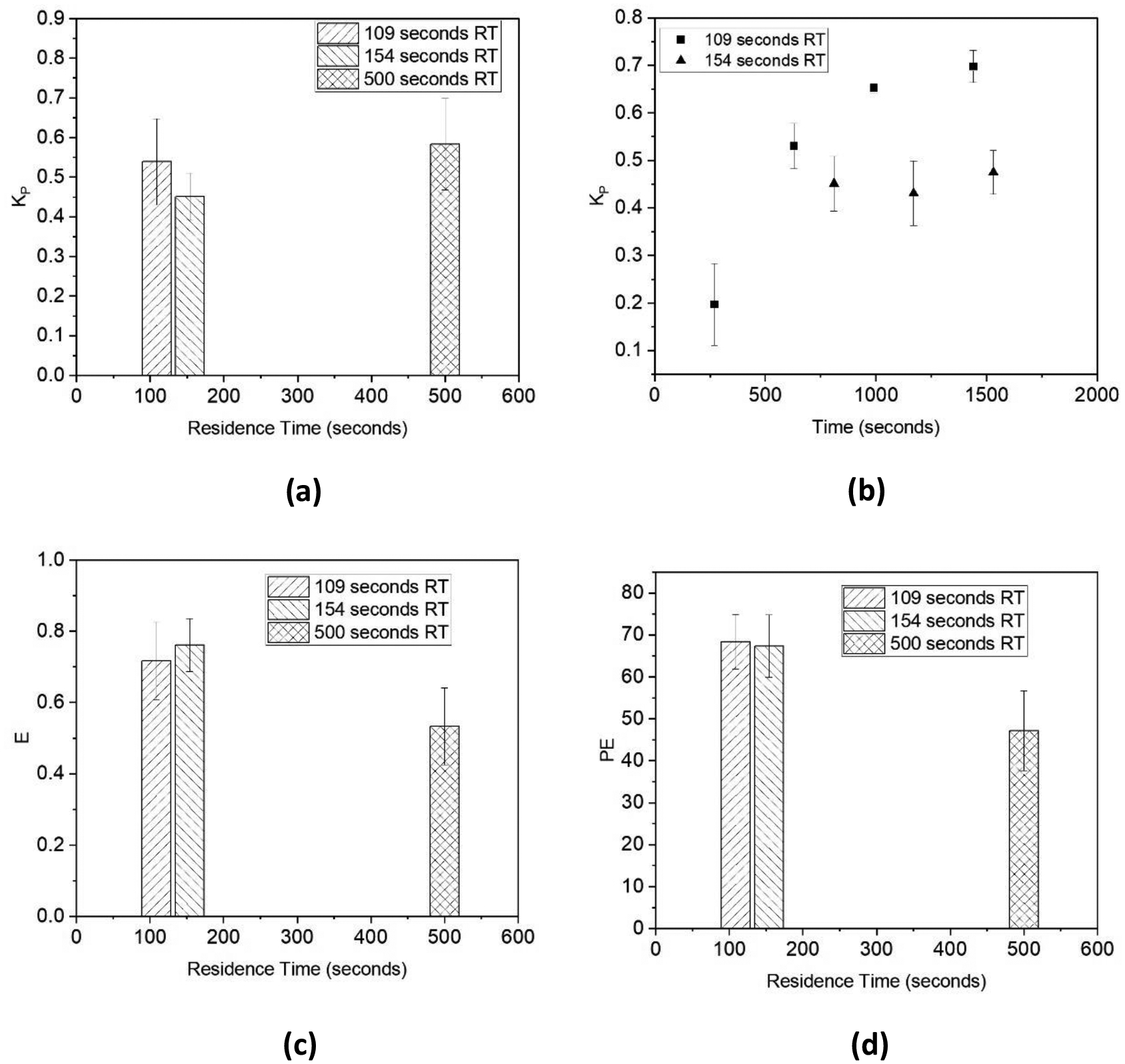
(a) Average partition coefficient vs. residence time (RT); (b) Partition coefficient of Exp. 1 with 154 seconds RT; (c) Average E vs. RT; and (d) average PE vs. RT
Extraction efficiency (E) is defined as a measure of how close the flow system is to equilibrium concentrations and is calculated using Eq. 10 [33]. Percent extraction, PE, of ISO into water was determined by Eq. 10.
| (9) |
| (10) |
Longer residence times seem more likely to result in higher extraction efficiency; however, Figure 10c suggests that at longer residence times extraction efficiency decreases. This phenomena has been shown by other researchers [33,49], who found that slug flow velocity had an inverse relationship with E.
Figure 11 displays time course plots for PE and E. The first three sample collections were not used in steady-state determination and can be attributed to startup. After 540 seconds the system appeared to approach steady-state operation as seen in Figure 11b. After large changes in the initial time points for both partition coefficient and extraction efficiency, later time points show decreased differences as the process appears to begin approaching a steady-state.
Figure 11:

(a) Variation of E and time and (b) PE with time
Between experimental conditions, the PE varied for both residence times shown, however, the residence time of 154 seconds yielded higher percent extraction. Since the difference in PE between residence times is not large, further experiments would be useful to provide further support of the claim that higher residence times yielding higher PE. In order to investigate the impact of longer residence times on extraction performace, a simulation-based approach was implemented.
3.3. Simulations of Various Residence times for Extraction using calculated KLa
In Figure 12a the comparison between the Matsuoka KLa method and experimental data are shown. The simulated concentration profiles based on 109 seconds provides an overprediction of the mass transfer coefficient when compared to the experimental data. In Figure 12b, the parity plot for the experimentally determined and model 1 predicted KLa.
Figure 12:
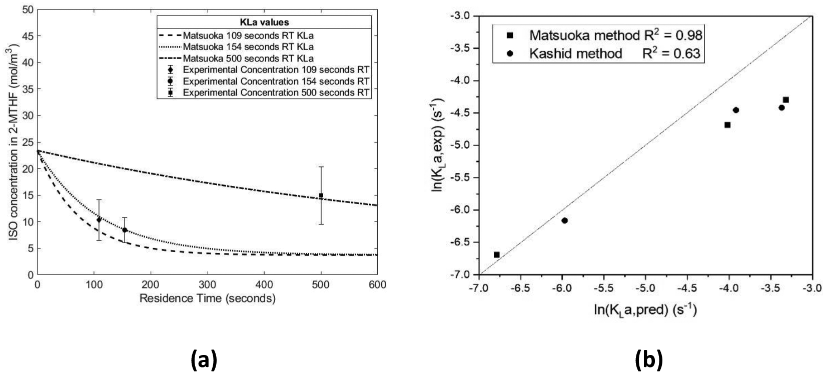
(a) Simulations of initial concentration of ISO vs. Residence Time; (b) Parity Plot for experimental and predicted KLa
The 154 and 500 seconds residence times provide an underprediction for the overall volumetric mass transfer coefficient when compared to the experimental concentration of ISO. This is in contrast to the experimental results obtained for batch extraction. The variation of the concentration of ISO is simulated as a function of the residence time, considering different initial concentrations Eq. 11 is a differential equation which models the change in concentration at various residence times. ODE45 in MatLab was used to solve the differential equation to provide time course concentration data for different implemented overall volumetric mass transfer coefficients. The authors sought to generate design spaces to better understand extraction performance in the operating space, so it was important to implement vectors with multiple initial ISO concentrations. ODE45 is better suited to complete these operations than ‘dsolve’, for example, which could also solve the differential equation.
| (11) |
Overall volumetric mass transfer coefficient (KLa) was determined by using the values obtained from the experimental results. Integrating Eq. 11 provides Eq. 12, and with some algebraic manipulation, Eq. 11 is formed from the initial condition that C1 is zero because E is zero at time equal zero.
| (12) |
| (13) |
Eq. 12 is a result of algebraic rearrangement for KLa.
| (14) |
For a more detailed explanation on the substitutions and derivation found in Eqs. 12 through 14, see Matsuoka and Mae [21].
The second volumetric mass transfer coefficient (KLa) experimental method, as seen in a study by Kashid et al. [33] was dependent on concentration measurements. The parameters along with 95% confidence interval (CI) values can be found in Table 4. E* is the equilibrium extraction efficiency that resulted from the 12-hour batch experiment.
Table 4:
Parameters for Simulations
| Parameter | Value (CI) | ||
|---|---|---|---|
| Matsuoka K L a [s −1 ] | 13.6×10⁻³ (10.1×10−3,17.2×10−3) |
9.194×10⁻³ (6.0 ×10−3,12.4×10−3) |
1.24×10⁻³ (1.22×10−3,1.26×10−3) |
| E | 71.7 (61.6,81.8) | 76.1 (63,80.4) | 53.33 (32.23,74.43) |
| E* | 88.3 (79.5,97.1) | 88.3 (79.5,97.1) | 88.3 (79.5,97.1) |
| t [s] | 109 | 154 | 500 |
| Kashid K L a [s −1 ] | 12×10−3 (9.50×10−3,14.6×10−3) |
11.6×10⁻³ (8.42×10−3,14.7×10−3) |
2.1×10⁻³
(0.40 ×10−3,3.81×10−3) |
| (15) |
3.4. Mass transfer coefficient model discrimination
In this investigation, two experimental methods for overall volumetric mass transfer coefficient were evaluated. Following the experimental method determination, a model was implemented to predict mass transfer and compare against experimental determination methods. The model by Kashid et al. [50] incorporates capillary number, Ca, and Reynold’s number, Re. Simulation-aided extractor design was then performed to compare against experimental findings and determine if there was any model mismatch. If the fluid properties can be measured, the implementation of additional models can be done without significant challenge; however, when information is limited, the method reported by Matsuoka and Mae provides a shortcut method to determine the overall mass transfer coefficient. To determine parameters β1 and β2, a nonlinear MatLab optimizer, ‘nlinfit’ was used, which also computed mean square error (MSE). The parameters and CI values are in Table 5. The compared methods report different magnitudes of error and the model fit to the KLa values determined by Matsuoka method provided the better fit for the experimental data. The differences in the fit of the models can be linked to the expressions to determine KLa as reported earlier.
Table 5:
Model Parameters
| MSE | |||
|---|---|---|---|
| Model 1: Fit for Matsuoka Method | −1.4083 (−1.8141, −1.0025) |
−4.651 (−6.0284, −3.2735) |
9.4513× 10⁻⁹ |
| Model 2: Fit for Kashid Method | −0.8983 (−5.7875,3.9908) |
−2.9184 (−19.3971,13.5603) |
3.9477× 10⁻⁶ |
| (16) |
In order to assess the fit of the two experimental methods for KLa determination with the respective models, a parity plot was created. Figure 12b shows that there is better agreement with the Matsuoka model and experimental KLa (R2 value of 0.93) than with the Kashid model and experimental KLa (R2 value of 0.65). While the models do not predict the exact values for the overall mass transfer coefficients, the trends are captured for the changes with respect to residence time.
Along with the parameter values that were estimated, a comparison between the goodness of fit and the two experimental methods are presented. Due to the lower MSE, model 1 for the Matsuoka experimental method was used for design space determination.
With the model and experimental KLa values determined, simulations could be carried out to see how well the models performed when compared to the experimental methods. In the case of the model 2 and Kashid experimental method, the model underpredicted the 109 seconds RT and over predicted the 154 and 500 seconds RT. In the case of the model 1 and Matsuoka experimental method, the model matches the experimental method well for 109 seconds RT and over predicts the 154 and 500 seconds RT.
4.5. Extraction Simulations and Design Space Determination
Following the parameter estimation, both the Kashid and Matsuoka experimental methods were compared to the models in Figure 13a and Figure 13b respectively. Comparing the simulation of the liquid-liquid extraction to the experimental data collected helped to determine if the models and experimental methods provided a good fit. In the case of the model and Kashid method, the KLa calculated in the 154 seconds residence time meets the error bounds of two of the three data points. The simulation of the concentration with the model and Matsuoka method experimental mass transfer coefficients show close matching for each residence time. Each of the simulations is within the error bounds of the experimental data points. The deviations with the Kashid and Matsuoka methods and the simulation models are likely due to the changing rates of mass transfer as a function of residence time. With the three residence times studied, there are large differences in the rates observed for the various residence times. In order to reduce the deviation between the simulations and experimental methods, ‘nlfit’ was implemented to minimize the error between the experimental KLa values and simulated KLa values.
Figure 13:
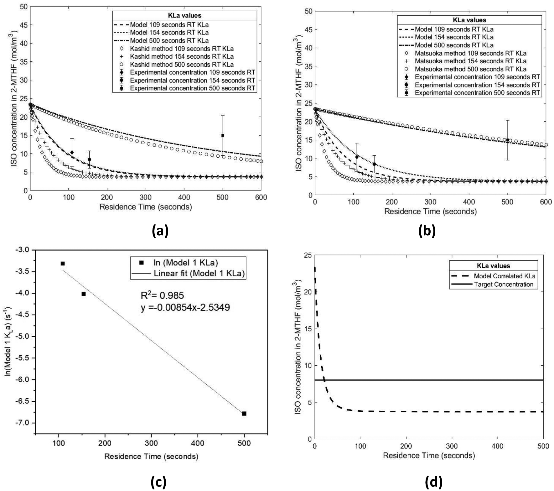
(a) Extraction simulations for model and Kashid method; (b) Extraction simulations for model and Matsuoka method; (c) Correlation between model ln(KLa) values and residence time; and (d) simulated extraction of predicted KLa values for target purity
In order to predict extraction performance at other residence times, a correlation was made between the model KLa values and the residence times for which they were calculated (Figure 13c). With the correlation overall mass transfer coefficients could be predicted as a function of the residence time. The simulation results were used to determine the residence time needed to achieve the target ISO concentration of 8 mol/m3 (Figure 13d). The target ISO concentration was determined by summation of the target threshold of 40 μg daily intake from guidance from PhRMA on daily exposure for 1–3 months for a total of 42 days [27]. Since Lomustine is prescribed as a single dose in a six week time span, this option seemed to be appropriate [38]. The simulation shows the target ISO concentration is met in 22 seconds.
After obtaining overall volumetric mass transfer coefficients using both the Kashid and Matsuoka methods, varying the initial concentration of ISO in each case showed the impact of initial concentration on the extraction design space. In Figure 14 the Matsuoka experimentally determined KLa values and modeled KLa values were used to simulate ISO extraction with respect to residence time at various initial ISO concentrations. For the KLa values that were the lowest (Figure 14e and Figure 14f) there was a much smaller region of the design space that met the target final concentration of ISO (denoted by black diagonal lines). At higher KLa values, the majority of the design space met the final target ISO concentration. It is important to consider which of these cases most accurately depicts what will happen within the experimental flow extraction set up. It is likely that KLa values that are moderate are better to predict the performance of the extraction platform when compared to the highest and lowest KLa. In efforts to gain a better fit of the experimental data, it was predicted that a model based KLa determination could be implemented. In the design spaces are shown side by side for the experimental and model prediction KLa values for the Matsuoka method.
Figure 14:

Design Space Plots for KLa (s−1) values of: (a) 13.6 ×10⁻³; (b) 36.0 ×10⁻³; (c) 9.194 ×10⁻³; (d) 18.0 ×10⁻³; (e) 1.24 ×10⁻³; (f) 1.129 ×10⁻³
With each of the KLa values that are simulated there are similar dynamics for the reduction of the ISO along the extractor length. Increased amounts of ISO would be indicative of a reaction step that was not fully completed in the first synthesis step for 1-(2-chloroethyl)-3-cyclohexylurea. At larger initial concentrations, the extractor length needed to achieve the target purity increases.
From the residence time (τl), an extractor length (l) can be determined assuming the constant diameter (d) of the tubular extractor. Simulations can also be extended to determine the impact of changes in initial concentration on the final extraction outcomes.
In an effort to capture the changing dynamics of the extraction, residence time dependent KLa was implemented (Eq.17). A substitution for KLa then yields Eq. 18.
| (17) |
| (18) |
The equation was solved using ODE45, which allowed for initial ISO concentrations to be simulated simultaneously to generate a design space. The resulting design space in Figure 15a is for the continuous extraction with the residence time dependent KLa values. In Figure 15b, the design space was generated with the fluid property dependent model KLa values. With all of the necessary components determined for the model implementation, design space plots could be generated based on the fluid property model in Eq. 16. In Figure 15a, the design space is displayed for the residence time dependent KLa values. For example, with an initial concentration of 20 mol/m3, the target concentration of ISO is predicted to be achieved after 20 seconds. For the case of the fluid property model KLa modeling, in Figure 15b, for the same initial condition of 25 mol/m3 the target concentration of 8 mol/m3 is achieved after 40 seconds. With model predicted design space, the target concentrations of ISO are predicted at longer residence times than the experimentally determined design space. Overall, the model-based approach provides conservative predictions for ISO extraction for the continuous extraction platform.
Figure 15:

Design Spaces for 600 second with (a) Residence Time Dependent KLa and (b) Fluid Property Model KLa
5. Conclusions
In this study various aspects of the extraction of ISO were explored including solvent selection, batch and continuous experimental work, parameter estimation, and simulation for design space generation. The data collected from the 12-hour batch experiment indicated concentration values in the organic phase that were much lower than those achieved in short residence times in the continuous extraction platform. Maximum extraction efficiency of 77% and percent extraction of ISO of 69% were achieved in flow on the continuous extraction platform. Through mathematical modeling approaches, models were fit to experimentally determined KLa values ranging from 1.29× 10⁻³ - 32.0× 10⁻³ s−1. The models enable the ability to use predicted mass transfer from fluid property values. A correlation between residence time and mass transfer coefficients allowed the estimation of extraction performance beyond the three residence times studied experimentally in this work. Additionally, a simulation-based approach was implemented to simulate the residence time to reach equilibrium concentrations in the organic phase and design an extractor to meet desired impurity concentration. Predictions for increased extraction with increased residence time aligns with the experimental results that showed some increases in the PE. This paper details the design, simulation, and construction of the continuous liquid-liquid extraction of ISO. The design and successful operation of the continuous extraction and separation platform was demonstrated for the first time for the extraction of ISO in 2-methyl tetrahydrofuran. From the small-scale extraction experiments, overall volumetric mass transfer coefficients were determined for modeling extraction design to use for predicting extraction operating conditions. Future experimental work can be conducted with longer residence times and exploring the impact of temperature on the trends predicted by the simulations.
Figure 9:

(a) Weber number, (b) Capillary number, (c) Reynold’s number, and (d) Pressure drop
Table 6:
Summary of Overall Mass Transfer Coefficients
| Residence Time (seconds) | Model 1 KLa | Experimental KLa (Matsuoka method) | Model 2 KLa | Experimental KLa (Kashid method) |
|---|---|---|---|---|
| 109 | 36.0×10⁻³ (35.0×10−3,38.0×10−3) |
13.6×10⁻³ (10.1×10−3,17.2×10−3) |
34.5×10⁻³ (15.9×10⁻³, 75.1×10⁻³) |
12.03×10⁻³ (9.495×10−3,14.6×10−3) |
| 154 | 18.0×10⁻³ (16.1×10−3,19.0×10−3) |
9.19×10⁻³ (6.0 ×10−3,12.4×10−3) |
19.93×10⁻³ (10.6×10−3,37.4×10−3) |
11.6×10⁻³
(8.42×10−3,14.7×10−3) |
| 500 | 1.13×10⁻³ (0.59×10−3,2.16×10−3) |
1.24×10⁻³ (1.22×10−3,1.26×10−3) |
2.56×10⁻³ (1×10⁻⁶, 4.477) |
2.1×10⁻³
(0.4×10−3,3.8×10−3) |
Acknowledgements
This study was supported by the U.S. Food and Drug Administration through grant U01FD006738.The views expressed by the authors do not necessarily reflect the official policies of the Department of Health and Human Services; nor does any mention of trade names, commercial practices, or organization imply endorsement by the United States Government. A special acknowledgement is for Professor David H. Thompson, who provided the HPLC system for the data collection and processing. The authors declare no financial conflicts of interest.
List of Symbols
- a
Area for mass transfer (m2)
- C
Concentration of ISO (mol/m3)
Integration constant
- CA,aq
Concentration of species A in aqueous phase (mol/m3)
- CA,org
Concentration of species A in organic phase (mol/m3)
Concentration of ISO in the organic phase entering the extractor (mol/m3)
Concentration of ISO in the organic phase leaving the extractor (mol/m3)
Concentration of ISO in the organic phase (mol/m3)
Concentration of ISO in the organic phase (mol/m3)
- Ca
Capillary number
- D
Tube diameter (m)
- E
Extraction efficiency
Equilibrium extraction efficiency
- Ecoh
Cohesive Energy (J/mol)
- KLa
Volumetric mass transfer coefficient (s−1)
- KP,A
Partition coefficient of species A
- KP,Theory
Partition coefficient calculation using solubility parameters
- l
Tubing length (m)
- Lc
Channel length (m)
- Lu
Slug unit length (m)
- P
Density (kg/m3)
- r
Tubing radius (m)
- R
Universal gas constant (J/mol·K)
- Re
Reynold’s number
- t
Residence Time (s)
- T
Temperature (K)
- U
Velocity (m/s)
- Umix
Velocity of solvent mixture (m/s)
- V
Extractor volume (m3)
Volumetric flow rate (m3/s)
- Vm
Molar volume (m3/mol)
- Vsep
Separator volume (m3)
- We
Weber number
- δ ISO
Solubility parameter for ISO
- δ 1
Solubility parameter for solvent 1
- δ 2
Solubility parameter for solvent 2
- δ 2-MTHF
Solubility parameter for 2-MTHF (MPa0.5)
- δ Heptane
Solubility parameter for Heptane (MPa0.5)
- δ Hexane
Solubility parameter for Hexane (MPa0.5)
- δ
Film thickness (m)
- ΔP
Pressure drop (kPa)
- E
Dispersed phase fraction
- μc
Viscosity of continuous phase (Pa·s)
- μd
Viscosity of dispersed phase (Pa·s)
- Σ
Surface tension (N/m)
- τl
Residence time (s)
- β1
Volumetric mass transfer coefficient model parameter 1
- β2
Volumetric mass transfer coefficient model parameter 2
- CHA
Cyclohexylamine
- DCM
Dichloromethane
- CI
Confidence Interval
- ISO
2-chloroethyl isocyanate
- 2-MTHF
2-methyl tetrahydrofuran
- INT
1-(2-chlroethyl)-3-cyclohexylurea
- PE
Percent Extraction
- PI
Process Intensification
- RT
Residence Time
- THF
Tetrahydrofuran
Footnotes
The authors declare no competing financial interest.
References
- [1].Siegel RL, Miller KD, Fuchs HE, Jemal A, Cancer statistics, 2022, CA: A Cancer Journal for Clinicians 72 (2022) 7–33. 10.3322/caac.21708. [DOI] [PubMed] [Google Scholar]
- [2].Jaman Z, Sobreira TJP, Mufti A, Ferreira CR, Cooks RG, Thompson DH, Rapid On-Demand Synthesis of Lomustine under Continuous Flow Conditions, Org. Process Res. Dev 23 (2019) 334–341. 10.1021/acs.oprd.8b00387. [DOI] [Google Scholar]
- [3].Delanghe S, Delanghe JR, Speeckaert R, Van Biesen W, Speeckaert MM, Mechanisms and consequences of carbamoylation, Nat Rev Nephrol 13 (2017) 580–593. 10.1038/nrneph.2017.103. [DOI] [PubMed] [Google Scholar]
- [4].Chakkath T, Lavergne S, Fan TM, Bunick D, Dirikolu L, Alkylation and Carbamylation Effects of Lomustine and Its Major Metabolites and MGMT Expression in Canine Cells, Veterinary Sciences 2 (2015) 52–68. 10.3390/vetsci2020052. [DOI] [PMC free article] [PubMed] [Google Scholar]
- [5].Kann HE Jr., Kohn KW, Lyles JM, Inhibition of DNA Repair by the 1,3-Bis(2-chloroethyl)-1-nitrosourea Breakdown Product, 2-Chloroethyl Isocyanate, Cancer Research 34 (1974) 398–402. [PubMed] [Google Scholar]
- [6].Yang Y, Tjia R, Process modeling and optimization of batch fractional distillation to increase throughput and yield in manufacture of active pharmaceutical ingredient (API), Computers & Chemical Engineering 34 (2010) 1030–1035. 10.1016/j.compchemeng.2010.03.019. [DOI] [Google Scholar]
- [7].Johnson MD, May SA, Calvin JR, Remacle J, Stout JR, Diseroad WD, Zaborenko N, Haeberle BD, Sun W-M, Miller MT, Brennan J, Development and Scale-Up of a Continuous, High-Pressure, Asymmetric Hydrogenation Reaction, Workup, and Isolation, Org. Process Res. Dev 16 (2012) 1017–1038. 10.1021/op200362h. [DOI] [Google Scholar]
- [8].Cole KP, Groh JM, Johnson MD, Burcham CL, Campbell BM, Diseroad WD, Heller MR, Howell JR, Kallman NJ, Koenig TM, May SA, Miller RD, Mitchell D, Myers DP, Myers SS, Phillips JL, Polster CS, White TD, Cashman J, Hurley D, Moylan R, Sheehan P, Spencer RD, Desmond K, Desmond P, Gowran O, Kilogram-scale prexasertib monolactate monohydrate synthesis under continuous-flow CGMP conditions, Science 356 (2017) 1144–1150. 10.1126/science.aan0745. [DOI] [PubMed] [Google Scholar]
- [9].Nașcu I, Diangelakis NA, Pistikopoulos EN, Multi-parametric Model Predictive Control Strategies for Evaporation Processes in Pharmaceutical Industries, in: Montastruc L, Negny S (Eds.), Computer Aided Chemical Engineering, Elsevier, 2022: pp. 1159–1164. 10.1016/B978-0-323-95879-0.50194-6. [DOI] [Google Scholar]
- [10].Nagy ZK, Fujiwara M, Woo XY, Braatz RD, Determination of the Kinetic Parameters for the Crystallization of Paracetamol from Water Using Metastable Zone Width Experiments, Ind. Eng. Chem. Res 47 (2008) 1245–1252. 10.1021/ie060637c. [DOI] [Google Scholar]
- [11].Yang Y, Song L, Nagy ZK, Automated Direct Nucleation Control in Continuous Mixed Suspension Mixed Product Removal Cooling Crystallization, Crystal Growth & Design 15 (2015) 5839–5848. 10.1021/acs.cgd.5b01219. [DOI] [Google Scholar]
- [12].Powell KA, Saleemi AN, Rielly CD, Nagy ZK, Monitoring Continuous Crystallization of Paracetamol in the Presence of an Additive Using an Integrated PAT Array and Multivariate Methods, Org. Process Res. Dev 20 (2016) 626–636. 10.1021/acs.oprd.5b00373. [DOI] [Google Scholar]
- [13].Diab S, Raiyat M, D. I. Gerogiorgis, Flow synthesis kinetics for lomustine, an anti-cancer active pharmaceutical ingredient, Reaction Chemistry & Engineering 6 (2021) 1819–1828. 10.1039/D1RE00184A. [DOI] [Google Scholar]
- [14].Bédard A-C, Longstreet AR, Britton J, Wang Y, Moriguchi H, Hicklin RW, Green WH, Jamison TF, Minimizing E-factor in the continuous-flow synthesis of diazepam and atropine, Bioorganic & Medicinal Chemistry 25 (2017) 6233–6241. 10.1016/j.bmc.2017.02.002. [DOI] [PubMed] [Google Scholar]
- [15].Mestmäcker F, Schmidt A, Huter M, Sixt M, Strube J, Systematic and Model-Assisted Process Design for the Extraction and Purification of Artemisinin from Artemisia annua L.—Part III: Chromatographic Purification, Processes 6 (2018) 180. 10.3390/pr6100180. [DOI] [Google Scholar]
- [16].Müller E, Berger R, Blass E, Sluyts D, Pfennig A, Liquid–Liquid Extraction, in: Ullmann’s Encyclopedia of Industrial Chemistry, John Wiley & Sons, Ltd, 2008. 10.1002/14356007.b03_06.pub2. [DOI] [Google Scholar]
- [17].Zhu Z, Bai W, Xu Y, Gong H, Wang Y, Xu D, Gao J, Liquid-liquid extraction of methanol from its mixtures with hexane using three imidazolium-based ionic liquids, The Journal of Chemical Thermodynamics 138 (2019) 189–195. 10.1016/j.jct.2019.06.024. [DOI] [Google Scholar]
- [18].Adamo A, Beingessner RL, Behnam M, Chen J, Jamison TF, Jensen KF, Monbaliu J-CM, Myerson AS, Revalor EM, Snead DR, Stelzer T, Weeranoppanant N, Wong SY, Zhang P, On-demand continuous-flow production of pharmaceuticals in a compact, reconfigurable system, Science 352 (2016) 61–67. 10.1126/science.aaf1337. [DOI] [PubMed] [Google Scholar]
- [19].Weeranoppanant N, Adamo A, Saparbaiuly G, Rose E, Fleury C, Schenkel B, Jensen KF, Design of Multistage Counter-Current Liquid–Liquid Extraction for Small-Scale Applications, Ind. Eng. Chem. Res 56 (2017) 4095–4103. 10.1021/acs.iecr.7b00434. [DOI] [Google Scholar]
- [20].Sahu A, Vir AB, Molleti LNS, Ramji S, Pushpavanam S, Comparison of liquid-liquid extraction in batch systems and micro-channels, Chemical Engineering and Processing: Process Intensification 104 (2016) 190–200. 10.1016/j.cep.2016.03.010. [DOI] [Google Scholar]
- [21].Matsuoka A, Mae K, Design strategy of a microchannel device for liquid–liquid extraction based on the relationship between mass transfer rate and two-phase flow pattern, Chemical Engineering and Processing - Process Intensification 160 (2021) 108297. 10.1016/j.cep.2021.108297. [DOI] [Google Scholar]
- [22].Singh KK, Renjith AU, Shenoy KT, Liquid–liquid extraction in microchannels and conventional stage-wise extractors: A comparative study, Chemical Engineering and Processing: Process Intensification 98 (2015) 95–105. 10.1016/j.cep.2015.10.013. [DOI] [Google Scholar]
- [23].Reay D, Ramshaw C, Harvey A, eds., Chapter 2 - Process intensification – an overview, in: Process Intensification, Butterworth-Heinemann, Oxford, 2008: pp. 21–45. 10.1016/B978-0-7506-8941-0.00003-1. [DOI] [Google Scholar]
- [24].Zhang P, Weeranoppanant N, Thomas DA, Tahara K, Stelzer T, Russell MG, O’Mahony M, Myerson AS, Lin H, Kelly LP, Jensen KF, Jamison TF, Dai C, Cui Y, Briggs N, Beingessner RL, Adamo A, Advanced Continuous Flow Platform for On-Demand Pharmaceutical Manufacturing, Chemistry – A European Journal 24 (2018) 2776–2784. 10.1002/chem.201706004. [DOI] [PubMed] [Google Scholar]
- [25].ICH Expert Working Group, Q8(R2) Pharmaceutical Development, (2009). https://www.fda.gov/regulatory-information/search-fda-guidance-documents/q8r2-pharmaceutical-development.
- [26].Delaney EJ, An impact analysis of the application of the threshold of toxicological concern concept to pharmaceuticals, Regulatory Toxicology and Pharmacology 49 (2007) 107–124. 10.1016/j.yrtph.2007.06.008. [DOI] [PubMed] [Google Scholar]
- [27].Müller L, Mauthe RJ, Riley CM, Andino MM, Antonis DD, Beels C, DeGeorge J, De Knaep AGM, Ellison D, Fagerland JA, Frank R, Fritschel B, Galloway S, Harpur E, Humfrey CDN, Jacks AS, Jagota N, Mackinnon J, Mohan G, Ness DK, O’Donovan MR, Smith MD, Vudathala G, Yotti L, A rationale for determining, testing, and controlling specific impurities in pharmaceuticals that possess potential for genotoxicity, Regulatory Toxicology and Pharmacology 44 (2006) 198–211. 10.1016/j.yrtph.2005.12.001. [DOI] [PubMed] [Google Scholar]
- [28].ICH Expert Working Group, Q9 Quality Risk Management, (2006). https://www.fda.gov/regulatory-information/search-fda-guidance-documents/q9-quality-risk-management.
- [29].ICH Expert Working Group, Q10 Pharmaceutical Quality System, (2009). https://www.fda.gov/regulatory-information/search-fda-guidance-documents/q10-pharmaceutical-quality-system.
- [30].Grom M, Stavber G, Drnovšek P, Likozar B, Modelling chemical kinetics of a complex reaction network of active pharmaceutical ingredient (API) synthesis with process optimization for benzazepine heterocyclic compound, Chemical Engineering Journal 283 (2016) 703–716. 10.1016/j.cej.2015.08.008. [DOI] [Google Scholar]
- [31].Armstrong CT, Pritchard CQ, Cook DW, Ibrahim M, Desai BK, Whitham PJ, Marquardt BJ, Chen Y, Zoueu JT, Bortner MJ, Roper TD, Continuous flow synthesis of a pharmaceutical intermediate: a computational fluid dynamics approach, Reaction Chemistry & Engineering 4 (2019) 634–642. 10.1039/C8RE00252E. [DOI] [PMC free article] [PubMed] [Google Scholar]
- [32].Fath V, Lau P, Greve C, Kockmann N, Röder T, Efficient Kinetic Data Acquisition and Model Prediction: Continuous Flow Microreactors, Inline Fourier Transform Infrared Spectroscopy, and Self-Modeling Curve Resolution, Org. Process Res. Dev 24 (2020) 1955–1968. 10.1021/acs.oprd.0c00037. [DOI] [Google Scholar]
- [33].Kashid MN, Harshe YM, Agar DW, Liquid−Liquid Slug Flow in a Capillary: An Alternative to Suspended Drop or Film Contactors, Ind. Eng. Chem. Res 46 (2007) 8420–8430. 10.1021/ie070077x. [DOI] [Google Scholar]
- [34].Diab S, Gerogiorgis DI, Technoeconomic Mixed Integer Nonlinear Programming (MINLP) optimization for design of Liquid-Liquid Extraction (LLE) cascades in continuous pharmaceutical manufacturing of atropine, AIChE Journal 65 (2019) e16738. 10.1002/aic.16738. [DOI] [Google Scholar]
- [35].Szilágyi B, Nagy ZK, Aspect Ratio Distribution and Chord Length Distribution Driven Modeling of Crystallization of Two-Dimensional Crystals for Real-Time Model-Based Applications, Crystal Growth & Design 18 (2018) 5311–5321. 10.1021/acs.cgd.8b00758. [DOI] [Google Scholar]
- [36].Szilágyi B, Eren A, Quon JL, Papageorgiou CD, Nagy ZK, Monitoring and digital design of the cooling crystallization of a high-aspect ratio anticancer drug using a two-dimensional population balance model, Chemical Engineering Science 257 (2022) 117700. 10.1016/j.ces.2022.117700. [DOI] [Google Scholar]
- [37].Rasche ML, Jiang M, Braatz RD, Mathematical modeling and optimal design of multi-stage slug-flow crystallization, Computers & Chemical Engineering 95 (2016) 240–248. 10.1016/j.compchemeng.2016.09.010. [DOI] [Google Scholar]
- [38].Weiss RB, Issell BF, The nitrosoureas: carmustine (BCNU) and lomustine (CCNU), Cancer Treatment Reviews 9 (1982) 313–330. 10.1016/S0305-7372(82)80043-1. [DOI] [PubMed] [Google Scholar]
- [39].Taylor JW, Armstrong T, Kim AH, Venere M, Acquaye A, Schrag D, Wen PY, The lomustine crisis: awareness and impact of the 1500% price hike, Neuro-Oncology 21 (2019) 1–3. 10.1093/neuonc/noy189. [DOI] [PMC free article] [PubMed] [Google Scholar]
- [40].Aycock DF, Solvent Applications of 2-Methyltetrahydrofuran in Organometallic and Biphasic Reactions, Org. Process Res. Dev 11 (2007) 156–159. 10.1021/op060155c. [DOI] [Google Scholar]
- [41].Scott JL, Sneddon HF, Green Solvents, in: Green Techniques for Organic Synthesis and Medicinal Chemistry, John Wiley & Sons, Ltd, 2018: pp. 21–42. 10.1002/9781119288152.ch2. [DOI] [Google Scholar]
- [42].Hansen CM, Hansen solubility parameters: a user’s handbook, CRC Press, Boca Raton, Fla., 2000. [Google Scholar]
- [43].Donahue DJ, Bartell FE, The Boundary Tension at Water-Organic Liquid Interfaces, J. Phys. Chem 56 (1952) 480–484. 10.1021/j150496a016. [DOI] [Google Scholar]
- [44].Içten E, Maloney AJ, Beaver MG, Shen DE, Zhu X, Graham LR, Robinson JA, Huggins S, Allian A, Hart R, Walker SD, Rolandi P, Braatz RD, A Virtual Plant for Integrated Continuous Manufacturing of a Carfilzomib Drug Substance Intermediate, Part 1: CDI-Promoted Amide Bond Formation, Org. Process Res. Dev 24 (2020) 1861–1875. 10.1021/acs.oprd.0c00187. [DOI] [Google Scholar]
- [45].Içten E, Maloney AJ, Beaver MG, Zhu X, Shen DE, Robinson JA, Parsons AT, Allian A, Huggins S, Hart R, Rolandi P, Walker SD, Braatz RD, A Virtual Plant for Integrated Continuous Manufacturing of a Carfilzomib Drug Substance Intermediate, Part 2: Enone Synthesis via a Barbier-Type Grignard Process, Org. Process Res. Dev 24 (2020) 1876–1890. 10.1021/acs.oprd.0c00188. [DOI] [Google Scholar]
- [46].Maloney AJ, Içten E, Capellades G, Beaver MG, Zhu X, Graham LR, Brown DB, Griffin DJ, Sangodkar R, Allian A, Huggins S, Hart R, Rolandi P, Walker SD, Braatz RD, A Virtual Plant for Integrated Continuous Manufacturing of a Carfilzomib Drug Substance Intermediate, Part 3: Manganese-Catalyzed Asymmetric Epoxidation, Crystallization, and Filtration, Org. Process Res. Dev 24 (2020) 1891–1908. 10.1021/acs.oprd.0c00189. [DOI] [Google Scholar]
- [47].Van krevelen DW, CHAPTER 7 - COHESIVE PROPERTIES AND SOLUBILITY, in: Van krevelen DW (Ed.), Properties of Polymers (Third Edition), Elsevier, Amsterdam, 1997: pp. 189–225. 10.1016/B978-0-444-82877-4.50014-7. [DOI] [Google Scholar]
- [48].Jovanović J, Zhou W, Rebrov EV, Nijhuis TA, Hessel V, Schouten JC, Liquid–liquid slug flow: Hydrodynamics and pressure drop, Chemical Engineering Science 66 (2011) 42–54. 10.1016/j.ces.2010.09.040. [DOI] [Google Scholar]
- [49].Vural Gürsel I, Kurt SK, Aalders J, Wang Q, Noël T, Nigam KDP, Kockmann N, Hessel V, Utilization of milli-scale coiled flow inverter in combination with phase separator for continuous flow liquid–liquid extraction processes, Chemical Engineering Journal 283 (2016) 855–868. 10.1016/j.cej.2015.08.028. [DOI] [Google Scholar]
- [50].Kashid MN, Gupta A, Renken A, Kiwi-Minsker L, Numbering-up and mass transfer studies of liquid–liquid two-phase microstructured reactors, Chemical Engineering Journal 158 (2010) 233–240. 10.1016/j.cej.2010.01.020. [DOI] [Google Scholar]