A robust model training strategy using hard negative mining in a weakly labeled dataset for lymphatic invasion in gastric cancer

Abstract

Gastric cancer is a significant public health concern, emphasizing the need for accurate evaluation of lymphatic invasion (LI) for determining prognosis and treatment options. However, this task is time‐consuming, labor‐intensive, and prone to intra‐ and interobserver variability. Furthermore, the scarcity of annotated data presents a challenge, particularly in the field of digital pathology. Therefore, there is a demand for an accurate and objective method to detect LI using a small dataset, benefiting pathologists. In this study, we trained convolutional neural networks to classify LI using a four‐step training process: (1) weak model training, (2) identification of false positives, (3) hard negative mining in a weakly labeled dataset, and (4) strong model training. To overcome the lack of annotated datasets, we applied a hard negative mining approach in a weakly labeled dataset, which contained only final diagnostic information, resembling the typical data found in hospital databases, and improved classification performance. Ablation studies were performed to simulate the lack of datasets and severely unbalanced datasets, further confirming the effectiveness of our proposed approach. Notably, our results demonstrated that, despite the small number of annotated datasets, efficient training was achievable, with the potential to extend to other image classification approaches used in medicine.

Introduction

Gastric cancer is a major global public health concern, with a reported incidence of more than 1 million new cases and 769,000 deaths in 2020 alone [1]. Specific regions such as East Asia, Eastern Europe, and South America are particularly affected by gastric cancer and its complications. Lymphatic invasion (LI) plays a crucial role in the prognosis and treatment of gastric cancer. As per the invasion–metastasis cascade theory, LI occurs when tumor cells enter the lymphatic system, which is a key event during cancer cell dissemination. LI is associated with a poor prognosis and an increased risk of recurrence, making it an important factor to consider in treatment decisions [2, 3, 4, 5, 6, 7]. However, accurate evaluation of the presence of LI remains a challenge for pathologists because of the labor‐intensive and time‐consuming nature of the task and the potential for intraobserver and interobserver variability.

Recently, computational pathology has made significant advancements in the field by enabling high‐resolution imaging of tissue specimens using whole slide images (WSIs). This technology allows the digitization of slide images, which can then be stored and analyzed using deep learning‐based artificial intelligence (AI) algorithms. These algorithms can be used to classify and detect pathological features with a high degree of accuracy and efficiency [8, 9, 10, 11]. However, the detection of LI using digital pathology remains challenging for several reasons: (1) complex patterns, (2) variability of the lymphatic system, and (3) scarcity of LI regions.

Previous studies attempted to detect LI using segmentation models. Ghosh et al [12] used a segmentation model to detect LI foci in testicular cancer, whereas Chen et al [13] attempted to detect LI in breast cancer using a similar approach. However, these studies were limited by the scarcity of labeled data and the potential for intra‐ and interobserver variability, which could affect the accuracy and robustness of the models. To address these challenges, we propose a classification‐based approach for LI detection using digital pathology. This approach is simpler and easier to train than the segmentation‐based approaches.

Although classification‐based approaches offer a simpler and more efficient way of detecting LI in digital pathology, they require a large number of annotated datasets for effective training. This requirement presents a challenge in medical image assessment, in which the collection and annotation of data can be costly and time‐consuming. Several approaches have been proposed to address this issue, including unsupervised, active, and semisupervised learning. Semisupervised learning is a powerful approach that utilizes both labeled and unlabeled data to train a model. Notably, this approach maximizes the use of weakly labeled datasets, thereby improving the performance of deep learning‐based AI algorithms in medical diagnosis systems.

Hard negative mining is a technique employed in semisupervised learning to improve the performance of deep learning models in object detection and classification tasks, as demonstrated in numerous studies [8, 9, 10, 11, 14, 15]. This approach involves the identification and selection of challenging negative samples incorrectly classified by the current model; thereafter, these samples are employed to train the model, thereby yielding a robust model. Hard negative mining improves the performance of deep learning models for various medical imaging applications, including the classification of pulmonary nodules [16, 17, 18], diagnosis of prostate cancer [19, 20], and analysis of skin lesions [21, 22]. Moreover, this method mitigates false positives, enhances sensitivity, and improves the overall accuracy of deep learning models. Furthermore, the proposed method demonstrates the capacity to train models that exhibit increased robustness in the face of class imbalance [23]. The application of hard negative mining has the potential to advance the creation of deep learning algorithms for various medical imaging applications.

This study aimed to evaluate the potential of deep learning algorithms for detecting and classifying LI in gastric cancer histopathology images. This study aimed to develop a robust model that can cope with a small‐sized and/or class‐imbalanced annotated dataset. This was achieved by (1) developing a deep learning‐based model for detecting LI in gastric cancer histopathology images and (2) training a model based on hard negative mining, a semisupervised learning technique.

Materials and methods

Study populations

Patients who underwent stomach excision at Korea University Anam Hospital between March 2021 and February 2022 were included in the study. All patients underwent excision surgery, including total gastrectomy, subtotal gastrectomy, and endoscopic submucosal dissection with or without lymph node dissection. The 115 archived WSIs were obtained from 81 patients. Clinicopathological factors, including age, sex, histological diagnosis, and other pathological features, were retrieved from the pathology reports (Table 1). Histological diagnosis was performed in accordance with the 2019 WHO classification of tumors of the digestive system (fifth edition), and TNM staging was performed in accordance with the eighth edition of the American Joint Committee on Cancer staging system [3, 24].

Table 1.

Clinicopathological factors of the 81 patients

Variable	Hard‐labeled dataset	Weakly labeled dataset	p value
	N = 54, n (%)	N = 27, n (%)
Sex
Male	40 (74.07)	18 (66.67)	0.486*
Female	14 (25.93)	9 (33.33)
Age	65.26 ± 11.29	69.83 ± 11.92	0.102 †
Procedure
Endoscopic submucosal dissection	7 (12.96)	13 (48.15)	0.001*
Subtotal gastrectomy	37 (68.52)	13 (48.15)
Total gastrectomy	10 (18.52)	1 (3.70)
Histologic type
Tubular adenocarcinoma, well differentiated	4 (7.41)	13 (48.15)	<0.001*
Tubular adenocarcinoma, moderately differentiated	30 (55.56)	7 (25.93)
Tubular adenocarcinoma, poorly differentiated	7 (12.96)	1 (3.70)
Poorly cohesive carcinoma	12 (22.22)	5 (18.52)
Carcinoma with lymphoid stroma	0 (0.00)	1 (3.70)
Hepatoid adenocarcinoma	1 (1.85)	0 (0.00)
Depth of invasion
Mucosal (pT1a)	3 (5.56)	19 (70.37)	<0.001*
Submucosal (pT1b)	18 (33.33)	4 (14.81)
Muscularis propria (pT2)	10 (18.52)	2 (3.70)
Subserosal connective tissue (pT3)	9 (16.67)	1 (3.70)
Serosa (pT4a)	12 (22.22)	1 (3.70)
Adjacent organ (pT4b)	2 (3.70)	–
Lymphatic invasion
Absence	–	27	–
Presence	54	–
Venous invasion
Absence	43 (79.63)	26 (96.30)	0.047*
Presence	11 (20.37)	1 (3.70)
Perineural invasion
Absence	28 (51.85)	23 (85.19)	0.003*
Presence	26 (48.15)	4 (14.81)
Lymph node status
Nx	7 (12.96)	13 (48.15)	<0.001*
N0	9 (16.67)	12 (44.44)
N1‐3	38 (70.37)	2 (7.41)

^*Chi‐square test.

^† Student's t‐test.

Dataset

Slide images were scanned using an Aperio AT2 digital slide scanner (Leica Biosystems, Wetzlar, Germany) with a ×20 objective (0.5 μm/pixel). The entire dataset was divided into two datasets: hard labeled and weakly labeled. All WSIs were from hematoxylin and eosin–stained slides. To accurately assess LI, only cases confirmed by D2‐40 immunohistochemical staining were included [25, 26]. This study was approved by the Institutional Review Board of Korea University Hospital (2023AN0039), and the requirement for informed consent was waived.

The hard‐labeled dataset consisted of 27 patients, and expert gastrointestinal pathologists, J. Sim and S. Ahn, confirmed that 48 WSIs corresponded to positive LI status. LI‐positive and LI‐negative regions are marked in Figure 1. Annotation was conducted using an open‐source platform, the automated slide analysis platform (Diagnostic Image Analysis Group, Nijmegen, The Netherlands). In total, 302 LI‐positive and 671 LI‐negative regions were annotated. As LI refers to tumor cells entering the lymphatic system, negative labels are assigned to lymphatic vessels without tumor cells. Patch images were generated using a standard digital pathology image analysis approach involving sampling from the WSI. The datasets were randomly shuffled at the WSI level in a 6:2:2 ratio for the training, validation, and test sets. The initial size of the patch images was 512 × 512 pixels with a ×5 objective setting (2 μm/pixel).

Figure 1.

A set of patch images representing LI‐positive and LI‐negative samples. The images depict (A, B) LI‐positive and (C, D) LI‐negative patches, respectively. The LI‐positive areas are highlighted with red boxes, while the LI‐negative areas are marked with green boxes. Note that the LI‐positive patch image may contain one or more LI‐positive areas, and the number of LI‐negative areas does not impact the classification. Conversely, the LI‐negative patch image should not contain any LI‐positive areas.

The weakly labeled dataset comprised 56 patients and 56 WISs whose final diagnosis of LI was negative. The dataset was referred to as weakly labeled because it contained only a final diagnosis label without annotations. Patch images were generated using the sliding‐window method without overlap, and one‐third of the total patch images were randomly sampled to reduce redundancy. The resolution of the patch images was consistent with that of the hard‐labeled dataset.

Model development

To develop a classification model for LI diagnosis, the ResNet 18 model that was pretrained on ImageNet weights was utilized. The binary cross‐entropy loss and Adam optimizer with a learning rate 1e−4 were utilized, with the learning rate controlled using a cosine annealing scheduler. During the training step, data augmentation techniques, such as geometric transformation, elastic deformation, blurring, and adjustments in brightness and contrast, were applied to the input patch images. Patch images were resized to 224 × 224‐pixel size for processing. After 30 epochs, the weights of the model with the minimum loss were selected as the final model parameters. To determine binary labels, a threshold of 0.1 was set. The model was developed using Python 3.9 and Pytorch 2.0.0 with automated half precision.

A conceptual diagram of LI classification using hard negative mining is shown in Figure 2. The model training process was initiated using a hard‐labeled dataset (weak model). After the initial training, false‐positive predictions were selected, and similar images were queried from the weakly labeled dataset. The number of N similar patch images was selected and added to the original training dataset to form an augmented dataset, which was then utilized to train a strong model.

Figure 2.

A schematic diagram of the weak–strong model training process with hard negative mining. The weak model was initially trained to utilize a hard‐labeled dataset annotated by human experts. False‐positive images, which the weak model struggled to accurately classify, were selected and similar images were queried from the weakly labeled dataset. The original training dataset was augmented with these queried images to train a stronger model.

Hard negative mining

In this study, a hard negative mining algorithm was used to improve a weakly supervised object detection model. The algorithm, presented in Algorithm 1, involves collecting false positives among the patch images misclassified by the weak model. The image features of these false‐positive patches were obtained using activation maps immediately before the classification head of the weak model.

Algorithm 1. Hard negative mining algorithm.

INPUT:

f(·): last hidden layer of the weak model

$x_{\text{false}}^i$: false positive of the weak model, $i=1,\dots ,N.$

$x_{\text{weakly}}^j$: weakly labeled dataset $j=1,\dots ,M$

$\alpha$: the number of data to query

OUTPUT:

$x_{\text{hard}}$: hard negative

For i = 1 to N do

Compute hidden state using $f\left(x_{\text{false}}^i\right)$

For j = 1 to M do

Compute hidden state using $f\left(x_{\text{weakly}}^j\right)$

Compute similarity score $S_{i,j}$ based on Equations (1) or (2)

End for

Select $\alpha$ of the most similar data in the $S_{i,j}$

Add data to $x_{\text{hard}}$

End for

Next, the features of all patch images in the weakly labeled dataset were computed. In this study, we employed L2 distance (Euclidean distance) and cosine similarity as the metrics for assessing similarity. It is noteworthy that alternative measures can be considered for this purpose. The L2 distance, represented by Equation (1), and the cosine similarity, expressed in Equation (2), were employed to calculate the similarity score $S_{i,j}$, where $x_i$ and $x_j$ denote the feature vectors corresponding to the false‐positive and weakly labeled patches, respectively.

$$S_{i,j}^{L2}=\sqrt{{\left(x_i-x_j\right)}^2}.$$ (1)

$$S_{i,j}^{\cos }=\frac{x_i·x_j}{‖x_i‖‖x_j‖}.$$ (2)

In this equation, $x_i$ and $x_j$ are elements of ${\mathcal{R}}^{d_{\text{model}}}$, where $d_{\text{model}}$ is the last hidden dimension of each weak model. Subscripts i and j correspond to individual data points. The α parameter, representing the number of samples similar to the query for each false‐positive patch, served as a hyperparameter that could be influencing the performance. In each experiment, in the absence of explicit specification of the alpha parameter, it was standardized to a value of 20. Similarly, if the query criteria were not specified, they were set to utilize the L2 distance.

Ablation study

To evaluate the efficacy of hard negative mining, we conducted experiments by perturbing the original training dataset in two ways. First, we perturbed only the positive labels under the assumption that the number of positive cases was limited, and randomly sampled 10%, 30%, 50%, and 70% of the positive labels. Second, we perturbed the entire dataset without considering labels and randomly sampled 10%, 30%, 50%, and 70% of the dataset. In this scenario, the entire dataset is assumed to be restricted. For each subset of the training dataset, we followed the same procedures involving weak model training, hard negative mining, and strong model training.

t‐distributed stochastic neighbor embedding and gradient‐weighted class activation mapping visualization

To visualize the high‐dimensional features of the model, we utilized t‐distributed stochastic neighbor embedding (t‐SNE) analysis. [27] The hyperparameters were set to 50 perplexities, and 500 perplexities were used in this analysis. In addition, to further visualize the areas of focus within the model, we applied gradient‐weighted class activation mapping (Grad‐CAM) to predict patch images. [28] The Grad‐CAM technique marked the focused area in red, allowing for the interpretation of the areas that were most critical in determining the model's final decision.

Statistical analysis

To evaluate prediction performance, several metrics were utilized, such as the area under the receiver operating characteristic (AUROC) curve, area under the precision‐recall curve (AUPRC), F1 score, sensitivity, and specificity. The F1 score is a metric that combines positive predictive value (precision) and sensitivity (recall) into a single value, providing a balanced measure of a model's performance, particularly useful in class imbalanced classification tasks; the equation is as follows:

$$F1\text{score}=2\times \frac{\text{precision}\times \text{recall}}{\text{precision}+\text{recall}}.$$ (3)

Results

Patient characteristics

The clinicopathological characteristics of the patients are summarized in Table 1. Patients' ages ranged from 35 to 95 years, with a mean age of 68.3 years. The study cohort consisted of 58 male patients and 23 female patients. Among the 81 gastric carcinoma cases, the most common histological type was tubular adenocarcinoma, which was well differentiated (17 cases, 21.0%), moderately differentiated (37 cases, 45.7%), and poorly differentiated (solid) (8 cases, 9.9%). The other histological types included 17 poorly cohesive carcinomas, including signet ring cell carcinoma (21.0%), 1 carcinoma with lymphoid stroma (1.2%), and 1 hepatoid adenocarcinoma (1.2%). The T stage comprised 22 patients with T1a, 22 with T1b, 12 with T2, 10 with T3, 13 with T4a, and 2 with T4b tumors. Of the 81 patients, 54 (66.7%) had LI, 12 (14.8%) had venous invasion, and 51 (63%) had perineural invasion. Forty (49.4%) patients had lymph node metastasis. Sex and age did not exhibit statistically significant differences between the hard‐labeled and weakly labeled datasets. However, the remaining variables, namely histological type (p < 0.001), depth of invasion (p < 0.001), venous invasion (p = 0.047), perineural invasion (p = 0.003), and lymph node status (p < 0.001), showed significant differences. Given that LI is associated with poor prognosis, it was reasonable to observe a higher presence of risk factors in the hard‐labeled dataset with LI.

LI classification performances

We evaluated the effectiveness of hard negative mining in improving the performance of classification models. The false‐positive patch images of the weak model and the queried hard negative patch images are depicted in Figure 3. The results obtained using the three randomly initialized models are summarized in Table 2 and Figure 4, indicating that the use of hard negative mining led to a significant improvement in classification. Irrespective of the chosen similarity measurements, namely L2 distance and cosine similarity, the classification performance of the hard model exhibited enhancements across all metrics except for the sensitivity of cosine similarity. Comparatively, the L2 distance‐based hard negative mining demonstrated superior performance compared with the cosine similarity‐based approach. Specifically, for L2 distance‐based hard negative mining, improvements were observed in AUROC (2.88%), AUPRC (2.17%), F1 (5.83%), sensitivity (6.39%), and specificity (4.72%).

Figure 3.

Sample false‐positive and hard negative patch images. In the upper row panels (A–D), the false positive instances are presented. These images exhibit blood vessels containing red blood cells, along with gland cells showing distortion caused by retraction artifact. In the lower row panels (E–H), the hard negative patch images are depicted. The selection of candidate images for hard negative mining was guided by feature similarity, resulting in the identification of hard negative samples that exhibited comparable patterns to the false‐positive samples (upper row panels).

Table 2.

Classification performances

Query criterion	Model	AUROC	AUPRC	F1 score	Sensitivity	Specificity
L2 distance	Weak	0.9465 (0.00)	0.9299 (0.02)	0.8821 (0.01)	0.8393 (0.02)	0.9012 (0.01)
	Strong	0.9738 (0.01)	0.9501 (0.01)	0.9334 (0.03)	0.8930 (0.03)	0.9437 (0.02)
	Delta	2.88%	2.17%	5.83%	6.39%	4.72%
Cosine similarity	Weak	0.9424 (0.02)	0.9324 (0.02)	0.8632 (0.02)	0.8502 (0.06)	0.8690 (0.05)
	Strong	0.9682 (0.01)	0.9496 (0.01)	0.9132 (0.01)	0.7910 (0.07)	0.9477 (0.01)
	Delta	2.74%	1.85%	5.79%	−6.97%	9.06%

The score is the average value of three random initialized models. The standard deviation is reported in brackets.

Figure 4.

Raider plot of classification performances. The results are presented in two panels for the perturbing condition, which includes the entire dataset and the positive label‐only condition. The left, middle, and right panels correspond to the AUROC, AUPRC, and F1 scores, respectively. The weak model's performance is indicated by the green color, while the strong model's performance is shown by the gray color. In each plot, the green area represents the weak model's performance, and the gray area represents the strong model's performance. It is noteworthy that the gray areas always cover the green areas, indicating that the strong model's performance surpasses that of the weak model in all three evaluation metrics.

In our setting, the strong model trained using hard negative mining with L2 distance‐based queried models exhibited notable classification performance on LI with values of 0.9738, 0.9501, 0.9334, 0.8930, and 0.9437 for AUROC, AUPRC, F1 score, sensitivity, and specificity, respectively.

Impact of the number of hard negative images, parameter α

The impact of hard negative mining exhibited a linear increase corresponding to the parameter α, as shown in Table 3. The enhancements in AUROC were 1.89% (α = 5), 2.55% (10), 2.88% (20), 3.59% (50), and 4.05% (100). Similarly, improvements in AUPRC were 1.16% (5), 2.41% (10), 2.17% (20), 2.32% (50), and 3.02% (100). This suggests that, by having adequate computational resources and a sufficient amount of weakly labeled datasets, increasing the alpha parameter has the potential to improve the performance of the model.

Table 3.

Influence of the number of hard negative samples

Parameter α	Model	AUROC	AUPRC	F1 score	Sensitivity	Specificity
5	Weak	0.9422 (0.01)	0.9304 (0.02)	0.8513 (0.02)	0.8573 (0.05)	0.8497 (0.03)
	Strong	0.9601 (0.00)	0.9412 (0.01)	0.9080 (0.01)	0.8416 (0.01)	0.9299 (0.02)
	Delta	1.89%	1.16%	6.66%	−1.83%	9.45%
10	Weak	0.9362 (0.01)	0.9190 (0.01)	0.8650 (0.01)	0.8151 (0.07)	0.8882 (0.04)
	Strong	0.9600 (0.01)	0.9412 (0.01)	0.9110 (0.02)	0.8193 (0.05)	0.9391 (0.04)
	Delta	2.55%	2.41%	5.33%	0.52%	5.73%
20	Weak	0.9465 (0.00)	0.9299 (0.02)	0.8821 (0.01)	0.8393 (0.02)	0.9012 (0.01)
	Strong	0.9738 (0.01)	0.9501 (0.01)	0.9334 (0.03)	0.8930 (0.03)	0.9437 (0.02)
	Delta	2.88%	2.17%	5.83%	6.39%	4.72%
50	Weak	0.9444 (0.00)	0.9279 (0.01)	0.8735 (0.02)	0.8690 (0.03)	0.8770 (0.03)
	Strong	0.9783 (0.00)	0.9494 (0.01)	0.9423 (0.01)	0.8395 (0.04)	0.9617 (0.00)
	Delta	3.59%	2.32%	7.87%	−3.40%	9.66%
100	Weak	0.9454 (0.01)	0.9256 (0.03)	0.8667 (0.01)	0.8871 (0.06)	0.8587 (0.02)
	Strong	0.9836 (0.00)	0.9535 (0.01)	0.9510 (0.00)	0.8692 (0.06)	0.9661 (0.01)
	Delta	4.05%	3.02%	9.73%	−2.01%	12.52%

The parameter α represents the count of samples similar to the query for each false‐positive patch. The score is the average value of three random initialized models. The standard deviation is reported in brackets.

Impact on the limited dataset

Table 4 presents a summary of the effects associated with the limited dataset and the application of hard negative mining within the constraints of a restricted dataset. In contrast to the complete dataset, there was a degradation in classification performance when the model was trained with the perturbed dataset. Nonetheless, across all scenarios, the strong model employing hard negative mining consistently exhibited superior performance compared to the weak model. This improvement is particularly conspicuous in the 10% setting (AUROC: +29.89%, AUPRC: +18.44%), which represents the smallest amount of utilized data. The general performance of the model exhibited a strong linear correlation with the quantity of the hard label data, indicating that an increase in annotated datasets can enhance overall performance. Conversely, it is observed that the performance enhancement attributed to hard negative mining is more substantial in perturbed scenarios with a reduced number of labeled datasets.

Table 4.

Impact of hard negative mining on the limited dataset

Ratio of perturb	Model	AUROC	AUPRC	F1 score	Sensitivity	Specificity
10	Weak	0.6549 (0.10)	0.6443 (0.11)	0.6256 (0.05)	0.5079 (0.35)	0.6572 (0.19)
	Strong	0.8506 (0.02)	0.7631 (0.03)	0.7749 (0.03)	0.7309 (0.02)	0.7823 (0.04)
	Delta	29.89%	18.44%	23.85%	43.90%	19.04%
30	Weak	0.8693 (0.01)	0.8347 (0.02)	0.7863 (0.02)	0.8146 (0.05)	0.7699 (0.04)
	Strong	0.9332 (0.01)	0.8922 (0.01)	0.8952 (0.00)	0.6779 (0.06)	0.9426 (0.01)
	Delta	7.35%	6.88%	13.84%	−16.78%	22.43%
50	Weak	0.8993 (0.02)	0.8858 (0.02)	0.8051 (0.03)	0.8518 (0.06)	0.7793 (0.07)
	Strong	0.9581 (0.01)	0.9135 (0.02)	0.9114 (0.02)	0.7767 (0.12)	0.9380 (0.03)
	Delta	6.53%	3.13%	13.20%	−8.82%	20.37%
70	Weak	0.9173 (0.03)	0.9038 (0.02)	0.8205 (0.02)	0.8462 (0.11)	0.8119 (0.02)
	Strong	0.9563 (0.01)	0.9178 (0.01)	0.9171 (0.02)	0.8083 (0.07)	0.9448 (0.01)
	Delta	4.25%	1.54%	11.77%	−4.47%	16.38%
100	Weak	0.9465 (0.00)	0.9299 (0.02)	0.8821 (0.01)	0.8393 (0.02)	0.9012 (0.01)
	Strong	0.9738 (0.01)	0.9501 (0.01)	0.9334 (0.03)	0.8930 (0.03)	0.9437 (0.02)
	Delta	2.88%	2.17%	5.83%	6.39%	4.72%

Perturbations were applied to the entire dataset in accordance with the specified ratio. The score is the average value of three random initialized models. The standard deviation is reported in brackets.

Impact on the imbalanced dataset

Table 5 shows the effects of hard negative mining and imbalanced datasets. We conducted an ablation study to assess the effectiveness of hard negative mining in a clinical setting characterized by severe data imbalance, specifically, more negative cases than positive cases. In the 10% perturbation setting (positive versus negative, 1:10 label ratio) and the 30% perturbation setting (1:6 label ratio), where the dataset exhibited the highest imbalance, hard negative mining impeded the model's performance (for 10%, AUROC: +1.72%, AUPRC: −0.34%; for 30%, AUROC: −0.06%, AUPRC: −1.99%). It appears that the model struggled to enhance its performance due to an excessive focus on hard negative samples, whereas insufficient attention was given to learning from positive cases. However, at the 50% perturbation (1:4 label) and 70% perturbation (1:3 label) setting, hard negative mining was found to be beneficial (for 50%, AUROC: +3.86%, AUPRC: +1.79%; for 70%, AUROC: +3.69%, AUPRC: +2.68%).

Table 5.

Impact of hard negative mining on the severely imbalanced dataset

Ratio of perturb	Ratio of label	Model	AUROC	AUPRC	F1 score	Sensitivity	Specificity
10	1:10	Weak	0.8917 (0.04)	0.8714 (0.04)	0.8017 (0.04)	0.6804 (0.02)	0.8544 (0.05)
		Strong	0.9071 (0.01)	0.8685 (0.03)	0.8871 (0.02)	0.5656 (0.02)	0.9612 (0.02)
		Delta	1.72%	−0.34%	10.65%	−16.87%	12.49%
30	1:6	Weak	0.9156 (0.00)	0.8966 (0.01)	0.8188 (0.02)	0.6957 (0.05)	0.8724 (0.03)
		Strong	0.9151 (0.01)	0.8788 (0.03)	0.8853 (0.01)	0.6226 (0.10)	0.9519 (0.02)
		Delta	−0.06%	−1.99%	8.12%	−10.52%	9.12%
50	1:4	Weak	0.9284 (0.00)	0.9155 (0.01)	0.8547 (0.01)	0.8444 (0.03)	0.8583 (0.01)
		Strong	0.9642 (0.01)	0.9319 (0.01)	0.9127 (0.02)	0.7606 (0.04)	0.9525 (0.01)
		Delta	3.86%	1.79%	6.79%	−9.92%	10.98%
70	1:3	Weak	0.9364 (0.01)	0.9217 (0.01)	0.8444 (0.04)	0.8565 (0.08)	0.8421 (0.04)
		Strong	0.9709 (0.01)	0.9464 (0.00)	0.9297 (0.02)	0.8127 (0.02)	0.9608 (0.01)
		Delta	3.69%	2.68%	10.09%	−5.11%	14.10%
100	1:2	Weak	0.9465 (0.00)	0.9299 (0.02)	0.8821 (0.01)	0.8393 (0.02)	0.9012 (0.01)
		Strong	0.9738 (0.01)	0.9501 (0.01)	0.9334 (0.03)	0.8930 (0.03)	0.9437 (0.02)
		Delta	2.88%	2.17%	5.83%	6.39%	4.72%

Perturbations were exclusively applied to the positively labeled dataset in accordance with the specified ratio. Ratio of label, ratio of positive, and negative labels. The score was average value of three random initialized models. The standard deviation was reported in brackets.

t‐SNE and Grad‐CAM visualization

The t‐SNE results, shown in Figure 5, were analyzed to compare the effectiveness of hard negative mining in enhancing the performance of the classification models. The results indicated that the strong model, trained with hard negative mining, could distinguish between false‐positive and true‐positive samples more robustly than the weak model. Similarly, Figure 6 depicts the Grad‐CAM outputs, which were analyzed to evaluate the degree of focus exhibited by each model. The strong model displays a more focused view of the target region than the weak model. Notably, in Figure 6B, the weak model was found to be focused on the lower left part of the patch image, which corresponds to the region structurally similar to LI, namely the circular form of gland cells distorted by retraction artifact. In contrast, Figure 6D shows that the strong model could differentiate between gland cells and LI foci more accurately.

Figure 5.

t‐SNE visualization of feature dimension. The feature space, encoded by the weak and strong models, is compressed into a 2‐dimensional space using t‐SNE. The feature space of the weak and strong models is depicted in panels (A) and (B), respectively. In this figure, LI samples are marked in blue, normal samples are marked in orange, and hard negative samples are marked as green dots. By employing the hard negative mining strategy, false‐positive samples are separated from the cluster of LIs, resulting in a more distinct cluster separation compared to the weak model feature space. This observation suggests that the model can distinguish LI samples and false‐positive samples more effectively with the hard negative mining approach.

Figure 6.

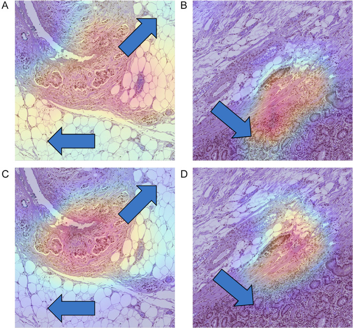
Grad‐CAM visualization of sample patch images. The Grad‐CAM provides insights into the areas of focus of the model. The upper row panels (A, B) depict the Grad‐CAM outputs of the weak models, while the lower row panels (C, D) illustrate the Grad‐CAM outputs of the strong models. Noteworthy, differences between the Grad‐CAM outputs of the weak and strong models are indicated by arrows. The focused area of the strong model appears comparatively compressed, effectively capturing the patterns indicative of LI‐positivity, in contrast to the wide and distributed focus areas observed in the weak models. Furthermore, panel (B) demonstrates the weak model's confusion between gland cell structures and LI‐positive patterns.

Discussion

In this study, we aimed to develop a model for detecting LI foci in gastric cancer using a deep neural network. Despite the importance of LI detection in gastric cancer, several studies have been conducted because of the difficulty of gathering annotated datasets [4, 6, 12, 13]. To mitigate this issue, we employed hard negative mining approaches that utilize weakly labeled datasets to train a robust classification model. With hard negative mining, the model classification performance improved considerably. Specifically, the strong model showed an improved classification performance of 2.88% for AUROC, 2.17% for AUPRC, 5.83% for the F1 score, 6.49% in sensitivity, and 4.72% in specificity. In subsequent ablation studies, the use of hard negative mining in the weakly labeled dataset improved the classification performance under both perturbing the entire dataset (limited dataset) and positive label‐only conditions (imbalanced dataset).

The LI classification model training process consisted of two stages: weak and strong model training, which are based on boosting algorithms, a widely adopted strategy in the field of machine learning. The LI region was identified by a distinct pattern consisting of a small tumor cluster surrounded by circular or elliptical spheres representing lymphatic vessels. However, the model was susceptible to confusion with hyperplastic crypts, which had a small tumor cluster surrounded by space and micropapillary patterns, as shown in Figure 6A,B. To mitigate this issue, we employed hard negative mining, a technique that queried highly confused patch images from weakly labeled negative datasets. We empirically selected the Euclidean distance to measure the similarity between false‐positive patch images and weakly labeled patch images.

Li et al achieved remarkable performance in classification tasks using hard negative mining, similar to our proposed approach [11]. However, there are two main differences between the proposed approach and that of Li et al: Li et al utilized a weakly labeled dataset and reweighed the sampling weight of the training data. In contrast, our approach queried hard samples from a weakly labeled dataset stored in a hospital's database. Consequently, the model was trained using various sample features. Li et al used K‐means clustering to identify similar samples in feature dimensions. In contrast, we applied a simple Euclidean (L2) distance to the feature dimensions. The K‐means clustering method requires hyperparameters, including the number of clusters (K), which must be set by the researcher. Further studies are required to identify the optimal K parameters. Therefore, in real‐world applications, querying N similar images is a more feasible approach.

Previous studies that detected LI utilized the DeepLabV3 architecture to predict LI foci with a semantic mask [12, 13]. This task of semantic segmentation is more complex than that of a classification model because it necessitates pixel‐level prediction and final classification output. Although semantic segmentation provides more detailed information about foci, such as the coarseness of the edge, size of the LI foci, and shape of the LI foci, it requires more sophisticated training procedures and pixel‐level annotated mask labels. However, in line with the diagnosis of LI, we hypothesized that the presence of LI is the most crucial factor rather than the size, shape, and form of the LI foci. Thus, we employed a straightforward classification approach for our model training procedures. Several studies proposed weakly supervised learning‐based methods for semantic segmentation. Despite this aspect, the task remains challenging and offers ample opportunity for further improvement [29, 30]. Furthermore, with Grad‐CAM visualization, we observed that the model focused on the LI foci rather than other areas, and the focused area was slightly wider than the semantic segmentation approaches demonstrated in previous studies. However, this limitation was offset using simple models and weakly labeled datasets.

The t‐SNE visualization results (Figure 5) obtained after hard negative mining show that false positives have a significantly larger feature distance from true positives. This indicates that the model was capable of effectively discerning the differences in features between false positives and true positives. The proposed method is noteworthy for its independence from the structure of the model and the features of the data, rendering it easily adaptable to models with varying structures or for the detection of different lesions. Consequently, it facilitates the robust classification of existing false and true positives, as evidenced by the t‐SNE results, and gains from data augmentation through the inclusion of weakly labeled datasets.

In general, the performance of machine learning models benefits from substantial training data; however, obtaining extensive healthcare data is challenging due to privacy concerns, collection costs, and other factors. Moreover, labeling such data is costly, often requiring specialized knowledge and expertise. To simulate a plausible situation of constructing a machine learning model applicable to a broad medical setting, we collected data from a single year, comprising 81 patients and 115 WSIs. Theoretically, both hard‐labeled datasets and weakly labeled datasets could be expanded to the entire set of electronic medical record data. However, this is not feasible due to the associated expenses in terms of labeling and computational resources. By incorporating hard negative samples within the weakly labeled dataset, we were able to develop a robust model while minimizing labeling costs.

In this study, we focused on a classification task for predicting the presence or absence of LI. Notably, one of the primary aims of LI detection is to predict lymph node metastasis, which is a critical factor in determining cancer prognosis. To establish the relationship between lymph node metastasis and LI, our future work will be extended to predicting lymph node metastasis based on LI prediction. In addition, we employed hard negative mining to assess similarity at the patch level. This approach has the potential to expand into the domain of image retrieval, contributing to the augmentation of weakly labeled datasets at both WSI and patch levels through image retrieval techniques. [31] In future work, our aim is to advance this methodology by integrating image retrieval and hard negative mining at the WSI level, aiming to alleviate labeling challenges and enhance model performance.

In conclusion, we aimed in this study to demonstrate the feasibility of utilizing a deep learning‐based approach to predict and detect LI in gastric cancer using high‐resolution digital pathology data. We employed a convolutional neural network and a hard negative mining strategy to reduce the number of false‐positive predictions. Our results demonstrate the potential of this approach to provide a valuable tool for pathologists and oncologists in managing gastric cancer patients, while also advancing deep learning algorithms for medical imaging applications (AUROC, 0.9738; AUPRC, 0.9501). Furthermore, this study highlights the efficacy of the hard negative mining approach in improving the performance of deep learning models, while reducing the time and cost associated with generating hard labels.

Author contributions statement

JL and JS contributed to the design of the research. HK and JS contributed to data acquisition. JL contributed to data analysis and modeling. JL, SA and JS wrote the manuscript. All authors have given their consent to the final version of the manuscript.

Data availability statement

The dataset for developing the model used in this study is freely available at the following link: https://zenodo.org/records/10020633. The source code for developing the model used in this study is freely available at the following link: https://github.com/jonghyunlee1993/LI_classification_with_hard_negative_mining.

References

- 1. Sung H, Ferlay J, Siegel RL, et al. Global cancer statistics 2020: GLOBOCAN estimates of incidence and mortality worldwide for 36 cancers in 185 countries. CA Cancer J Clin 2021; 71: 209–249. [DOI] [PubMed] [Google Scholar]
- 2. Lambert AW, Pattabiraman DR, Weinberg RA. Emerging biological principles of metastasis. Cell 2017; 168: 670–691. [DOI] [PMC free article] [PubMed] [Google Scholar]
- 3. Amin MB, Greene FL, Edge SB, et al. The eighth edition AJCC cancer staging manual: continuing to build a bridge from a population‐based to a more “personalized” approach to cancer staging. CA Cancer J Clin 2017; 67: 93–99. [DOI] [PubMed] [Google Scholar]
- 4. Fujikawa H, Koumori K, Watanabe H, et al. The clinical significance of lymphovascular invasion in gastric cancer. In Vivo 2020; 34: 1533–1539. [DOI] [PMC free article] [PubMed] [Google Scholar]
- 5. Kim H, Kim J‐H, Park JC, et al. Lymphovascular invasion is an important predictor of lymph node metastasis in endoscopically resected early gastric cancers. Oncol Rep 2011; 25: 1589–1595. [DOI] [PubMed] [Google Scholar]
- 6. Kim Y‐I, Kook M‐C, Choi JE, et al. Evaluation of submucosal or lymphovascular invasion detection rates in early gastric cancer based on pathology section interval. J Gastric Cancer 2020; 20: 165. [DOI] [PMC free article] [PubMed] [Google Scholar]
- 7. Kwee RM, Kwee TC. Predicting lymph node status in early gastric cancer. Gastric Cancer 2008; 11: 134–148. [DOI] [PubMed] [Google Scholar]
- 8. Jarkman S, Karlberg M, Pocevičiūtė M, et al. Generalization of deep learning in digital pathology: experience in breast cancer metastasis detection. Cancers (Basel) 2022; 14: 5424. [DOI] [PMC free article] [PubMed] [Google Scholar]
- 9. Srinidhi CL, Martel AL. Improving self‐supervised learning with hardness‐aware dynamic curriculum learning: an application to digital pathology. In Proceedings of the IEEE/CVF International Conference on Computer Vision , 2021; 562–571.
- 10. Pati P, Foncubierta‐Rodríguez A, Goksel O, et al. Reducing annotation effort in digital pathology: a co‐representation learning framework for classification tasks. Med Image Anal 2021; 67: 101859. [DOI] [PubMed] [Google Scholar]
- 11. Li M, Wu L, Wiliem A, et al. Deep instance‐level hard negative mining model for histopathology images. In Medical Image Computing and Computer Assisted Intervention – MICCAI 2019: 22nd International Conference, Shenzhen, China, October 13–17, 2019, Proceedings, Part I 22. Springer, 2019; 514–522.
- 12. Ghosh A, Sirinukunwattana K, Khalid Alham N, et al. The potential of artificial intelligence to detect lymphovascular invasion in testicular cancer. Cancers (Basel) 2021; 13: 1325. [DOI] [PMC free article] [PubMed] [Google Scholar]
- 13. Chen J, Yang Y, Luo B, et al. Further predictive value of lymphovascular invasion explored via supervised deep learning for lymph node metastases in breast cancer. Hum Pathol 2023; 131: 26–37. [DOI] [PubMed] [Google Scholar]
- 14. Ren S, He K, Girshick R, et al. Faster r‐cnn: towards real‐time object detection with region proposal networks. In NIPS'15: Proceedings of the 28th International Conference on Neural Information Processing Systems ‐ Volume 1, 2015; 91–99. https://dl.acm.org/doi/10.5555/2969239.2969250
- 15. Son JW, Hong JY, Kim Y, et al. How many private data are needed for deep learning in lung nodule detection on CT scans? A retrospective multicenter study. Cancers (Basel) 2022; 14: 3174. [DOI] [PMC free article] [PubMed] [Google Scholar]
- 16. Tang H, Kim DR, Xie X. Automated pulmonary nodule detection using 3D deep convolutional neural networks. In 2018 IEEE 15th International Symposium on Biomedical Imaging (ISBI 2018). IEEE, 2018; 523–526.
- 17. Qin Y, Zheng H, Zhu Y‐M, et al. Simultaneous accurate detection of pulmonary nodules and false positive reduction using 3D CNNs. In 2018 IEEE International Conference on Acoustics, Speech and Signal Processing (ICASSP). IEEE, 2018; 1005–1009.
- 18. Gong L, Jiang S, Yang Z, et al. Automated pulmonary nodule detection in CT images using 3D deep squeeze‐and‐excitation networks. Int J Comput Assist Radiol Surg 2019; 14: 1969–1979. [DOI] [PubMed] [Google Scholar]
- 19. Nagpal K, Foote D, Liu Y, et al. Development and validation of a deep learning algorithm for improving Gleason scoring of prostate cancer. NPJ Digit Med 2019; 2: 48. [DOI] [PMC free article] [PubMed] [Google Scholar]
- 20. Gutiérrez Y, Arevalo J, Martánez F. Multimodal contrastive supervised learning to classify clinical significance MRI regions on prostate cancer. In 2022 44th Annual International Conference of the IEEE Engineering in Medicine & Biology Society (EMBC). IEEE, 2022; 1682–1685. [DOI] [PubMed]
- 21. Xue C, Dou Q, Shi X, et al. Robust learning at noisy labeled medical images: applied to skin lesion classification. In 2019 IEEE 16th International Symposium on Biomedical Imaging (ISBI 2019). IEEE, 2019; 1280–1283.
- 22. Zhang X, Liang Y, Li W, et al. Development and evaluation of deep learning for screening dental caries from oral photographs. Oral Dis 2022; 28: 173–181. [DOI] [PubMed] [Google Scholar]
- 23. Bria A, Marrocco C, Tortorella F. Addressing class imbalance in deep learning for small lesion detection on medical images. Comput Biol Med 2020; 120: 103735. [DOI] [PubMed] [Google Scholar]
- 24. Nagtegaal ID, Odze RD, Klimstra D, et al. The 2019 WHO classification of tumours of the digestive system. Histopathology 2020; 76: 182–188. [DOI] [PMC free article] [PubMed] [Google Scholar]
- 25. Arigami T, Natsugoe S, Uenosono Y, et al. Lymphatic invasion using D2‐40 monoclonal antibody and its relationship to lymph node micrometastasis in pN0 gastric cancer. Br J Cancer 2005; 93: 688–693. [DOI] [PMC free article] [PubMed] [Google Scholar]
- 26. Yonemura Y, Endou Y, Tabachi K, et al. Evaluation of lymphatic invasion in primary gastric cancer by a new monoclonal antibody, D2‐40. Hum Pathol 2006; 37: 1193–1199. [DOI] [PubMed] [Google Scholar]
- 27. van der Maaten L, Hinton G. Visualizing data using t‐SNE. J Mach Learn Res 2008; 9: 2579–2605. [Google Scholar]
- 28. Selvaraju RR, Cogswell M, Das A, et al. Grad‐CAM: visual explanations from deep networks via gradient‐based localization. Int J Comput Vis 2020; 128: 336–359. [Google Scholar]
- 29. Chen Z, Tian Z, Zhu J, et al. C‐CAM: causal CAM for weakly supervised semantic segmentation on medical image. In 2022 IEEE/CVF Conference on Computer Vision and Pattern Recognition (CVPR). New Orleans, LA: IEEE, 2022; 11666–11675.
- 30. Zhou T, Zhang M, Zhao F, et al. Regional semantic contrast and aggregation for weakly supervised semantic segmentation. In 2022 IEEE/CVF Conference on Computer Vision and Pattern Recognition (CVPR) . New Orleans, LA: IEEE, 2022; 4299–4309.
- 31. Chen C, Lu MY, Williamson DFK, et al. Fast and scalable search of whole‐slide images via self‐supervised deep learning. Nat Biomed Eng 2022; 6: 1420–1434. [DOI] [PMC free article] [PubMed] [Google Scholar]
Associated Data
This section collects any data citations, data availability statements, or supplementary materials included in this article.