

Abstract
Anomaly detection (AD) aims to determine if an instance has properties different from those seen in normal cases. The success of this technique depends on how well a neural network learns from normal instances. We observe that the learning difficulty scales exponentially with the input resolution, making it infeasible to apply AD to high-resolution images. Resizing them to a lower resolution is a compromising solution and does not align with clinical practice where the diagnosis could depend on image details. In this work, we propose to train the network and perform inference at the patch level, through the sliding window algorithm. This simple operation allows the network to receive high-resolution images but introduces additional training difficulties, including inconsistent image structure and higher variance. We address these concerns by setting the network’s objective to learn augmentation-invariant features. We further study the augmentation function in the context of medical imaging. In particular, we observe that the resizing operation, a key augmentation in general computer vision literature, is detrimental to detection accuracy, and the inverting operation can be beneficial. We also propose a new module that encourages the network to learn from adjacent patches to boost detection performance. Extensive experiments are conducted on breast tomosynthesis and chest X-ray datasets and our method improves 8.03% and 5.66% AUC on image-level classification respectively over the current leading techniques. The experimental results demonstrate the effectiveness of our approach.
Keywords: Anomaly detection, data augmentation, medical image analysis, self-supervised learning
I. Introduction
Anomaly detection refers to the technique that only requires normal instances during training and determines an instance as abnormal if it contains properties that have not been seen before. This technique has drawn much attention in the community of medical image analysis [1]–[3] because of the natural rarity of diseases and the high cost of annotating the abnormalities. Furthermore, the process of identifying unexpected cases that differ from health references aligns with the behavior of human experts in clinical practice. The lack of labeled images also prevents the success of general supervised deep-learning-based approaches, which have been shown to perform well only with enough labeled training samples [4], [5].
Most existing anomaly detection works in the medical imaging f ield rely on solving a reconstruction task. During training, only healthy images are used, and thus the reconstruction error of the network is expected to be higher for abnormal inputs than for healthy ones. Two common network structures for solving the reconstruction task are auto-encoder (AE) [6] and generative adversarial network (GAN) [7]. AEs consist of an encoder that maps input images to a feature space and a decoder that maps the encoded features back to the image space. GANs include a generator that creates a fake image and a discriminator that determines if input images are real or fake. Both structures have undergone significant improvements [3], [8]–[10], and more advanced structures, such as diffusion model [11], are utilized to enhance the reconstruction quality, allowing for better distinguish between normal and abnormal inputs.
By convention, reconstruction-based methods for anomaly detection in medical images resize input images to a low resolution1, i.e., 256×256, to manage the training difficulty that exhibits quadratic growth with respect to the input size. However, the low resolution can be significantly smaller than that of the original images acquired from common modalities, e.g., breast tomography and x-ray. While adding more upsampling layers can enhance the resolution of networks’ output, such an operation can also lead to training instability and nonsensical outputs [12]. In this work, we propose a simple approach that leverages the sliding window (SW) algorithm to enable the network to process high-resolution images. As shown in Fig. 1, the SW algorithm allows the same framework to handle higher-resolution images by feeding patches instead of images to a neural network. During inference, we iterate over a full image through the SW algorithm, resulting in patches.
Fig. 1.
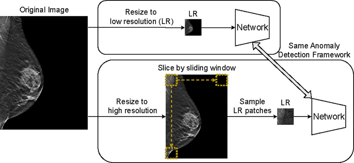
Top block: standard pipeline where images are resized to low resolution and fed to networks. Bottom block: new pipeline with the sliding window algorithm. Images are resized to high resolution and image patches are fed to networks. The overall resolution of input images is increased without modifying the structure of the network.
Although SW alleviates the over-downsampling issue, receiving patches instead of images increases the complexity of the reconstruction task greatly since image patches are more diverse and not aligned. To overcome this challenge, we propose a new framework for anomaly detection through self-supervised learning (SSL), as shown in Fig. 2. One of the most common and effective objectives of SSL is to learn features that are invariant against data augmentations. To achieve this objective, we use the Barlow Twins loss [13] that maximizes the similarity between features of two distorted views of the same images along the batch dimension. Specifically, given two representations with showing the batch size and the hidden dimension, BT defines the similarity matrix as while traditional SSL works deploy . During inference, we first obtain a memory bank of all training features where stands for training sample sizes. To align with the optimization dimension, we treat a testing feature representation as neurons activated at locations, and propose the anomaly score of each neuron as the difference between its activation on the testing image and the most similar training image. The maximum neuron-level anomaly score is used as the image-level anomaly score. The proposed method is named Sliding-Window based Self-Supervised Learning (SWSSL) to highlight the usage of the sliding window algorithm and self-supervised learning for anomaly detection.
Fig. 2.

Overview of the proposed anomaly detection approach. Left: Input image after resizing to high resolution. Each dot presents the center of a non-zero image patch selected by the sliding window algorithm. Training phase: An image patch (blue box) and its neighbor patch (red box) are selected for the Barlow Twins loss and Continuity Preserving loss, the details of both loss are shown in Fig. 3. Both the output from the encoder and projector is in , where is the hidden size. Testing Phase: All training patches are passed through the encoder and stored in a memory bank. The anomaly score is defined as the minimum distance between the feature of a testing neuron and all training neurons.
The choice of augmentations used for SSL is crucial for learning useful representations [14]. In this study, we focus on augmentations suitable for medical images. In particular, we find the cropping then resizing operation, which creates adjacent patches as inputs and is a key augmentation function in natural imaging augmentations [15], [16], is not suitable for the target medical images. The resizing operation creates unnecessary augmentations when training and testing images are acquired with the same protocol and can unreasonably modify pixel densities, a property that can indicate the presence of diseases. For example, a zoom-in optical nerve can lead to the mis-classification of papilledema. Therefore, we remove this operation and propose Continuity Preserving (CP) loss, which encourages the network to encode spatially close patches similarly, as a substitute. CP achieves the same functionality of cropping then resizing by learning from adjacent patches. Another useful augmentation we discover is the inverting operation, which allows the network to only focus on meaningful structures in medical images such as bones in chest images and lesions in breast tomosynthesis.
To evaluate the effectiveness of our proposed SWSSL, we conduct experiments on two datasets with different organs and modalities: Breast Tomosynthesis [17] and Chest X-ray [18]. To demonstrate the generalizability of our approach, we compare to a wide range of anomaly detection methods that receive 256×256 images as inputs, as well as their SW-aided upsampling versions that receive 1024×768 for breast and 1024×1024 for chest images. Our method achieves state-of-the-art performance on both datasets, with an AUC of 0.7848 for breast and 0.8877 for chest, surpassing the runner-up methods by 8.03% and 5.66% AUC, respectively. These results demonstrate that SWSSL is a powerful and effective method for anomaly detection in medical images, and that it outperforms existing methods by a significant margin.
The main contributions of this paper are summarized as follows.
We alleviate the problem of over-downsampled images in anomaly detection by proposing SWSSL, a novel self-supervised learning-based framework for anomaly detection.
We observe that when learning augmentation-invariant representations of medical images, the inverting operation can be beneficial while the cropping then resizing operation is detrimental.
The Continuity Preserving loss is proposed to accommodate the removal of cropping then resizing by encouraging the representations of adjacent patches similar.
Experimental results demonstrate the effectiveness of our method on different organs collected by different modalities.
II. Related Works
A. Anomaly detection
Anomaly detection aims to determine if an instance has properties different from those seen in normal instances. This technique has been applied to various problems, including manufacturing defect detection [19]–[21], video surveillance [22]–[24], and medical image analysis [1]–[3]. Several algorithms have been proposed to address this problem. For example, one-class classifier, either parameterized by deep neural networks [25], [26] or SVMs [27], minimizes the volume of a hyper-sphere that encloses the representations of normal data, and detects anomalies as samples falling outside. Gaussian mixture models learn the distribution of normal data and detect anomalies as samples with low probabilities [28]–[30]. Transfer-learning-based methods have also been proposed, such as the student-teacher framework where the teacher network distills knowledge from pre-trained networks on ImageNet [31]. Recent work [32] shows that directly using middle-level features from a pre-trained network achieves near-perfect discrimination between normal data and anomalies.
Reconstruction-based methods are another popular set of approaches for anomaly detection, where the methods aim to reconstruct the input data and use pixel-wise differences to identify anomalies. Auto-encoders (AE) are widely used to learn the reconstruction function [33]–[36], and their objective function can be improved to further boost the detection performance [8], [37]. Alternatively, generative adversarial network (GAN) based methods have also been proposed. AnoGAN [1] uses GAN to reconstruct the inputs and proposes an iterative process to determine the latent code for a query image, while f-AnoGAN [9] replaces the iterative search process with a trainable encoder to accelerate the search process. ALAD [38] proposes a bi-directional GAN to increase inference efficiency as well as improve training stability. Other methods estimate the probability distribution of normal training data and consider data with low probabilities as anomalies [39], [40]. The network structures have also been extended beyond autoencoders and GANs to obtain a normal reconstruction of some input test image, but these literatures follow the same concept of detecting anomalies via discrepancies between the input image and its normal reconstruction [11], [41]. Finally, Pinaya et al. [42] uses denoising diffusion models in the normal image feature space to translate anomalies at the feature-level to pixel-level anomaly segmentation. Although these reconstruction-based methods have achieved leading performance in medical imaging anomaly detection, their input sizes are often limited to low resolutions, i.e., 256×256. Higher resolution inputs can lead to unsatisfactory reconstruction fidelity. On the other side, our proposed method can process high-resolution images by slicing patches during training.
B. Self-supervised learning
The goal of self-supervised learning (SSL) is to learn effective visual representations without the need for human supervision. In the context of AD, SSL can be achieved by solving proxy tasks. For example, some works [43]–[45] apply rotation and translation to the images and aim to predict the applied augmentation. Li et al. [46] extends this method by introducing a new type of augmentation that cuts and pastes an image patch at a random location, which is further improved to make the pasting process seamless [47]. Tian et al. [48] trains an image representation encoder with a proxy task that classifies whether normal images have strong or weak augmentations. However, in medical imaging, proxy tasks that assume anomalies as augmented versions of original images may not be accurate, as an anomaly image could represent the presence of tumor regions, which cannot be artificially generated from normal images.
An alternative branch of SSL is to find representations that are robust against distortions. Contrastive learning-based methods [14], [49], [50] achieve this goal by first applying different augmentation operations to a batch of images and calculating a similarity matrix between the two augmented groups. Then the objective is to increase the similarity score for different augmentations of the same image and decrease the score for different image pairs. Other methods [51]–[53] introduce the distortion by creating asymmetrical network architecture, i.e., adding stop-gradient on one of the branch and introducing the predictor network. However, these works either require significantly large batch size to learn useful representations or particular implementation choices to avoid non-trivial learning dynamics, hindering the application to anomaly detection. Barlow Twins (BT) [13] adopts a similar approach of calculating a similarity matrix between two groups of augmented images and differs with other works in that the similarity is computed among the batch dimension. The novel loss function prevents a trivial solution and obtains a good performance with moderate batch size. Thus, we select BT as the learning objective.
III. Method
This work aims to develop a novel framework for anomaly detection using only normal images. Unlike most existing approaches that use low-resolution images, typically 256×256, our framework is designed to handle high-resolution images, i.e., 1024 × 1024. In this section, we introduce the proposed anomaly detection method in detail.
A. Pipeline
The proposed SWSSL model is composed of a feature extraction network followed by a projector network . Both networks are deep learning-based with trainable parameters and respectively. The training and testing process are presented in Fig. 2, with the details of some components shown in Fig. 3. During training, we first crop an image patch from the full image . Two distorted views of the image patch are fed through and sequentially and the outputs are optimized using the Barlow Twins loss, which aims to minimize the difference of the two representations along the batch dimension. The Continuity Preserving loss is further proposed to minimize the difference between the representation of adjacent image patches. This objective is implemented by matching the cosine similarity between two representations with their overlapped area.
Fig. 3.

Details of the Barlow Twins loss (green box) and continuity preserving loss (red box). refers to cosine similarity.
The inference process of the proposed SWSSL model involves using the sliding window algorithm to slice over all training images. Each resulting image patch is then encoded by and stored in a memory bank. The projector is not utilized during inference. Similarly, a testing image is processed with the same procedure. We propose a novel strategy to compute the difference between the representation of testing and training images at the neuron level. Specifically, the behavior of a neuron on an image is defined as the cumulative activation of the neuron across all patches generated from that image. Then we can calculate the neuron-level anomaly score as the difference of the behavior of a neuron on the test image and the most similar training image. Since an image is defined as an abnormal image if some regions of it contain abnormal cases, we use the maximum neuron anomaly score as the image anomaly score.
B. Upsampling through sliding window algorithm
Learning a holistic representation of high-resolution images is hardly feasible for modern neural networks. To alleviate this problem, we propose to crop image patches as inputs to the network. In this way, the network can understand the full image by accumulating knowledge from local representations at different locations. In particular, we use the sliding window (SW) algorithm to slide over an input image during inference. Formally, for a full image , a sliding window algorithm with patch size and stride size divides the full images into a set of image patches . Given patch indexes we have
| (1) |
The patch indexes are bounded by and respectively. Although simple, this strategy differs from works that receive local information by using features from shallow layers in the network [32], [54], [55]. These methods are not obtaining true local-level information from the perspective of the receptive field. For example, the receptive field of the 2nd layer of Resnet50 is 99 and the 3rd layer is 291, which is larger than the size of most input images [56]. An image patch is fed to the network . We also remove the zero patches, i.e., all pixels in this patch are black, in as they are not informative. Empirically, we find the algorithm exhibits very similar performance when inputs are sampled from the pre-defined set or randomly.
C. Self-supervised Learning Module
The goal of our network, , is to learn effective visual representations without human supervision. This is achieved by learning representations that are invariant under different distortions, and we employ Barlow Twins (BT) [13] as the objective. Specifically, for a batch of image patches with size and two pre-defined data augmentation operations and , we can obtain two distorted views of the input image and . The two distorted batches are fed to and sequentially to obtain two batches of embeddings , which are then normalized along the batch dimension. That is, each column of the representation is normalized to 0 mean and standard deviation. Using an additional projector network to encode the images follows the convention of self-supervised learning and has been empirically demonstrated to enhance the learning process [14]. The projector is discarded during inference. The BT’s loss function can be defined as
| (2) |
where controls the weight for non-diagonal elements, and is the cross-correlation matrix computed between the outputs of the two identical networks along the batch dimension:
| (3) |
where indexes batch samples and index the vector dimension of the network’s outputs.
D. Choices of augmentation functions
The selection of augmentation operations plays an important role in defining the task of learning augmentation-invariant representations. Our initial choice of the augmentation operations follows that of the BT [13]. A recent work [14] discusses two types of data augmentation that are important for the network to learn effective representations. The first type of augmentation involves appearance transformation, such as image distortion (including color dropping, brightness, contrast, saturation, and hue), Gaussian blur, and Sober filtering. Since our target datasets are medical images that are generally grayscaled, we exclude the distortions along the color channel. Furthermore, we find that the structure of each input image is not altered during appearance transformation. Recall that the objective of BT is to learn distortion-invariant features, suggesting that the network prioritizes learning this structure information. Thus, we propose to include the inverting operation as a straightforward way to enhance structure awareness of the network. Such an idea aligns with an earlier work [57] if we consider inverting as an extreme case of style transfer. Fig. 4 visualizes the appearance transformation augmentation used in this work.
Fig. 4.
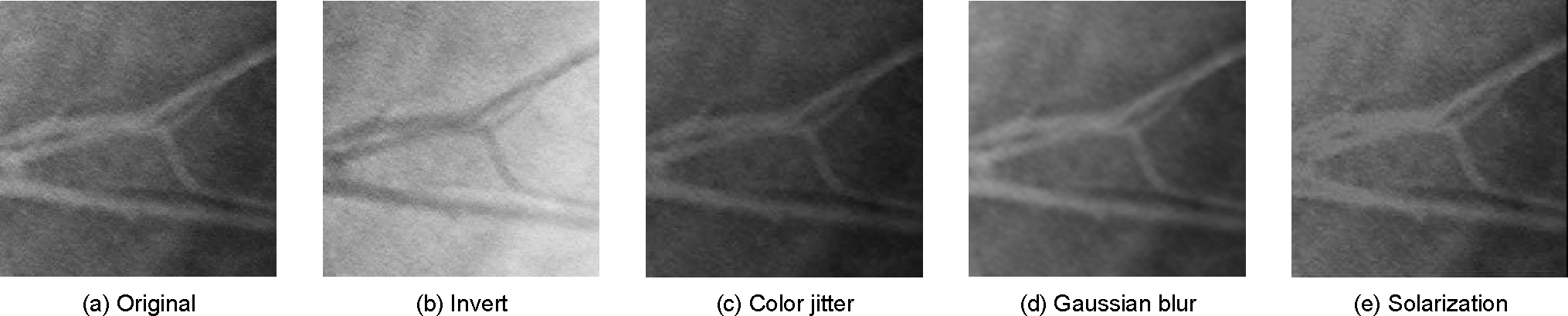
Augmentation operations used in this framework. All operations are applied stochastically to both distorted images except inverting, which is only applied to one of the images.
The other type of augmentation discussed in [14] involves spatial/geometric transformation of data, such as cropping, resizing, rotation, and cutout. In particular, the cropping then resizing operation has been found to be a key component for effective representation learning by providing overlapping and global to local image pairs [15]. Both types of image pairs are shown in Fig. 5. However, we argue that the resizing operation is not applicable to medical images that are taken under the same protocol, i.e., the camera viewpoint is consistent over different images. The resizing operation could break this property and introduce unnecessary difficulty to the training process. Moreover, the size of some organs/tissues can be an indication of certain diseases. Therefore, we propose to remove the cropping then resizing operation. However, without this operation, the network cannot learn from the overlapping and global-to-local image pairs. While it is not feasible to create global-to-local pairs without resizing, we propose a novel objective that generates and learns from overlapping pairs. Specifically, the objective encourages the representations of overlapping pairs to be similar. As intuitively, this objective encourages the network to be a continuous function, we name the objective as the Continuity Preserving (CP) loss. We show the details of CP’s objective next.
Fig. 5.

Two types of image pairs effective for self-supervised learning generated by the cropping then resizing operation. The proposed Continuity Preserving loss enables the generation of overlapping pairs while global-to-local pairs are infeasible to generate without resizing.
E. Continuity Preserving loss
To generate overlapped image pairs, we first define the neighborhood of an image patch as
| (4) |
where returns the patch indexes defined in Eq. (1). Then, for each input image patch , we sample its adjacent patch and similarly, get its representation . When receiving two overlapped patches, traditional SSL approaches [14] treat them as different distortions of the same image and encourage their representation to be the same. However, this can be a strict objective as the ideal solution is to ignore the non-overlapping regions in each patch that may contain useful information. We thus propose an approximate objective in our Continuity Preserving loss by making representations from adjacent patches similar. Following BT, we can define similarity as the correlation between and . That is, we want to minimize
where is the cross-correlation matrix computed between two normalized representations and . Then, we can set the target similarity, , i.e., 0.5, to reflect that the two terms are positively correlated with each other. This objective, however, does not improve anomaly detection performance in practice. One explanation is that applying an additional constraint on the same dimension can lead to contradictory objectives. Thus, we consider applying the objective on the other dimension, i.e., at the instance level. Formally, given the unnormalized representation and , the Continuity Preserving loss is computed as
| (5) |
where computes the cosine similarity between the representations of an image patch and its neighbor as:
| (6) |
is a target function that gives the approximate similarity score based on the actual overlapped area of the two patches. Specifically, denote the patch index of and as and respectively, we have
| (7) |
We further restrict the fraction to be 0 when . Recall that the motivation of this objective is to encourage the encoding network to be continuous. To elaborate on this intuition, let us consider the target network , which encodes image patches into the feature space: . By having the regularization term (Eq. 5), has the constraint where a minor change in the image space only leads to a proportional change in the feature space. Moreover, if we restrict the input space to the set of patches sampled from the same image, we can define the metric on the image space as , where comes from Eq. 4. The metric on the feature space can be defined as , where is defined in Eq. 6. Then the function can exhibit Lipschitz continuity if the regularization is satisfied.
Furthermore, we can extend the regularization to different augmentations of the same patch and with the goal of a perfect match, i.e.,
| (8) |
which has an optimal solution when . Their target similarity is set to 1 because there is no spatial difference between the two inputs, i.e., . Note that the optimal solution of this term aligns with the first term of Barlow Twin’s loss. As the two objectives share the same optimal solution, adding this constraint can improve the performance of the network. The overall objective for the network includes Eq. 2, Eq. 5, and Eq. 8:
| (9) |
where controls the contribution of the Continuity Preserving loss.
F. Evaluation
During the evaluation phase, we densely extract feature representations at the patch level through the sliding window algorithm (SW), for both training and evaluation data. This means a single image is presented by patch features and thus in , where is the set of patches obtained from SW and is the hidden dimension. All training samples are stored in a memory bank , where is the number of normal samples for training. Since the Barlow Twin loss regularizes the behavior of each component in the batch dimension, we propose a novel evaluation strategy to align with its principle. The pseudo-code to compute the anomaly score is shown in Alg. 1. Specifically, an encoded embedding in can be viewed as the behavior of different neurons, and thus the image feature in can be treated as each neuron activating times. Although the specific information acquired by each neuron cannot be tracked, we assume that the behavior of neurons will be more similar when inputs do not contain abnormalities than those do. To implement this idea, we define the anomaly score of each neuron as the difference between its activation on the testing image and the most similar training image. In this way, we can obtain a score map of all neurons in . The maximum score from the score map is used to detect anomalies at the image level.
Algorithm 1.
Pseudo-code for evaluation
|
Input: Test Image ; The Sliding Window Algorithm , returning image patches in ; Pretrained Network ; Training Memory Bank . Slice the testing image through the sliding window algorithm Initialize a tracking variable for image representation for each patch in with location do store the patch representation end for Initialize a tracking variable for d=1,2,...,D do Initialize a tracking variable for i=1,2,...,N do The L2 distance between a testing neuron and a training neuron at the same location end for The smallest distance indicates the level of abnormality for a neuron end for Return The most dissimilar neuron indicates the image level abnormality |
IV. Experiments
In this section, we validate the performance of the proposed SWSSL method in detecting anomalies from two modalities, i.e., lesions in breast tomosynthesis and pneumonia in chest X-ray. First, the experimental setup details are described, followed by the results comparing with state-of-the-arts on different datasets. Finally, we perform an ablation study to verify each proposed contribution.
A. Dataset
We select two publicly available datasets with different organs and collected by different modalities to evaluate the proposed approach.
1). DBT:
The breast cancer screening - digital breast tomosynthesis (BCS-DBT) [17] dataset contains data for 5,060 patients, split into normal, actionable, benign, and cancer groups. For training, we sample 6,245 healthy slices of DBT volumes from the training set, each of which comes from a different anatomical view and/or patient. We select 75 slices from the benign and cancer groups where each contains at least one radiologist-annotated tumor as the abnormal testing images and randomly sample the same number of slices from the normal group (without overlapping) as the normal testing images.
2). Chest X-ray:
The Chest X-ray dataset [18] consists of normal and pneumonia images collected from 6,480 patients. There are image-level annotations for each subject. The training dataset contains 1,349 normal images and the test set contains 234 normal images and 390 pneumonia images.
B. Experimental details
1). Implementation Details:
The optimizer is SGD and the learning rate is 5 × 10⁻⁶ for DBT and 10−4 for Chest X-ray. The images are resized to 1024 × 1024 and normalized to [−1, 1] for chest X-ray and 1024 × 768 and normalized by the mean and standard deviation from ImageNet [58] for breast tomosynthesis. The non-squared input size keeps the width/height ratio between original and resized breast tomosynthesis similarly. The selection of learning rate and normalization value follows the previous work [59]. Wide-Resnet 50 [60] (without final classification layer, 2048 output units) is used as the feature extraction network, and three linear layers, each with 2048 output units and batch normalization and rectified linear units used for non-linearity form the projection network. Patch size is set to 128 and stride size is 32 for both datasets. , following the original paper [13] and . The threshold to select neighbors is set to 3. Methods are trained for 50 and 20 epochs for DBT and Chest X-ray with mini-batch size 300. The final model is used for evaluation. All models are trained on a single NVIDIA RTX A6000. During the evaluation, the memory bank that tracks all training features is stored in RAM and the computation time between a testing image and the memory bank is 2.71 seconds for the DBT dataset and 0.62 seconds for the Chest X-ray dataset. The code is shared publicly2.
Image augmentations.
Following the discussion in Section III-C, consists of the following three augmentations with probabilities 0.8,1.0,0.0 on DBT and 0.8,0.1,0.2 on Chest X-ray:
Color jittering: the brightness and contrast of the image are shifted by a uniformly random factor over [0.6,1.4].
Gaussian blurring: applying a sequence of extended box filters with standard deviation uniformly sampled over [0.1, 2.0].
Solarization: inverting all pixel values above a threshold. We use the default threshold value of 128.
contains an additional invert operation at the beginning with probability 1.
2). Evaluation Metrics:
We calculate the Area Under Receiver Operation characteristic (AUC), F1-score, average classification accuracy (ACC), sensitivity (SEN), and specificity (SPE). F1-score is defined as the harmonic mean of precision and recall. The threshold used for evaluation is determined based on the best value of the F1-score for each dataset.
3). Baseline Methods:
We compare our method with several state-of-the-art anomaly detection methods, including Auto-Encoder (AE), Uncertainty AE3 [8], and SSIM-based AE4 [61] based anomaly detection method, f-Anogan5 [9], GANomaly6 [10], PatchCore 7 [32], PaDiM8 [54], Intra9 [62] and SALAD10 [59]. Some results on the Chest X-ray dataset are obtained directly from the previous work [59] and the rest are from our re-implementation. For each competing method, we obtain the original code whenever publicly available and apply the recommended hyperparameters. The models are re-trained on our dataset with the same preprocessing procedure, except for resizing. For PaDiM and PatchCore, we use the same backbone, Wide-Resnet 50, for embedding extraction. Since all methods but Intra are not specifically designed for high-resolution inputs, images are resized to 256 × 256. However, this may introduce a potential discrepancy in the comparison as our proposed method takes advantage of receiving high-resolution inputs. To address this concern, we also apply the sliding window (SW) algorithm (denoted as “+SW”) to all competing methods, except PaDiM, and PatchCore. We excluded these two methods since they require storing image features from the middle layer of all training samples, which exceeds our hardware capacity. The training procedure for the competing methods is similar to ours, where an image patch is fed to the network. During inference, we iterate over the input images using the sliding window and obtain the reconstruction error for each patch. The largest error among the patches is used as the image-level anomaly score. Intra employs a similar patch-based strategy to partition the images into square regions of fixed size and thus we feed it with high-resolution inputs directly.
C. Detection Performance on DBT
We first evaluate the performance of our SWSSL and state-of-the-art approaches on the DBT dataset. The experimental results are presented in Table I. Based on the size of inputs, we split the methods by their larger input resolution, i.e., 256 and 1024. It can be observed that our method outperforms all methods with low-resolution inputs. PatchCore and PaDiM exhibit moderate performance since they rely on the knowledge from the networks pre-trained on natural images. However, we observe no benefit of using more advanced reconstruction objectives and network structures than the baseline AE. This can be caused by the data property of DBT. Specifically, a breast usually does not occupy the full image. A simple per-pixel reconstruction loss does not consider the correlation among pixels, while other methods do and thus incorrectly treat these black regions as part of the captured breast. This increases the difficulty of the reconstruction task as the sizes of breasts vary.
TABLE I.
Performance results (AUC, F1(%), ACC(%), SEN(%), and SPE(%)) of different methods on DBT and Chest X-ray.
| DBT | Chest X-ray | Size | |||||||||
|---|---|---|---|---|---|---|---|---|---|---|---|
|
| |||||||||||
| AUC | F1 | ACC | SEN | SPE | AUC | F1 | ACC | SEN | SPE | ||
|
| |||||||||||
| AE | 0.7045 | 71.29 | 61.33 | 96.00 | 26.67 | 0.5987 | 77.20 | 63.40 | 98.97 | 3.86 | |
| UAE [8] | 0.6352 | 68.97 | 58.00 | 93.33 | 22.67 | 0.6806 | 78.18 | 66.19 | 96.68 | 15.02 | |
| SSIM-based AE | 0.6679 | 70.79 | 65.33 | 84.00 | 46.67 | 0.7937 | 81.16 | 72.87 | 93.33 | 38.62 | 256 |
| f-AnoGAN [9] | 0.4032 | 66.07 | 49.33 | 98.67 | 0.00 | 0.7546 | 81.00 | 74.00 | 88.97 | 36.48 | |
| GAnomaly [10] | 0.5125 | 67.30 | 54.00 | 94.67 | 13.33 | 0.7800 | 78.97 | 69.98 | 90.00 | 48.93 | |
| PaDiM [54] | 0.6585 | 60.05 | 63.33 | 92.00 | 34.67 | 0.7356 | 72.50 | 75.00 | 94.87 | 41.88 | |
| Patchcore [32] | 0.6484 | 64.54 | 64.67 | 70.67 | 58.67 | 0.8241 | 70.75 | 74.36 | 97.69 | 35.47 | |
| SALAD [59] | - | - | - | - | - | 0.8265 | 82.14 | 75.92 | 88.46 | 54.94 | |
|
| |||||||||||
| AE + SW | 0.6628 | 73.02 | 66.00 | 92.00 | 40.00 | 0.4521 | 76.80 | 62.34 | 99.74 | 0.00 | |
| UAE + SW | 0.4953 | 52.67 | 52.67 | 96.00 | 0.09 | 0.3576 | 76.80 | 62.34 | 99.74 | 0.00 | |
| SSIM-base AE + SW | 0.6027 | 68.18 | 53.33 | 100.00 | 0.07 | 0.7665 | 79.55 | 70.67 | 91.28 | 36.32 | |
| f-AnoGAN + SW | 0.5912 | 50.67 | 58.68 | 42.67 | 74.67 | 0.5009 | 77.00 | 62.66 | 100.00 | 0.01 | 1024 |
| GAnomaly + SW | 0.4638 | 57.14 | 48.00 | 69.33 | 26.67 | 0.4306 | 76.80 | 62.34 | 99.74 | 0.00 | |
| Intra [62] | 0.6233 | 69.52 | 57.33 | 97.33 | 17.33 | 0.6401 | 77.78 | 67.31 | 91.54 | 26.92 | |
| SWSSL (Ours) | 0.7848 | 77.91 | 74.67 | 89.33 | 60.00 | 0.8831 | 85.85 | 81.41 | 90.26 | 66.67 | |
When applying the sliding window algorithm to the competing methods, we observe little benefit from this operation. In particular, only the performance of AE is improved in terms of F1 score and accuracy at the cost of AUC, and all other methods result in a trivial output (the close to full sensitivity and zero specificity indicates that the network works best when predicting all inputs as abnormal). Such experimental results suggest that the reconstruction-based methods may not benefit from the sliding window algorithm because the input patches are not aligned and their variance is much higher than that of full images. The inpainting-based method, Intra [62], can make non-trivial predictions, but our network outperforms it by a large margin (16.15% AUC).
Furthermore, apart from AUC, our method achieves the best F1-score and ACC (77.91% and 74.67%) among all competing methods, outperforming the runner-up method (AE+SW) by 4.89% and 8.67% respectively. Although the sensitivity of SWSSL is less than most methods, our method achieves a much higher specificity, meaning it is more likely to reject healthy patients without lesions. Note that this is a particularly challenging task for DBT as lobules appear in both normal and lesion images. Some visual examples are shown in Fig. 6 to illustrate the difficulty of detecting anomalies for DBT scans. In some situations when sensitivity is of high interest, we can adjust the threshold selection strategy to prioritize sensitivity instead of the F1 score. In this case, our method achieves 100.00% sensitivity with 26.67% specificity.
Fig. 6.

Visual examples of normal and abnormal images from DBT where red boxes indicate lesion locations. These examples illustrate that lobules appear in both types of images and lesions can be either inside or outside the lobules.
D. Detection Performance on Chest
We further test our approach on the chest X-ray dataset. The experimental results are shown in Table I. Our method still outperforms all methods with both low and high-resolution inputs. Similarly, incorporating the SW algorithm does not improve the performance of reconstruction-based methods. The more severe performance degradation can be caused by the higher variance within chests, which contain multiple anatomical structures such as lungs and bones. However, note that when the original network performs well, i.e., SSIM-based AE (and AE in DBT), applying SW only decreases the performance slightly. Such an observation suggests that the SW algorithm may be beneficial to the network when its performance on low-resolution images is further improved. Compared with the results on the DBT dataset, the anomaly detection accuracy of all methods consistently increases. The underlying reason for the performance improvement is that pneumonia in chests is more apparent than the lesions in breasts, which vary greatly in size and location and can be visually similar to healthy tissues. Similarly in the situations when sensitivity is of high interest, by adjusting the threshold our method achieves 98.29% sensitivity with 34.62% specificity.
E. Ablation Study
We conduct a thorough ablation study to evaluate the effectiveness of the proposed method.
1). Augmentations for Barlow Twins:
One of the contributions of this paper is the selection of augmentation operations for the self-supervised learning module. To study the effectiveness of each operation change, we run a series of studies from the original augmentation operations to our final version. The evaluation phase is not changed during the study in this section. Since this is the major argument in this paper, we conduct the study on both datasets. Results on the DBT dataset are shown in Table II and on the Chest X-ray Dataset are shown in Table III.
TABLE II.
Performance Results (AUC, F1(%), ACC(%), SEN(%), and SPE(%)) of ablation studies on augmentation operations on DBT.
| BT | SW | Inv. | CP | AUC | F1 | ACC | SEN | SPE |
|---|---|---|---|---|---|---|---|---|
|
| ||||||||
| ✓ | 0.7291 | 72.28 | 62.67 | 97.33 | 28.00 | |||
| ✓ | ✓ | 0.7538 | 74.74 | 68.00 | 94.67 | 41.33 | ||
| ✓ | ✓ | ✓ | 0.7710 | 75.28 | 70.67 | 89.33 | 52.00 | |
| ✓ | ✓ | ✓ | ✓ | 0.7848 | 77.91 | 74.67 | 89.33 | 60.00 |
TABLE III.
Performance results (AUC, F1(%), ACC(%), SEN(%), and SPE(%)) of ablation studies on augmentation operations on Chest X-ray.
| BT | SW | Inv. | CP | AUC | F1 | ACC | SEN | SPE |
|---|---|---|---|---|---|---|---|---|
|
| ||||||||
| ✓ | 0.8005 | 73.97 | 77.88 | 93.33 | 52.14 | |||
| ✓ | ✓ | 0.8102 | 75.43 | 77.40 | 84.62 | 65.38 | ||
| ✓ | ✓ | ✓ | 0.8456 | 75.93 | 78.21 | 87.18 | 63.25 | |
| ✓ | ✓ | ✓ | ✓ | 0.8831 | 85.85 | 81.41 | 90.26 | 66.67 |
Barlow Twins (BT) means to train the network with unmodified augmentations. In particular, the cropping then resizing operation is used to obtain the input patches. This setting serves as the base model for the following comparisons. Note that despite no modifications being made to the Barlow Twins, this setting already outperforms all competing methods on the DBT dataset and gains similar performance as the SOTA performance on the Chest X-ray Dataset. This suggests that the overall framework, i.e., training with image patches and encoding full images in a raster-scan manner during testing, is an effective way for anomaly detection with high-resolution images.
Sliding Window (SW) highlights that the input images are sampled from the patch set generated by the sliding window algorithm rather than using the cropping then resizing operation. In this way, the resizing operation is excluded. This results in improvements in AUC for both datasets, demonstrating the ineffectiveness of changing the pixel densities through resizing when images are acquired through the same pipeline.
Inverting (Inv.) is an operation we find to be useful in learning representations robust to augmentations. In particular, we apply the inverting operation to one of the distorted images. This results in 1.72% improvements in AUC for the DBT dataset and 3.54% improvements for the Chest X-ray dataset. By encoding the representations of an image and its inverted version, we suppress the network from making inferences through the intensity of pixels. On the other hand, the transition of pixel intensity is preserved, which turned out to emphasize the physical texture of tissues in each image. This augmentation trick has been shown empirically beneficial in improving the model’s performance.
Continuity Preserving loss (CP) is the substitute loss we propose to alleviate the problem of missing adjacent patch information from removing the cropping then resizing operation. Adding this constraint improves the performance of the algorithm on both datasets, with significant improvements on the Chest X-ray datasets (3.75% AUC). The effectiveness of this component can be explained as that by encoding the adjacent patch similarly, the network implicitly obtains the global level information. This information is important to identify the abnormalities. For example in DBT scans, lesions caused by breast cancer can be visually similar to normal lobules but appear in some unusual locations. Determining these lesions requires the knowledge of the full tomosynthesis scans.
2). Continuity Preserving objective:
In this study, we consider a few variations in designing the Continuity Preserving loss. Results on the DBT dataset are shown in Table IV.
TABLE IV.
Performance results (AUC, F1(%), ACC(%), SEN(%), and SPE(%)) of ablation studies on Continuity Preserving loss on DBT.
| AUC | F1 | ACC | SEN | SPE | |
|---|---|---|---|---|---|
|
| |||||
| Batch Dim. | 0.7578 | 76.67 | 72.00 | 92.00 | 52.00 |
| Neigh. Only | 0.7833 | 76.65 | 74.00 | 85.33 | 62.67 |
| Same Only | 0.7545 | 73.47 | 65.33 | 96.00 | 34.67 |
| Full | 0.7848 | 77.91 | 74.67 | 89.33 | 60.00 |
Batch Dimension refers to the initial objective of the Continuity Preserving loss that increases the similarity along the batch dimension, i.e., Eq. III-E. It follows the regularization with Barlow Twins. However, this objective decreases the performance by 2.7% AUC. One explanation is that the target correlation is selected arbitrarily, i.e., 0.5, and all adjacent patches, despite their overlapping sizes, are treated equally.
Neighbor only means only the regularization on the adjacent patches is applied, i.e., Eq. 5. As the neighbor information encourages the network to learn inputs’ global information, exclusively applying this objective results in higher specificity (+2.67%) at the cost of AUC (−1.50%). Based on our primary selection metric (AUC), we select to include the other objective of Continuity Preserving loss.
Same only means only the regularization on the same image patch is applied, i.e., Eq. 8. This contradicts the objective of Continuity Preserving loss to learn the similarity between the representations of adjacent patches. Therefore, we observe a 3.03% AUC decrease.
3). Evaluation metric:
Recall that we treat the densely encoded image representation neurons activating at locations and thus compute the anomaly score as the difference between the activation of a neuron on the testing image and the most similar training image, i.e., .. In this section, we consider a more common way of treating as the representation of patches, each encoded into an embedding of length and evaluating the anomaly score along the feature dimension. Specifically, the distance computation in Alg. 1 is changed to with iterating over patches. Such a change leads to a drop in the performance, as shown in Table V. To study this significant change, we plot the histogram of the neuron anomaly score of a testing image, i.e., the “score_map” variable in Alg. 1. The result is shown in Fig. 7, where it can be observed that most neurons return low anomaly scores. This observation remains consistent across other testing images as well. The low anomaly score suggests that these neurons capture the common features between the training and testing images. Since our approach utilizes the most dissimilar neuron to determine the image-level abnormality, these similar neurons are disregarded. However, if we compute the distance along the feature dimension, all neurons contribute to the image-level anomaly score. These similar and thus indecisive neurons can introduce noise to the final decision.
TABLE V.
Performance results (AUC, F1(%), ACC(%), SEN(%), and SPE(%)) of ablation studies on evaluation method on DBT.
| AUC | F1 | ACC | SEN | SPE | |
|---|---|---|---|---|---|
|
| |||||
| Feature Dim. | 0.7365 | 74.73 | 69.33 | 90.67 | 48.00 |
| Full | 0.7848 | 77.91 | 74.67 | 89.33 | 60.00 |
Fig. 7.

The histogram of all neuron anomaly scores of a testing image. The majority of neurons have low anomaly scores and thus can mislead typical image-level anomaly metrics (Section IV. E Evaluation metric). Our method instead uses the maximum neuron score as the image-level anomaly score, avoiding such issues.
V. Conclusion
We proposed SWSSL, a Sliding-Window based Self-Supervised Learning strategy for anomaly detection (AD) on high-resolution medical imaging datasets. The sliding window algorithm increases the network’s capacity in the size of input images. New observations and modifications are also made on the type of augmentation functions suitable/unsuitable for medical images. Experiments on different medical image datasets demonstrate the effectiveness of our approach on modalities that provide high-resolution scans, i.e., computed tomography and X-ray on dense structures. As a proof-of-concept to show the generalizability of the algorithm, we have evaluated it on an optical coherence tomography dataset [18]. The previous SOTA, SALAD [59], achieved an AUC of 0.9642 and our algorithm is able to achieve an AUC of 0.9896. In future work, we are aiming at developing novel self-supervised learning objectives for the anomaly detection task and reducing the time cost during inference.
Acknowledgments
This paragraph of the first footnote will contain the date on which you submitted your paper for review. This work was supported in part by Grant 1 R01 EB021360 from the National Institutes of Health.
Footnotes
Throughout the paper, we use the term “resolution” to refer to the number of pixels in an image, not the size of pixels.
Code is not available. Results are from their reported values.
Contributor Information
Haoyu Dong, Duke University, Durham, NC 27708 USA..
Yifan Zhang, Vanderbilt University, Nashville, TN 37235 USA..
Hanxue Gu, Duke University, Durham, NC 27708 USA..
Nicholas Konz, Duke University, Durham, NC 27708 USA..
Yixin Zhang, Duke University, Durham, NC 27708 USA..
Maciej A Mazurowski, Duke University, Durham, NC 27708 USA..
References
- [1].Schlegl T, Seeböck P, Waldstein SM, Schmidt-Erfurth UM, and Langs G, “Unsupervised anomaly detection with generative adversarial networks to guide marker discovery,” in IPMI, 2017. [DOI] [PubMed] [Google Scholar]
- [2].Seeböck P, Waldstein SM, Klimscha S, Gerendas BS, Donner R, Schlegl T, Schmidt-Erfurth UM, and Langs G, “Identifying and categorizing anomalies in retinal imaging data,” ArXiv, vol. abs/1612.00686, 2016. [Google Scholar]
- [3].Baur C, Denner S, Wiestler B, Navab N, and Albarqouni S, “Autoencoders for unsupervised anomaly segmentation in brain mr images: a comparative study,” Medical Image Analysis, p. 101952, 2021. [DOI] [PubMed] [Google Scholar]
- [4].Esteva A, Kuprel B, Novoa RA, Ko JM, Swetter SM, Blau HM, and Thrun S, “Dermatologist-level classification of skin cancer with deep neural networks,” Nature, vol. 542, pp. 115–118, 2017. [DOI] [PMC free article] [PubMed] [Google Scholar]
- [5].Gulshan V, Peng LH, Coram M, Stumpe MC, Wu DJ, Narayanaswamy A, Venugopalan S, Widner K, Madams T, Cuadros JA, Kim R, Raman R, Nelson P, Mega JL, and Webster DR, “Development and validation of a deep learning algorithm for detection of diabetic retinopathy in retinal fundus photographs.” JAMA, vol. 316 22, pp. 2402–2410, 2016. [DOI] [PubMed] [Google Scholar]
- [6].Vincent P, Larochelle H, Bengio Y, and Manzagol P-A, “Extracting and composing robust features with denoising autoencoders,” in ICML ‘08, 2008. [Google Scholar]
- [7].Goodfellow IJ, Pouget-Abadie J, Mirza M, Xu B, Warde-Farley D, Ozair S, Courville AC, and Bengio Y, “Generative adversarial nets,” in NIPS, 2014. [Google Scholar]
- [8].Grover A and Ermon S, “Uncertainty autoencoders: Learning compressed representations via variational information maximization,” in Proceedings of the Twenty-Second International Conference on Artificial Intelligence and Statistics, ser. Proceedings of Machine Learning Research, Chaudhuri K and Sugiyama M, Eds., vol. 89. PMLR, 16–18 Apr 2019, pp. 2514–2524. [Online]. Available: https://proceedings.mlr.press/v89/grover19a.html [Google Scholar]
- [9].Schlegl T, Seeböck P, Waldstein SM, Langs G, and Schmidt-Erfurth UM, “f-anogan: Fast unsupervised anomaly detection with generative adversarial networks,” Medical Image Analysis, vol. 54, p. 30–44, 2019. [DOI] [PubMed] [Google Scholar]
- [10].Akçay S, Atapour-Abarghouei A, and Breckon T, “Ganomaly: Semi-supervised anomaly detection via adversarial training,” in ACCV, 2018. [Google Scholar]
- [11].Wolleb J, Bieder F, Sandkühler R, and Cattin PC, “Diffusion models for medical anomaly detection,” in Medical Image Computing and Computer Assisted Intervention – MICCAI 2022, Wang L, Dou Q, Fletcher PT, Speidel S, and Li S, Eds. Cham: Springer Nature Switzerland, 2022, pp. 35–45. [Google Scholar]
- [12].Zhang H, Xu T, Li H, Zhang S, Wang X, Huang X, and Metaxas DN, “Stackgan: Text to photo-realistic image synthesis with stacked generative adversarial networks,” 2017 IEEE International Conference on Computer Vision (ICCV), pp. 5908–5916, 2017. [Google Scholar]
- [13].Zbontar J, Jing L, Misra I, LeCun Y, and Deny S, “Barlow twins: Self-supervised learning via redundancy reduction,” in ICML, 2021. [Google Scholar]
- [14].Chen T, Kornblith S, Norouzi M, and Hinton G, “A simple framework for contrastive learning of visual representations,” in Proceedings of the 37th International Conference on Machine Learning, ser. Proceedings of Machine Learning Research HD III and Singh A, Eds., vol. 119. PMLR, 13–18 Jul 2020, pp. 1597–1607. [Online]. Available: https://proceedings.mlr.press/v119/chen20j.html [Google Scholar]
- [15].Van Gansbeke W, Vandenhende S, Georgoulis S, and Gool LV, “Revisiting contrastive methods for unsupervised learning of visual representations,” in Advances in Neural Information Processing Systems, Ranzato M, Beygelzimer A, Dauphin Y, Liang P, and Vaughan JW, Eds., vol. 34. Curran Associates, Inc., 2021, pp. 16238–16250. [Google Scholar]
- [16].Zhang X and Maire M, “Self-supervised visual representation learning from hierarchical grouping,” in Advances in Neural Information Processing Systems, Larochelle H, Ranzato M, Hadsell R, Balcan M, and Lin H, Eds., vol. 33. Curran Associates, Inc., 2020, pp. 16579–16590. [Google Scholar]
- [17].Buda M, Saha A, Walsh R, Ghate S, Li N, Świecicki A, Lo JY, and Mazurowski MA, “A data set and deep learning algorithm for the detection of masses and architectural distortions in digital breast tomosynthesis images,” JAMA network open, vol. 4, no. 8, pp. e2119100–e2119100, 2021. [DOI] [PMC free article] [PubMed] [Google Scholar]
- [18].Kermany DS, Goldbaum MH, Cai W, Valentim CCS, Liang H, Baxter SL, McKeown A, Yang G, Wu X, Yan F, Dong J, Prasadha MK, Pei J, Ting MYL, Zhu J, Li CM, Hewett S, Dong J, Ziyar I, Shi A, Zhang R, Zheng L, Hou R, Shi W, Fu X, Duan Y, Huu VAN, Wen C, Zhang ED, Zhang CL, Li O, Wang X, Singer MA, Sun X, Xu J, Tafreshi AR, Lewis MA, Xia H, and Zhang K, “Identifying medical diagnoses and treatable diseases by image-based deep learning,” Cell, vol. 172, pp. 1122–1131.e9, 2018. [DOI] [PubMed] [Google Scholar]
- [19].Bergmann P, Fauser M, Sattlegger D, and Steger C, “Mvtec ad — a comprehensive real-world dataset for unsupervised anomaly detection,” 2019 IEEE/CVF Conference on Computer Vision and Pattern Recognition (CVPR), pp. 9584–9592, 2019. [Google Scholar]
- [20].Carrera D, Boracchi G, Foi A, and Wohlberg B, “Detecting anomalous structures by convolutional sparse models,” 2015 International Joint Conference on Neural Networks (IJCNN), pp. 1–8, 2015. [Google Scholar]
- [21].Su B, Chen H, Chen P, Bian G, Liu K, and Liu W, “Deep learning-based solar-cell manufacturing defect detection with complementary attention network,” IEEE Transactions on Industrial Informatics, vol. 17, no. 6, pp. 4084–4095, 2020. [Google Scholar]
- [22].Liu Y, Li C-L, and Póczos B, “Classifier two sample test for video anomaly detections,” in BMVC, 2018. [Google Scholar]
- [23].Sultani W, Chen C, and Shah M, “Real-world anomaly detection in surveillance videos,” 2018 IEEE/CVF Conference on Computer Vision and Pattern Recognition, pp. 6479–6488, 2018. [Google Scholar]
- [24].Doshi K and Yilmaz Y, “Continual learning for anomaly detection in surveillance videos,” in Proceedings of the IEEE/CVF Conference on Computer Vision and Pattern Recognition Workshops, 2020, pp. 254–255. [Google Scholar]
- [25].Ruff L, Görnitz N, Deecke L, Siddiqui SA, Vandermeulen RA, Binder A, Müller E, and Kloft M, “Deep one-class classification,” in ICML, 2018. [Google Scholar]
- [26].Liznerski P, Ruff L, Vandermeulen RA, Franks BJ, Kloft M, and Muller KR, “Explainable deep one-class classification,” in International Conference on Learning Representations, 2021. [Online]. Available: https://openreview.net/forum?id=A5VV3UyIQz [Google Scholar]
- [27].Schölkopf B, Williamson RC, Smola A, Shawe-Taylor J, and Platt JC, “Support vector method for novelty detection,” in NIPS, 1999. [Google Scholar]
- [28].Xiong L, Póczos B, and Schneider JG, “Group anomaly detection using flexible genre models,” in NIPS, 2011. [Google Scholar]
- [29].Zong B, Song Q, Min MR, Cheng W, Lumezanu C, ki Cho D, and Chen H, “Deep autoencoding gaussian mixture model for unsupervised anomaly detection,” in ICLR, 2018. [Google Scholar]
- [30].Sidibé D, Sankar S, Lemaître G, Rastgoo M, Massich J, lui Cheung CY, Tan GSW, Milea D, Lamoureux EL, Wong TY, and Mériaudeau F, “An anomaly detection approach for the identification of dme patients using spectral domain optical coherence tomography images,” Computer methods and programs in biomedicine, vol. 139, pp. 109–117, 2017. [DOI] [PubMed] [Google Scholar]
- [31].Krizhevsky A, Sutskever I, and Hinton GE, “Imagenet classification with deep convolutional neural networks,” Communications of the ACM, vol. 60, pp. 84–90, 2012. [Google Scholar]
- [32].Roth K, Pemula L, Zepeda J, Schölkopf B, Brox T, and Gehler P, “Towards total recall in industrial anomaly detection,” in CVPR 2022, 2022. [Online]. Available: https://www.amazon.science/publications/towards-total-recall-in-industrial-anomaly-detection
- [33].Masci J, Meier U, Ciresan DC, and Schmidhuber J, “Stacked convolutional auto-encoders for hierarchical feature extraction,” in ICANN, 2011. [Google Scholar]
- [34].Pidhorskyi S, Almohsen R, Adjeroh DA, and Doretto G, “Generative probabilistic novelty detection with adversarial autoencoders,” in NeurIPS, 2018. [Google Scholar]
- [35].Chow JK, Su Z, Wu J, Tan PS, Mao X, and Wang Y-H, “Anomaly detection of defects on concrete structures with the convolutional autoencoder,” Advanced Engineering Informatics, vol. 45, p. 101105, 2020. [Google Scholar]
- [36].Fan H, Zhang F, and Li Z, “Anomalydae: Dual autoencoder for anomaly detection on attributed networks,” in ICASSP 2020–2020 IEEE International Conference on Acoustics, Speech and Signal Processing (ICASSP). IEEE, 2020, pp. 5685–5689. [Google Scholar]
- [37].Kingma DP and Welling M, “Auto-encoding variational bayes,” CoRR, vol. abs/1312.6114, 2014. [Google Scholar]
- [38].Zenati H, Romain M, Foo C-S, Lecouat B, and Chandrasekhar VR, “Adversarially learned anomaly detection,” 2018 IEEE International Conference on Data Mining (ICDM), pp. 727–736, 2018. [Google Scholar]
- [39].Ren J, Liu PJ, Fertig E, Snoek J, Poplin R, DePristo MA, Dillon JV, and Lakshminarayanan B, “Likelihood ratios for out-of-distribution detection,” in NeurIPS, 2019. [Google Scholar]
- [40].Chen Z, Liu B, Wang M, Dai P, Lv J, and Bo L, “Generative adversarial attributed network anomaly detection,” in Proceedings of the 29th ACM International Conference on Information & Knowledge Management, 2020, pp. 1989–1992. [Google Scholar]
- [41].Naval Marimont S and Tarroni G, “Implicit Field Learning for Unsupervised Anomaly Detection in Medical Images,” in Medical Image Computing and Computer Assisted Intervention – MICCAI 2021, ser. Lecture Notes in Computer Science, de Bruijne M, Cattin PC, Cotin S, Padoy N, Speidel S, Zheng Y, and Essert C, Eds. Cham: Springer International Publishing, 2021, pp. 189–198. [Google Scholar]
- [42].Pinaya WHL, Graham MS, Gray R, da Costa PF, Tudosiu P-D, Wright P, Mah YH, MacKinnon AD, Teo JT, Jager R, Werring D, Rees G, Nachev P, Ourselin S, and Cardoso MJ, “Fast unsupervised brain anomaly detection and segmentation with diffusion models,” in Medical Image Computing and Computer Assisted Intervention – MICCAI 2022, Wang L, Dou Q, Fletcher PT, Speidel S, and Li S, Eds. Cham: Springer Nature Switzerland, 2022, pp. 705–714. [Google Scholar]
- [43].Golan I and El-Yaniv R, “Deep anomaly detection using geometric transformations,” in NeurIPS, 2018. [Google Scholar]
- [44].Hendrycks D, Mazeika M, Kadavath S, and Song DX, “Using self-supervised learning can improve model robustness and uncertainty,” in NeurIPS, 2019. [Google Scholar]
- [45].Bergman L and Hoshen Y, “Classification-based anomaly detection for general data,” in International Conference on Learning Representations, 2020. [Google Scholar]
- [46].Li C-L, Sohn K, Yoon J, and Pfister T, “Cutpaste: Self-supervised learning for anomaly detection and localization,” 2021 IEEE/CVF Conference on Computer Vision and Pattern Recognition (CVPR), pp. 9659–9669, 2021. [Google Scholar]
- [47].Schluter HM, Tan J, Hou B, and Kainz B, “Self-supervised out-of-distribution detection and localization with natural synthetic anomalies (nsa),” ArXiv, vol. abs/2109.15222, 2021. [Google Scholar]
- [48].Tian Y, Pang G, Liu F, Chen Y, Shin SH, Verjans JW, Singh R, and Carneiro G, “Constrained Contrastive Distribution Learning for Unsupervised Anomaly Detection and Localisation in Medical Images,” in Medical Image Computing and Computer Assisted Intervention – MICCAI 2021, ser. Lecture Notes in Computer Science, de Bruijne M, Cattin PC, Cotin S, Padoy N, Speidel S, Zheng Y, and Essert C, Eds. Cham: Springer International Publishing, 2021, pp. 128–140. [Google Scholar]
- [49].He K, Fan H, Wu Y, Xie S, and Girshick RB, “Momentum contrast for unsupervised visual representation learning,” 2020 IEEE/CVF Conference on Computer Vision and Pattern Recognition (CVPR), pp. 9726–9735, 2020. [Google Scholar]
- [50].Park T, Efros AA, Zhang R, and Zhu J-Y, “Contrastive learning for unpaired image-to-image translation,” in European Conference on Computer Vision. Springer, 2020, pp. 319–345. [Google Scholar]
- [51].Grill J-B, Strub F, Altché F, Tallec C, Richemond P, Buchatskaya E, Doersch C, Avila Pires B, Guo Z, Gheshlaghi Azar M, Piot B, kavukcuoglu k., Munos R, and Valko M, “Bootstrap your own latent - a new approach to self-supervised learning,” in Advances in Neural Information Processing Systems, Larochelle H, Ranzato M, Hadsell R, Balcan M, and Lin H, Eds., vol. 33. Curran Associates, Inc., 2020, pp. 21271–21284. [Google Scholar]
- [52].Caron M, Misra I, Mairal J, Goyal P, Bojanowski P, and Joulin A, “Unsupervised learning of visual features by contrasting cluster assignments,” Advances in neural information processing systems, vol. 33, pp. 9912–9924, 2020. [Google Scholar]
- [53].YM. A, C. R, and A. V, “Self-labelling via simultaneous clustering and representation learning,” in International Conference on Learning Representations, 2020. [Online]. Available: https://openreview.net/forum?id=Hyx-jyBFPr [Google Scholar]
- [54].Defard T, Setkov A, Loesch A, and Audigier R, “Padim: a patch distribution modeling framework for anomaly detection and localization,” in ICPR Workshops, 2020. [Google Scholar]
- [55].Bergman L, Cohen N, and Hoshen Y, “Deep nearest neighbor anomaly detection,” arXiv preprint arXiv:2002.10445, 2020. [Google Scholar]
- [56].Araujo A, Norris W, and Sim J, “Computing receptive fields of convolutional neural networks,” Distill, 2019, https://distill.pub/2019/computing-receptive-fields. [Google Scholar]
- [57].Geirhos R, Rubisch P, Michaelis C, Bethge M, Wichmann FA, and Brendel W, “Imagenet-trained CNNs are biased towards texture; increasing shape bias improves accuracy and robustness.” in International Conference on Learning Representations, 2019. [Online]. Available: https://openreview.net/forum?id=Bygh9j09KX [Google Scholar]
- [58].Deng J, Dong W, Socher R, Li L-J, Li K, and Fei-Fei L, “ImageNet: A Large-Scale Hierarchical Image Database,” in CVPR09, 2009. [Google Scholar]
- [59].Zhao H, Li Y, He N, Ma K, Fang L, Li H, and Zheng Y, “Anomaly detection for medical images using self-supervised and translation-consistent features,” IEEE Transactions on Medical Imaging, vol. 40, pp. 3641–3651, 2021. [DOI] [PubMed] [Google Scholar]
- [60].Zagoruyko S and Komodakis N, “Wide residual networks,” ArXiv, vol. abs/1605.07146, 2016. [Google Scholar]
- [61].Wang Z, Bovik AC, Sheikh HR, and Simoncelli EP, “Image quality assessment: from error visibility to structural similarity,” IEEE Transactions on Image Processing, vol. 13, pp. 600–612, 2004. [DOI] [PubMed] [Google Scholar]
- [62].Pirnay J and Chai KY, “Inpainting transformer for anomaly detection,” in ICIAP, 2022. [Google Scholar]