

Abstract
In this paper, a modified version of Dwarf Mongoose Optimization Algorithm (DMO) for feature selection is proposed. DMO is a novel technique of the swarm intelligence algorithms which mimic the foraging behavior of the Dwarf Mongoose. The developed method, named Chaotic DMO (CDMO), is considered a wrapper-based model which selects optimal features that give higher classification accuracy. To speed up the convergence and increase the effectiveness of DMO, ten chaotic maps were used to modify the key elements of Dwarf Mongoose movement during the optimization process. To evaluate the efficiency of the CDMO, ten different UCI datasets are used and compared against the original DMO and other well-known Meta-heuristic techniques, namely Ant Colony optimization (ACO), Whale optimization algorithm (WOA), Artificial rabbit optimization (ARO), Harris hawk optimization (HHO), Equilibrium optimizer (EO), Ring theory based harmony search (RTHS), Random switching serial gray-whale optimizer (RSGW), Salp swarm algorithm based on particle swarm optimization (SSAPSO), Binary genetic algorithm (BGA), Adaptive switching gray-whale optimizer (ASGW) and Particle Swarm optimization (PSO). The experimental results show that the CDMO gives higher performance than the other methods used in feature selection. High value of accuracy (91.9–100%), sensitivity (77.6–100%), precision (91.8–96.08%), specificity (91.6–100%) and F-Score (90–100%) for all ten UCI datasets are obtained. In addition, the proposed method is further assessed against CEC’2022 benchmarks functions.
Subject terms: Computer science, Software
Introduction
Feature selection is one of the major steps in pattern recognition and classification since it aims to eliminate the redundant and irrelevant features within a dataset. It can be challenging to decide which features are useful without prior knowledge. As a result, numerous feature selection techniques are used to select the best features which give superior performance1. Particularly in applications, each dataset contains numerous significant numbers of features. The key objective of feature selection is to have a greater understanding of the methodology that produced the data in order to identify a subset of pertinent features from the vast pool of available features2.
There are two main types of feature selection techniques. First, filtering techniques that don't rely on learning algorithms but rather specific data attributes. In contrast, wrapper approaches evaluate the chosen subset of features using learning algorithms. Although wrapper methods are computationally expensive, they are more accurate than filter approaches3. In general, feature selection is typically a multi-objective optimization problem. Its two main goals are to reduce the feature space and gives high performance. When there is a tradeoff between these two objectives, which they frequently do, the best choice must be made4.
Recently, meta-heuristic optimization algorithms are frequently used for finding the most discriminative features. The most methods that have been studied are Particle Swarm Optimization (PSO)5, Ant Colony Optimization (ACO)6, Genetic Algorithm (GA)7, Genetic Programming (GP)8, Simulated Annealing (SA)9, Differential Evolution (DE)10, Cuckoo Search (CS)11, Artificial Immune Systems Algorithm (AIS)12, Tabu Search (TS)13, and Whale Optimization algorithm (WOA)14. In other hand, there are studies including multi objective and its hybrid versions that have been published with these classical meta-heuristic algorithms. The theorem of No-Free-Launch (NFL) is the reason of studies multiplicity where no algorithm can give best solution for all problems, so there is always a probability to find better solution with new meta-heuristic algorithm, that’s why there are hundreds of studies in this field15.
Xue et al.16 provided first multi-objective method for feature selection using PSO algorithm, the experiments on 12 Benchmark dataset showed better results for their method comparing traditional one. Emary et al.17 used Anti Lion Optimization (ALO) in two approaches and compared the results with other common algorithms such GA and Big Bang algorithm (BBA) which proved the capability of their proposed method to find optimal features using 20 UCI dataset. Also, he employed Lèvy flight random walk with Ant Lion Optimizer (ALO) and the results showed its improvement comparing to the native ALO using 21 Benchmark dataset3. Genetic algorithms were the earlier method that have been used in feature selection, Aalaei et al.18 developed feature selection method by genetic algorithm (GA) to diagnose breast cancer using Wisconsin breast cancer dataset. Their experiments improved the accuracy, specificity and sensitivity. Ferriyan et al.19 used GA on NSL-KDD Cup 99 datasets. By using one point crossover instead of two, they get better results on the datasets they used comparing to original method.
The artificial bee colony (ABC)20 algorithm is a simple, flexible, and efficient meta-heuristic optimization algorithm. However, it can suffer from slow convergence due to its lack of a powerful local search capability. Etminaniesfahani et al.21 overcome this weakness by hybridizing the ABC algorithm with Fibonacci indicator algorithm (FIA)22, calling the new algorithm by ABFIA21. Their hybrid algorithm combines the strengths of the artificial bee colony (ABC) algorithm and the Fibonacci indicator algorithm (FIA) by combines the global exploration of the FIA with the local exploitation of the ABC. They demonstrate that the hybrid algorithm outperforms the ABC and FIA algorithms and produces superior results for a variety of optimization functions that are commonly used in the literature, including 20 scalable basic and 10 complex CEC2019 test functions. Akinola et al.23 combined the binary dwarf mongoose BDMO algorithm with simulated annealing (SA) algorithm and compared it with other 10 algorithms. The results showed that their proposed (BDMSAO) method is better than other algorithms.
Eluri et al.24 introduces a novel wrapper-based method called BGEO-TVFL for addressing feature selection challenges. Their proposed BGEO-TVFL method employs Binary Golden Eagle Optimizer with Time Varying Flight Length (TVFL) to enhance feature selection. Their method adapts the Golden Eagle Optimizer (GEO), a swarm-based meta-heuristics algorithm, for discrete feature selection. Their work explores various transfer functions and incorporates TVFL for a balanced exploration–exploitation trade-off in GEO. They measure their performance evaluation by using UC Irvine datasets and comparison with standard feature selection approaches namely BAT, ACO, PSO, GWO, GA, CS, IG, CFS, GR. The obtained results reveal the superiority of BGEO-TVFL. Their method is tested using CEC benchmark functions, demonstrating its effectiveness in addressing dimensionality reduction issues compared to existing methods.
Chaotic Binary Pelican Optimization Algorithm is proposed by Eluri and Devarakonda25, their proposed algorithm leverages the principles of chaos theory in a binary context to enhance the efficiency of the Pelican Optimization Algorithm for this purpose. In this binary variant, they introduce chaos to improve exploration and exploitation capabilities. Their algorithm aims to address the challenges of feature selection, particularly in handling large datasets and optimizing performance. Their proposed Chaotic Binary Pelican Optimization Algorithm is presented as a promising solution for improving feature selection outcomes in data analysis tasks.
Feature Selection with a Binary Flamingo Search Algorithm and a Genetic Algorithm is discussed by Eluri and Devarakonda26. They evaluate the performance of HBFS-GA using 18 different UCI datasets and various metrics. The results demonstrate that HBFS-GA outperforms existing wrapper-based and filter-based FS methods.
In the new proposed technique for feature selection, the DMO algorithm is used with chaotic maps to select the best prominent features. The DMO is used to explore and find minimal possible features in the datasets. The K-Nearest Neighbor (KNN) is used to evaluate the performance of the selected features. The results obtained by the proposed method proved their efficiency and gave better performance over other related state-of-the-art methods. We can summarize the main contribution of this paper as follows:
Propose a new hybrid feature selection method called CDMO based on improving the performance of DMO using chaotic maps.
Evaluate the proposed CDMO method using ten UCI datasets employing the K-nearest Neighbors (KNN) as a classifier to prove its effectiveness.
The results obtained by the proposed CDMO give superior performance than the original DMO algorithm and with other well-known meta-heuristic-based feature selection methods.
On the CEC’22 test suite, the effectiveness and solution quality generated by our proposed method are computed and compared by all 9 chaotic maps and compared with state-of-the-art algorithms.
The rest part of this study is organized as follows: Section "Background" presents background on DMO algorithm and chaotic maps. Section "The proposed CDMO for feature selection" explains the proposed model. Experimental results and analysis are discussed in Section "Experimental results". Finally, the conclusion is summarized in Section "Conclusion and future work".
Background
Dwarf Mongoose Optimization Algorithm (DMO)
DMO27 is a meta-heuristic method that simulates the foraging behavior of the dwarf mongoose that uses its compensatory behavioral adaptations. The mongoose has two main compensatory behavioral adaptations, which are:
Prey size, group size, and space utilization.
Food Provisioning.
Large prey items, which could provide food for the whole group, are not amenable to capture by dwarf mongooses. Due to the lack of a killing bite and organized pack hunting, the dwarf mongoose has evolved a social structure that allows each individual to survive independently and move from one location to another. The dwarf mongoose lives a semi-nomadic lifestyle in an area big enough to accommodate the entire colony. Because no previously visited sleeping mound is returned, the nomadic lifestyle ensures that the entire territory is explored and prevents over-exploitation of any one area27.
Population initialization
The candidate populations of the mongooses (X) are initialized using Eq. (1). Between the upper bound (UB) and lower bound (LB) of the given problem, the population is generated stochastically.
| 1 |
where is the populations, created at random by Eq. (2), stands for the location of the jth dimension in the ith population, n stands for population size, and d stands for the problem dimension.
| 2 |
where rand is a random number between [0, 1], VarMax and VarMin are upper and lower bound of the problem. The best solution over iteration is the best-obtained solution so far.
The fitness of each solution is calculated after the population has been initiated. Equation (3) calculates the probability value for each population fitness, and the alpha female (α) is chosen based on this probability.
| 3 |
The n-bs is equal to the number of mongooses in the alpha group. Where bs represents the number of nannies. Peep is the alpha female's vocalization that directs the family's path.
The DMO applies the formula from Eq. (4) to provide a candidate food position.
| 4 |
where phi is a uniformly distributed random number [− 1,1], after each iteration, the sleeping mound is specified as in Eq. (5).
| 5 |
The average value of the sleeping mound found is given by Eq. (6).
| 6 |
The mongooses are known to avoid returning to the previous sleeping mound, so the scouts search for the next one to ensure exploration. The scout mongoose is simulated by Eq. (7).
| 7 |
where, indicates the variable, which decreases linearly with each iteration, that controls the group's collective-volatile movement. is the vector that controls the mongoose's movement to its new sleeping mound.
Chaotic maps
Chaos is a phenomenon that can exhibit non-linear changes in future behavior when its initial condition is even slightly altered. Additionally, it is described as a semi-random behavior generated by nonlinear deterministic systems28. One of main search algorithms is Chaos Optimization Algorithm (COA) which moves variables and parameters from the chaos to the solution space. It relies on determining the global optimum for stochastic, regular, and periodicity chaotic motion properties. Due to its simplicity and speedily convergence, COA has widely used in last ten years in many papers e.g.,29–32. To obtain the chaotic sets, we have used ten well known one-dimensional maps that have been used frequently in literature. Figure 1 shows that the maps have different behaviors which allow testing the behavior of DMO on different maps.
Figure 1.
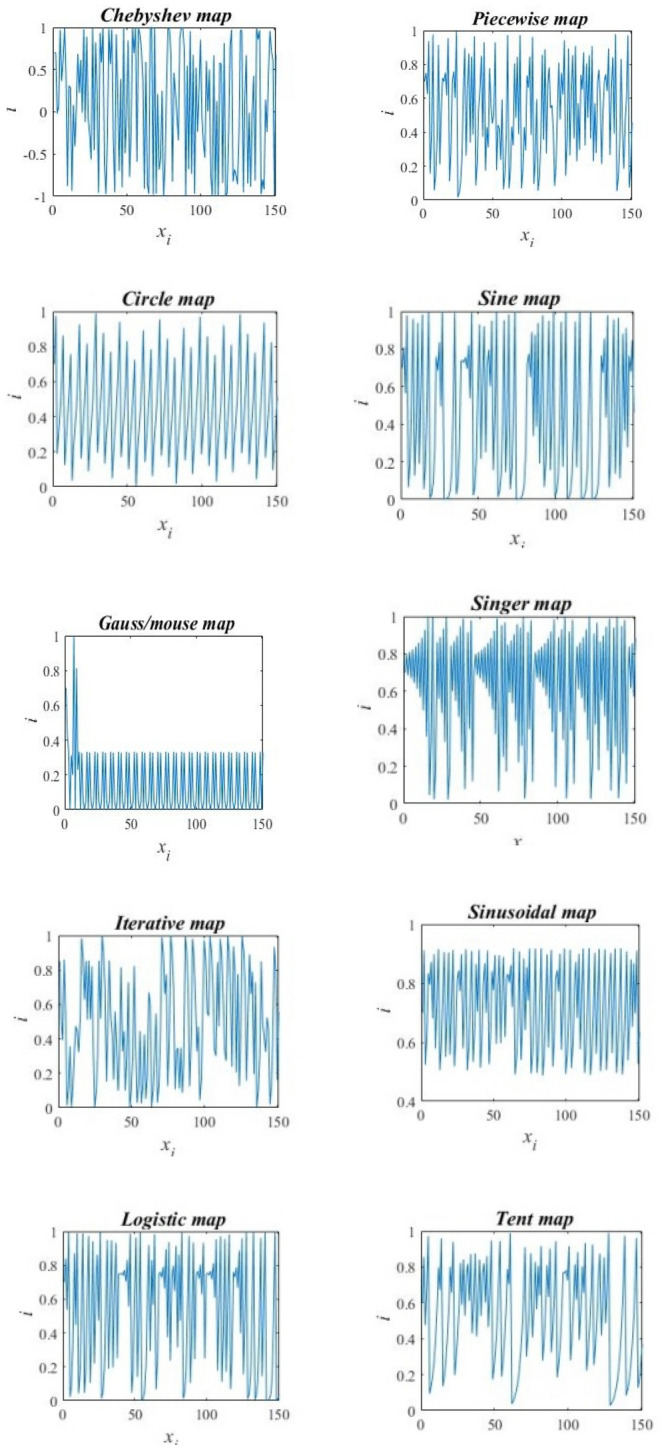
Ten chaotic maps.
The proposed CDMO for feature selection
In this study, an alternative feature selection technique is proposed using the Chaotic Dwarf Mongoose Optimization (CDMO) as in Fig. 2. Random numbers which are used in Eq. (7) are replaced by chaotic maps to avoid returning to same sleeping mound.
| 8 |
where is value obtained from well-known chaotic maps which reported in Table 1.
Figure 2.

Flowchart of the proposed CDMO algorithm.
Table 1.
Ten chaotic maps.
| #Map | Name | Definition | Range |
|---|---|---|---|
| 1 | Chebyshev | (-1,1) | |
| 2 | Circle | (0,1) | |
| 3 | Gauss/mouse | (0,1) | |
| 4 | Iterative | (-1,1) | |
| 5 | Logistic | (0,1) | |
| 6 | Piecewise | (0,1) | |
| 7 | Sine | (0,1) | |
| 8 | Singer | (0,1) | |
| 9 | Sinusoidal | (0,1) | |
| 10 | Tent | (0,1) |
After that, we have set the dimension of the problem, which is d in Eq. (1) as the number of features then give value of and in Eq. (2) as 0 and 1, respectively. For each row in Eq. (1) (i.e., the position of each element in ) is threshold by 0.5, since the values are set between 0 and 1. After that, elements with positions > 0.5 are considered as candidate features, while elements with positions < 0.5 are not considered in this solution.
| 9 |
The candidate features are then applied to the fitness function which calculates the classification accuracy of k-nearest neighbor classifier using the applied candidate features.
| 10 |
Each time the fitness function is invoked the dataset is divided using the holdout method to 80% training dataset and 20% testing dataset. Algorithm 1 and Fig. 2 show the algorithm and the flowchart of the proposed technique, respectively.

Algorithm 1 Steps of the developed method.
Experimental results
Dataset and parameters setting
Table 2 lists the 10 datasets that were used in this study which are come from the well-known UCI data warehouse33. They have been chosen with different dimensions and different patterns to evaluate the performance of the proposed method on several complexities.
Table 2.
Datasets used in this study.
| Index | Dataset | # dims | # instances |
|---|---|---|---|
| 1 | base_BreastEW | 30 | 569 |
| 2 | base_Exactly | 13 | 1000 |
| 3 | base_M-of-n3 | 13 | 1000 |
| 4 | breastEW | 30 | 569 |
| 5 | CongressEW | 16 | 435 |
| 6 | Ionosphere | 34 | 351 |
| 7 | KrvskpEW | 36 | 3196 |
| 8 | SonarEW | 60 | 208 |
| 9 | SpectEW | 22 | 267 |
| 10 | WaveformEW | 40 | 5000 |
K-nearest neighbor (KNN) is employed as a classifier in this study as it is one of the most common and simplest learning algorithms, it is trained using the training dataset, then, tested using the testing part, which ensures higher reliability. To simplify the evaluation process, we choose K = 5 in KNN as 5NN34.
Performance metrics
In this study we have used two types of metrics to evaluate the performance which are Fitness metrics and classification Metrics.
In fitness metrics we have used four statistical measurements which are the worst, best, mean fitness value and the standard deviation which are mathematically defined as following
| 11 |
| 12 |
| 13 |
| 14 |
where BS is the best score gained in each iteration and Nr is the number of runs35.
The second evaluation was used to evaluate the selected features using classification measures. These measures are accuracy, precision, sensitivity, specificity, and F-Score. Accuracy is a common technique of evaluation, which is defined as the ratio of correctly classified samples to all samples. It’s mathematically defined as following
| 15 |
Precision, specificity and sensitivity are proper metrics to measure the performance of classification across unbalanced datasets. While they are not affected by differences in data distribution, therefore these measures are useful for evaluating classification performance in unbalanced learning scenarios36. The F-Score metric make combination between precision and sensitivity and it is given by Eq. (19). Therefore, F-Score is suitable in unbalanced scenarios than the accuracy metric. Precision, sensitivity, specificity and F-score measures are defined by the following equations:
| 16 |
| 17 |
| 18 |
| 19 |
where TP is the true positive, FP is the false positive, FN is the false negative and TN represents the true negative.
Performance of DMO based on ten chaotic maps
To evaluate the performance of the proposed CDMO, 10 different datasets from UCI repository are used. The obtained results are compared with the DMO and other well-known meta-heuristic algorithms namely, PSO5, ACO6, ARO37, HHO38, EO39, RTHS40, RSGW41, SSAPSO42, BGA43 and WOA14 algorithms. Each one of them has been performed 25 runs in the same PC specifications. To test the convergence capability, the average 25 runs has been computed and compared for each algorithm. Table 3 illustrates the parameter settings of the algorithms used in this study. The experiments are divided into two sections, the first one is to evaluate the performance of the ten chaotic maps on DMO algorithm as shown in Tables 4 and 5, the second experiments are to compare the best chaotic maps with the six meta-heuristic algorithms DMO, ACO, PSO, ARO, HHO, and WOA as shown in Tables 6 and 7.
Table 3.
Parameter setting.
| Parameter | Value |
|---|---|
| k-value of KNN | 5 |
| Number of populations | 20 |
| Number of iterations | 100 |
| Problem dimensions | Number of features in the used dataset |
| Data search domain | [0 1] |
| Repetition of runs | 25 |
| No of babysitters in DMO | 3 |
| No of peep in DMO | 2 |
| α | 1 |
| τ | 1 |
| β | 0.1 |
| Pheromone in PSO | 0.2 |
| B constant in WOA | 1 |
| Initial value of chaotic | 0.7 |
| Iteration number in chaotic | 500 |
Table 4.
Accuracy comparison between ten CDMO.
| Accuracy | ||||||||||
|---|---|---|---|---|---|---|---|---|---|---|
| CDMO1 | CDMO2 | CDMO3 | CDMO4 | CDMO5 | CDMO6 | CDMO7 | CDMO8 | CDMO9 | CDMO10 | |
| base_exactly | 1 | 1 | 1 | 1 | 1 | 1 | 1 | 1 | 1 | 1 |
| base_BreastEW | 1 | 0.9911 | 0.9911 | 0.9823 | 0.9734 | 0.9734 | 0.9911 | 0.9911 | 0.9823 | 1 |
| base_M-of-n3 | 1 | 1 | 1 | 1 | 1 | 1 | 1 | 1 | 1 | 1 |
| breastEW | 0.9911 | 0.9823 | 0.9911 | 0.9911 | 0.9911 | 0.9823 | 0.9906 | 0.9921 | 0.9911 | 0.9646 |
| KrvskpEW | 0.9921 | 0.9874 | 0.9906 | 0.9859 | 0.9874 | 0.9859 | 1 | 0.9890 | 0.9843 | 0.9843 |
| SonarEW | 1 | 1 | 0.9268 | 1 | 1 | 0.9756 | 0.9056 | 1 | 1 | 0.9756 |
| SpectEW | 0.9622 | 0.9622 | 0.9622 | 0.9056 | 0.9622 | 0.8867 | 0.9065 | 0.9722 | 0.9433 | 0.9622 |
| Waveform | 0.9042 | 0.9077 | 0.8898 | 0.9058 | 0.9116 | 0.8993 | 0.9885 | 0.9192 | 0.9016 | 0.9109 |
| CongressEW | 0.9770 | 0.9655 | 0.9655 | 1 | 0.9885 | 0.9770 | 0.9885 | 1 | 0.9885 | 0.9885 |
| Ionosphere | 0.9714 | 0.9714 | 0.9428 | 0.9428 | 0.9557 | 0.9285 | 0.9871 | 0.9571 | 0.9428 | 0.9428 |
Significant values are in bold.
Table 5.
Average fitness comparison between ten CDMO.
| Average | ||||||||||
|---|---|---|---|---|---|---|---|---|---|---|
| CDMO1 | CDMO2 | CDMO3 | CDMO4 | CDMO5 | CDMO6 | CDMO7 | CDMO8 | CDMO9 | CDMO10 | |
| base_exactly | 0.0245 | 0.0264 | 0.0204 | 0.0129 | 0.0197 | 0.0331 | 0.0096 | 0.0055 | 0.0074 | 0.0234 |
| base_BreastEW | 0.0072 | 0.0112 | 0.0103 | 0.0215 | 0.0322 | 0.0334 | 0.0138 | 0.0095 | 0.0186 | 0.0027 |
| base_M-of-n3 | 0.0085 | 0.0085 | 0.0036 | 0.0012 | 0.0063 | 0.0012 | 0.0016 | 0.0016 | 0.0037 | 0.0071 |
| breastEW | 0.0123 | 0.0230 | 0.0105 | 0.0184 | 0.0107 | 0.0201 | 0.0157 | 0.0101 | 0.0160 | 0.0392 |
| KrvskpEW | 0.0137 | 0.0193 | 0.0128 | 0.0168 | 0.0190 | 0.0175 | 0.02 | 0.0131 | 0.0182 | 0.0219 |
| SonarEW | 0.0136 | 0.0139 | 0.1026 | 0.0065 | 0.0097 | 0.0441 | 0.0988 | 0.0058 | 0.0173 | 0.0473 |
| SpectEW | 0.0567 | 0.0490 | 0.0379 | 0.0958 | 0.0437 | 0.1137 | 0.0989 | 0.0588 | 0.0622 | 0.0511 |
| Waveform | 0.1016 | 0.0966 | 0.1139 | 0.0991 | 0.1004 | 0.1093 | 0.0122 | 0.0925 | 0.1012 | 0.0944 |
| CongressEW | 0.0248 | 0.0386 | 0.0345 | 0.0043 | 0.0140 | 0.0247 | 0.0122 | 0.0010 | 0.0167 | 0.0114 |
| Ionosphere | 0.0448 | 0.0307 | 0.0642 | 0.0747 | 0.0297 | 0.0927 | 0.0481 | 0.0612 | 0.0708 | 0.0667 |
Significant values are in bold.
Table 6.
Comparison between CDMO8 and 6 meta-heuristic algorithms in classification metrics.
| Accuracy | Precision | |||||||||||||
|---|---|---|---|---|---|---|---|---|---|---|---|---|---|---|
| ACO | PSO | WOA | DMO | ARO | HHO | CDMO8 | ACO | PSO | WOA | DMO | ARO | HHO | CDMO8 | |
| base_exactly | 0.9796 | 0.9126 | 0.8372 | 1 | 0.98 | 0.745 | 1 | 0.9811 | 0.9266 | 0.8559 | 1 | 0.9212 | 0.9259 | 1 |
| base_BreastEW | 0.9823 | 0.9869 | 0.9823 | 0.9876 | 0.9883 | 0.97345 | 0.9911 | 0.9823 | 0.9869 | 0.9823 | 0.9876 | 0.9838 | 0.9852 | 0.9911 |
| base_M-of-n3 | 0.9952 | 0.9748 | 0.9691 | 1 | 1 | 0.985 | 1 | 0.9952 | 0.9748 | 0.9691 | 1 | 0.9797 | 0.9809 | 1 |
| BreastEW | 0.9855 | 0.9837 | 0.9767 | 0.9911 | 0.9883 | 0.95575 | 0.9921 | 0.9850 | 0.9875 | 0.9771 | 0.9912 | 0.9832 | 0.9848 | 0.9861 |
| KrvskpEW | 0.9748 | 0.9744 | 0.9721 | 0.9894 | 0.9874 | 0.97026 | 0.9890 | 0.9777 | 0.9693 | 0.9744 | 0.9910 | 0.9738 | 0.9771 | 0.9939 |
| SonarEW | 0.9375 | 0.9619 | 0.9247 | 0.9824 | 0.9834 | 0.87804 | 1 | 0.9385 | 0.9679 | 0.9259 | 0.9855 | 0.9441 | 0.9559 | 1 |
| SpectEW | 0.9003 | 0.9116 | 0.8883 | 0.9198 | 0.9.32 | 0.94339 | 0.9722 | 0.9269 | 0.9336 | 0.9199 | 0.8373 | 0.9268 | 0.9044 | 1 |
| Waveform | 0.8562 | 0.8637 | 0.8556 | 0.9069 | 0.8227 | 0.802 | 0.9192 | 0.8812 | 0.8881 | 0.8810 | 0.9107 | 0.8834 | 0.8908 | 0.9188 |
| CongressEW | 0.9711 | 0.9766 | 0.9731 | 0.9880 | 09,839 | 0.95402 | 1 | 0.9524 | 0.9584 | 0.9584 | 0.9925 | 0.9564 | 0.9664 | 1 |
| Ionosphere | 0.9554 | 0.9308 | 0.9354 | 0.9434 | 0.96 | 0.92 | 0.9571 | 0.9511 | 0.9171 | 0.9203 | 0.9272 | 0.9295 | 0.9235 | 0.9565 |
| Sensitivity | Specificity | |||||||||||||
|---|---|---|---|---|---|---|---|---|---|---|---|---|---|---|
| ACO | PSO | WOA | DMO | ARO | HHO | CDMO8 | ACO | PSO | WOA | DMO | ARO | HHO | CDMO8 | |
| base_exactly | 0.9901 | 0.9529 | 0.9282 | 1 | 0.9678 | 0.9622 | 1 | 0.9566 | 0.8233 | 0.6374 | 1 | 0.9094 | 0.8964 | 1 |
| base_BreastEW | 0.9702 | 0.9761 | 0.9702 | 0.9943 | 0.9777 | 0.9796 | 0.9859 | 0.9894 | 0.9932 | 0.9894 | 0.9761 | 0.9794 | 0.9873 | 1 |
| base_M-of-n3 | 0.9939 | 0.9630 | 0.9506 | 1 | 0.9768 | 0.9726 | 1 | 0.9958 | 0.9816 | 0.9799 | 1 | 0.995 | 0.9908 | 1 |
| BreastEW | 0.9761 | 0.9685 | 0.9603 | 0.9947 | 0.9749 | 0.9746 | 1 | 0.9911 | 0.9926 | 0.9865 | 0.9837 | 0.9844 | 0.9894 | 0.9761 |
| KrvskpEW | 0.9697 | 0.9777 | 0.9672 | 0.9887 | 0.9758 | 0.9774 | 0.9849 | 0.9796 | 0.9714 | 0.9766 | 0.9901 | 0.9867 | 0.9792 | 0.9934 |
| SonarEW | 0.9472 | 0.9618 | 0.9375 | 0.9768 | 0.9558 | 0.9580 | 1 | 0.9263 | 0.9621 | 0.9100 | 0.9872 | 0.9679 | 0.9521 | 1 |
| SpectEW | 0.9504 | 0.9580 | 0.9428 | 0.7765 | 0.9069 | 0.8961 | 0.8181 | 0.7090 | 0.7345 | 0.68 | 0.9573 | 0.888 | 0.7772 | 1 |
| Waveform | 0.9045 | 0.9087 | 0.9039 | 0.8991 | 0.9040 | 0.9039 | 0.9218 | 0.7618 | 0.7758 | 0.7612 | 0.9145 | 0.8762 | 0.8046 | 0.9166 |
| CongressEW | 0.9781 | 0.9831 | 0.9738 | 0.9880 | 0.9807 | 0.9814 | 1 | 0.9726 | 0.9726 | 0.9727 | 0.9881 | 0.9843 | 0.9765 | 1 |
| Ionosphere | 0.9822 | 0.9831 | 0.9866 | 0.9911 | 0.9857 | 0.9866 | 0.9777 | 0.9072 | 0.8368 | 0.8432 | 0.8576 | 0.854 | 0.8660 | 0.92 |
| F-measure | ||||||||||||||
|---|---|---|---|---|---|---|---|---|---|---|---|---|---|---|
| ACO | PSO | WOA | DMO | ARO | HHO | CDMO8 | ||||||||
| base_exactly | 0.9854 | 0.9390 | 0.8890 | 1 | 0.9845 | 0.95783 | 1 | |||||||
| base_BreastEW | 0.9760 | 0.9822 | 0.9760 | 0.9901 | 0.9993 | 0.98847 | 0.9929 | |||||||
| base_M-of-n3 | 0.9934 | 0.9652 | 0.9576 | 1 | 1 | 0.98587 | 1 | |||||||
| BreastEW | 0.9804 | 0.9778 | 0.9684 | 0.9929 | 0.9865 | 0.98260 | 0.9930 | |||||||
| KrvskpEW | 0.9736 | 0.9734 | 0.9707 | 0.9898 | 0.9838 | 0.98143 | 0.9894 | |||||||
| SonarEW | 0.9419 | 0.9645 | 0.9303 | 0.9808 | 0.9782 | 0.96310 | 1 | |||||||
| SpectEW | 0.9380 | 0.9451 | 0.9304 | 0.7963 | 0.9455 | 0.89073 | 0.90 | |||||||
| Waveform | 0.8927 | 0.8982 | 0.8922 | 0.9047 | 0.8952 | 0.89737 | 0.9203 | |||||||
| CongressEW | 0.9680 | 0.9700 | 0.9655 | 0.9902 | 0.9830 | 0.97957 | 1 | |||||||
| Ionosphere | 0.9660 | 0.9485 | 0.9517 | 0.9577 | 0.9698 | 0.95973 | 0.9670 | |||||||
Significant values are in bold.
Table 7.
Comparison between CDMO8 and 6 meta-heuristic algorithms in fitness metrics.
| Average | Best | |||||||||||||
|---|---|---|---|---|---|---|---|---|---|---|---|---|---|---|
| ACO | PSO | WOA | DMO | ARO | HHO | CDMO8 | ACO | PSO | WOA | DMO | ARO | HHO | CDMO8 | |
| base_exactly | 0.0811 | 0.0995 | 0.1738 | 0.0125 | 0.0214 | 0.1181 | 0.0055 | 0.0204 | 0.0874 | 0.1627 | 0.0125 | 0.002 | 0.0708 | 0.0264 |
| base_BreastEW | 0.0202 | 0.0141 | 0.0181 | 0.0153 | 0.0149 | 0.0174 | 0.0095 | 0.0176 | 0.0116 | 0.0176 | 0.0123 | 0.0116 | 0.0148 | 0.0088 |
| base_M-of-n3 | 0.0200 | 0.0280 | 0.0365 | 0.0085 | 0.0025 | 0.0281 | 0.0016 | 0.0048 | 0.0252 | 0.0308 | 0.0085 | 0 | 0.0173 | 0.0016 |
| BreastEW | 0.0168 | 0.0178 | 0.0244 | 0.0127 | 0.0151 | 0.0196 | 0.0101 | 0.0144 | 0.0162 | 0.0232 | 0.0088 | 0.0116 | 0.0157 | 0.0088 |
| KrvskpEW | 0.0274 | 0.0268 | 0.0286 | 0.0165 | 0.0187 | 0.0276 | 0.0131 | 0.0251 | 0.0255 | 0.0278 | 0.0105 | 0.0125 | 0.0222 | 0.0109 |
| SonarEW | 0.0735 | 0.0457 | 0.0778 | 0.0371 | 0.0309 | 0.0656 | 0.0058 | 0.0624 | 0.0351 | 0.0752 | 0.0175 | 0.0165 | 0.0476 | 0.0139 |
| SpectEW | 0.1076 | 0.0891 | 0.1133 | 0.0881 | 0.0938 | 0.1033 | 0.0588 | 0.0989 | 0.0853 | 0.1117 | 0.0802 | 0.0867 | 0.094 | 0.0377 |
| Waveform | 0.1453 | 0.1392 | 0.1458 | 0.0997 | 0.1870 | 0.1434 | 0.0925 | 0.1438 | 0.1361 | 0.1444 | 0.0930 | 0.1772 | 0.1293 | 0.0807 |
| CongressEW | 0.0997 | 0.0997 | 0.0278 | 0.0146 | 0.0179 | 0.0757 | 0.0010 | 0.0226 | 0.0226 | 0.0268 | 0.0120 | 0.0160 | 0.021 | 0.0010 |
| Ionosphere | 0.0551 | 0.0698 | 0.0671 | 0.0686 | 0.0532 | 0.064 | 0.0612 | 0.0446 | 0.0657 | 0.0646 | 0.0566 | 0.04 | 0.0579 | 0.0429 |
| Worst | SD | |||||||||||||
|---|---|---|---|---|---|---|---|---|---|---|---|---|---|---|
| ACO | PSO | WOA | DMO | ARO | HHO | CDMO8 | ACO | PSO | WOA | DMO | ARO | HHO | CDMO8 | |
| base_exactly | 0.2478 | 0.219 | 0.2435 | 0.3175 | 0.2528 | 0.2561 | 0.29 | 0.0708 | 0.0289 | 0.0214 | 0.0491 | 0.0553 | 0.0252 | 0.1858 |
| base_BreastEW | 0.0332 | 0.029 | 0.0251 | 0.0297 | 0.0336 | 0.0301 | 0.0265 | 0.0034 | 0.0038 | 0.0014 | 0.0040 | 0.0054 | 0.0026 | 0.0034 |
| base_M-of-n3 | 0.0952 | 0.0936 | 0.0775 | 0.095 | 0.0788 | 0.088 | 0.03 | 0.0218 | 0.0105 | 0.0116 | 0.0209 | 0.0117 | 0.0111 | 0.0116 |
| BreastEW | 0.0302 | 0.0297 | 0.0328 | 0.0299 | 0.0336 | 0.0312 | 0.0354 | 0.0034 | 0.0028 | 0.0024 | 0.0051 | 0.0048 | 0.0026 | 0.0055 |
| KrvskpEW | 0.0394 | 0.04047 | 0.0368 | 0.0518 | 0.0539 | 0.0445 | 0.0203 | 0.0033 | 0.0031 | 0.0017 | 0.0081 | 0.0095 | 0.0024 | 0.0029 |
| SonarEW | 0.1317 | 0.1034 | 0.0976 | 0.1015 | 0.0985 | 0.1065 | 0.0488 | 0.0154 | 0.0146 | 0.0054 | 0.0201 | 0.0206 | 0.01 | 0.0130 |
| SpectEW | 0.1381 | 0.1102 | 0.1245 | 0.1195 | 0.1283 | 0.1241 | 0.1132 | 0.0089 | 0.0056 | 0.0032 | 0.0098 | 0.0103 | 0.0044 | 0.0136 |
| Waveform | 0.1599 | 0.1585 | 0.1594 | 0.1334 | 0.2337 | 0.169 | 0.1378 | 0.0028 | 0.0045 | 0.0031 | 0.0084 | 0.0130 | 0.0038 | 0.012 |
| CongressEW | 0.0421 | 0.0421 | 0.0374 | 0.0349 | 0.0372 | 0.0387 | 0.0345 | 0.0042 | 0.0042 | 0.0024 | 0.0048 | 0.0042 | 0.0033 | 0.0061 |
| Ionosphere | 0.0971 | 0.0977 | 0.0914 | 0.1149 | 0.1034 | 0.1009 | 0.1143 | 0.0134 | 0.0071 | 0.0059 | 0.0138 | 0.0175 | 0.0065 | 0.0128 |
Significant values are in bold.
Table 4 shows the accuracy of the average runs for the ten CDMO where the number after CDMO refers to the map number in Table 1, for example CDMO1 is Chebyshev map. Results in Table 4 shows that the Singer map which is CDMO8 has higher results in three datasets named (breastEW, SpectEW, Waveform), CDMO1 and CDMO7 have best results in (KrvskpEW) and (Ionosphere), respectively. All maps have same accuracy in two datasets named (base_exactly) and (base_M-of-n3). Table 5 shows the comparison of average fitness value of the ten chaotic maps. The Singer map (CDMO8) achieved best results in 5 out of 10 datasets. Both CDMO4 and CDMO6 achieved same result in base_M-of-n3. Also, CDMO1, CDMO3, CDMO5, CDMO7, CDMO10 have best results in one dataset for each, so CDMO8 has been chosen to be compared with ACO, PSO, WOA, ARO, HHO and DMO algorithms.
Figure 3 illustrates the convergence curves for the ten chaotic maps. In this figure, the number of iterations is equal to 100. As it can be observed from this figure, almost singer map obtains best result. This is due to that it converges faster than other maps.
Figure 3.


Comparison between ten chaotic maps.
Comparison with other meta-heuristic techniques
In this section, we will compare the performance of the developed method based on Singer map with well-known and most used techniques named PSO, ACO, ARO, HHO and WOA.
From Table 6, the CDMO gives best accuracy in seven datasets (base_BreastEW, SonarEW, SpectEW, Waveform, CongressEW, breastEW and Ionosphere) while DMO gives superior performance in one data set named KrvskpeEW. Moreover, DMO and CDMO give equal performance in 2 datasets (base_M-of-n3 and base_exactly). Based on the results of Precision, CDMO8 has better results in seven datasets. Whereas DMO has better results in one dataset named BreastEW, both CDMO8 and DMO have same results in two datasets. By analysis of the obtained results of the Sensitivity, the CDMO8 has highest results of four datasets, while DMO and PSO have highest results in three datasets and one dataset, respectively. Moreover, both CDMO8 and DMO have same results in two datasets named base_exactly and base_M-of-n3. For specificity results, CDMO8 has highest results in seven datasets while PSO has best results in only one dataset named BreastEW. Besides, both CDMO8 and DMO have same results in two datasets. In addition, F-measure results show that CDMO8 has better results in five datasets while DMO has better result in KrvskpEW dataset and ARO has better result in SpectEW and ionosphere datasets, both CDMO8 and DMO have same results in two datasets.
Table 7 presents the results of fitness metrics which is standard deviation SD, Best, Worst and the Average of fitness function. In the average of fitness function, the CDMO8 achieved best results in 9 out of 10 datasets while ACO has best results in Ionosphere dataset only. In terms of best measure, the CDMO8 has best results in 5 out 10 datasets while the original DMO has best results in 2 out of 10 datasets, ARO has better value in ionosphere and base_M-of-n3 datasets both CDMO8 and DMO have same results in breastEW dataset. Furthermore, for Worst measure, CDMO8 has best results in 5 out of 10 datasets, while PSO has the second rank by 3 out of 10 datasets. WOA and DMO have highest results in one dataset for each. Additionally concerning standard deviation, WOA has the superior results by 7 out of 10 datasets, neither CDMO nor original DMO got best results in standard deviation results.
Figure 4 shows the comparison between CDMO8 and other meta-heuristic algorithms (i.e., PSO, ACO, DMO, ARO, HHO and WOA) in convergence curve. As observed from figure, CDMO8 converges faster in most figures.
Figure 4.


Comparison between best chaotic map and 6 meta-heuristic algorithms.
Table 8 compares the accuracy of CDMO8 against 6 state-of-the-art methods namely, BGA, RTHS, RSGW, EO, SSAPSO and HSGW. It is clear that our proposed CDMO method stands at the top over these methods. CDMO8 produces higher accuracy in 8 out 10 datasets.
Table 8.
Comparison of CDMO8 with other 6 state-of-the-art methods based on achieved accuracy (highest classification accuracies are in bold).
| Dataset | Accuracy | ||||||
|---|---|---|---|---|---|---|---|
| BGA | RTHS | RSGW | EO | SSAPSO | HSGW | CDMO8 | |
| base_exactly | 1 | 0.997 | 0.997 | 0.75 | 0.967 | 1 | 1 |
| base_BreastEW | 0.9743 | 0.971 | 0.971 | 0.9857 | 0.95 | 0.986 | 0.9911 |
| base_M-of-n3 | 1 | 1 | 1 | 0.845 | 0.978 | 1 | 1 |
| BreastEW | 0.9754 | 098.2 | 0.982 | 0.9561 | 0.9755 | 0.981 | 0.9921 |
| KrvskpEW | 0.985 | 0.973 | 0.973 | 0.8435 | 0.951 | 0.973 | 0.9890 |
| SonarEW | 0.9904 | 1 | 0979 | 0.9048 | 0.9566 | 0.964 | 1 |
| SpectEW | 0.8955 | 0.9815 | 0.815 | 0.8703 | 0.7913 | 0.862 | 0.9722 |
| Waveform | 0.7836 | 0.841 | 0.757 | 0.788 | 0.9620 | 0.748 | 0.9192 |
| CongressEW | 0.9679 | 1 | 0.961 | 0.977 | 0.9686 | 0.975 | 1 |
| Ionosphere | 0.9489 | 1 | 0.978 | 0.9571 | 0.98 | 0.944 | 0.9571 |
Performance evaluation on CEC’22 benchmark functions
In this section, the performance of the proposed CDMO algorithm in solving optimization problems is tested. To this end, the numerical solving efficiency of CDMO is evaluated by solving twelve functions of CEC’22. The performance of the proposed CDMO on the CEC’22 benchmark function has been determined. Table 9 presents the outcomes for a CEC’2022 test suite for 30 runs performed by the proposed ten chaotic DMO. These benchmark functions consist of four types unimodal, basic, hybrid and composite functions. It is found that CDMO9 achieves the best performance.
Table 9.
Comparison of simulation outcomes using DMO with 10 chaotic maps for a CEC’2022 test suite for 30 runs.
| Fun | CDMO1 | CDMO2 | CDMO3 | CDMO4 | CDMO5 | CDMO6 | CDMO7 | CDMO8 | CDMO9 | CDMO10 | |
|---|---|---|---|---|---|---|---|---|---|---|---|
| F1 | Mean | 37.6703 | 49.2258 | 55.2711 | 24.1597 | 38.7636 | 31.7829 | 41.1619 | 42.5261 | 44.4219 | 49.0182 |
| STD | − 27.0101 | − 25.142 | 1.4219 | − 15.2403 | − 19.8947 | − 2.752 | − 25.7849 | − 12.7627 | − 18.1099 | − 18.616 | |
| F2 | Mean | 71.3877 | 67.4698 | 72.7695 | 67.069 | 70.3485 | 70.0904 | 66.9872 | 67.4974 | 73.118 | 69.0384 |
| STD | 28.6156 | 31.3227 | 27.4624 | 31.5527 | 29.4815 | 29.5777 | 31.5268 | 31.3894 | 27.7238 | 30.1431 | |
| F3 | Mean | 47.8944 | 47.8966 | 47.8976 | 47.8987 | 47.8905 | 47.8964 | 47.8923 | 47.8925 | 47.8869 | 47.8999 |
| STD | 16.7706 | 16.77 | 16.7727 | 16.7707 | 16.7623 | 16.7719 | 16.7678 | 16.7747 | 16.7674 | 16.7748 | |
| F4 | Mean | 31.573 | 41.3039 | 18.9391 | 29.6284 | 32.9669 | 38.6676 | 39.858 | 22.6606 | 29.972 | 38.5803 |
| STD | − 13.2639 | 4.7712 | − 14.0327 | − 4.1446 | − 0.44749 | 4.0023 | − 7.8498 | − 10.5974 | − 8.3744 | 1.8914 | |
| F5 | Mean | 51.20491 | 46.35887 | 38.06082 | 35.40594 | 35.23488 | 39.40386 | 38.17021 | 58.53465 | 29.7295 | 32.53841 |
| STD | − 8.19181 | 0.523679 | − 2.8823 | 12.2422 | 1.414808 | − 10.4939 | − 0.67047 | − 10.3861 | − 13.7808 | 13.33265 | |
| F6 | Mean | 31.54436 | 39.09761 | 24.29382 | 23.30663 | 39.95076 | 34.20494 | 43.23234 | 31.10375 | 45.60005 | 29.90376 |
| STD | 1.002241 | − 5.60402 | − 14.5199 | 3.995714 | − 2.25021 | − 7.78239 | − 1.25563 | 4.310759 | − 5.67635 | − 2.97554 | |
| F7 | Mean | 34.85993 | 49.18917 | 36.43779 | 46.29711 | 25.4561 | 39.70633 | 30.87552 | 43.34505 | 42.17393 | 31.99279 |
| STD | − 3.56281 | − 6.69832 | − 7.64214 | 5.231094 | − 3.48243 | 2.88266 | − 5.48696 | − 1.65038 | − 14.488 | 1.675022 | |
| F8 | Mean | 40.14696 | 43.02149 | 37.50739 | 29.97309 | 45.87442 | 30.97324 | 43.92831 | 49.30015 | 43.53387 | 30.326 |
| STD | 4.511035 | 1.558652 | − 13.2439 | − 6.44802 | − 20.1744 | 7.831558 | 11.106 | − 5.7076 | − 6.19182 | − 14.092 | |
| F9 | Mean | 45.96478 | 37.75997 | 32.08481 | 44.69134 | 39.9951 | 40.51609 | 42.70853 | 31.55867 | 37.03655 | 42.32642 |
| STD | − 0.81111 | 5.822384 | − 1.66304 | 1.246249 | − 11.839 | − 14.2114 | − 11.8797 | − 3.09272 | − 10.0039 | − 2.42989 | |
| F10 | Mean | 38.10615 | 44.71744 | 39.21914 | 43.36055 | 29.22045 | 39.41734 | 34.92506 | 38.68287 | 43.13838 | 28.86259 |
| STD | − 16.5793 | − 0.82598 | − 0.61679 | − 0.3013 | 12.58064 | − 2.10653 | − 21.5561 | − 7.8547 | 3.256351 | 13.59188 | |
| F11 | Mean | 44.27529 | 35.29008 | 31.00094 | 23.31097 | 37.44925 | 30.37191 | 32.86412 | 34.95504 | 53.42543 | 41.02269 |
| STD | 3.133682 | 1.649913 | − 6.10969 | − 13.5542 | 3.761989 | − 11.6043 | − 12.9215 | − 5.83714 | 6.09463 | − 5.55082 | |
| F12 | Mean | − 12.6973 | 0.211765 | 6.528745 | − 3.575 | − 4.6557 | − 10.972 | − 12.2923 | − 12.2741 | 2.576182 | 6.86794 |
| STD | 37.70109 | 35.08934 | 36.39644 | 39.99058 | 30.95312 | 36.44769 | 36.40298 | 33.68914 | 46.62329 | 41.95957 |
In order to verify the effectiveness of CDMO9, the results of the proposed CDMO9 are compared, in Table 10, with six novel optimization algorithms namely, Artificial Hummingbird Algorithm (AHA)44, African Vultures Optimization Algorithm (AVOA)45, Crow Search Algorithm (CSA)46, Harris Hawks Optimization (HHO)38, Northern Goshawk Optimization (NGO)47 and Satin Bowerbird Optimizer (SBO)48. Besides, in order to demonstrate the ability of CDMO9 to solve optimization problems, the obtained results are compared with two algorithms recently improved by scholars namely, an adaptive quadratic interpolation and rounding mechanism Sine Cosine Algorithm (ARSCA)49 and boosting Archimedes Optimization Algorithm using trigonometric operators (SCAOA)50. The experimental results show that the proposed method compares favorably with these methods.
Table 10.
Comparison of simulation outcomes for a CEC’2022 test suite for 30 runs (highest classification accuracies are in bold).
| Fun | AHA | AVOA | CSA | HHO | NGO | SBO | ARSCA | SCAOA | CDMO9 | |
|---|---|---|---|---|---|---|---|---|---|---|
| F1 | Mean | 3.00E+02 | 3.00E+02 | 6.04E+03 | 3.00E+02 | 3.00E+02 | 3.00E+02 | 3.00E+02 | 3.23E+02 | 4.421E+01 |
| STD | 1.34E−11 | 7.24E−14 | 2.68E+03 | 1.36E−01 | 5.59E−14 | 2.13E−01 | 1.96E−02 | 1.79E+01 | − 1.810E+01 | |
| F2 | Mean | 4.07E+02 | 4.16E+02 | 6.10E+02 | 4.22E+02 | 4.04E+02 | 4.10E+02 | 4.05E+02 | 4.04E+02 | 7.311E+01 |
| STD | 1.76E+01 | 2.70E+01 | 9.44E+01 | 2.91E+01 | 1.30E+01 | 2.09E+01 | 1.31E+01 | 2.95E+00 | 2.772E+01 | |
| F3 | Mean | 6.00E+02 | 6.04E+02 | 6.28E+02 | 6.18E+02 | 6.00E+02 | 6.04E+02 | 6.04E+02 | 6.01E+02 | 4.788E+01 |
| STD | 9.71E−03 | 3.85E+00 | 6.14E+00 | 1.19E+01 | 1.94E−01 | 7.05E+00 | 3.31E+00 | 1.89E−01 | 1.676E+01 | |
| F4 | Mean | 8.23E+02 | 8.26E+02 | 8.35E+02 | 8.29E+02 | 8.09E+02 | 8.27E+02 | 8.20E+02 | 8.11E+02 | 2.997E+01 |
| STD | 7.64E+00 | 9.33E+00 | 9.63E+00 | 7.39E+00 | 2.86E+00 | 9.69E+00 | 6.29E+00 | 2.90E+00 | − 8.374E+00 | |
| F5 | Mean | 9.22E+02 | 1.03E+03 | 1.11E+03 | 1.38E+03 | 9.00E+02 | 1.33E+03 | 9.10E+02 | 9.00E+02 | 2.972E+01 |
| STD | 4.29E+01 | 1.14E+02 | 8.43E+01 | 2.07E+02 | 1.55E+00 | 2.72E+02 | 2.05E+01 | 2.01E−01 | − 1.378E+01 | |
| F6 | Mean | 2.05E+03 | 3.42E+03 | 3.41E+05 | 2.99E+03 | 1.97E+03 | 2.51E+03 | 3.53E+03 | 2.96E+03 | 4.560E+01 |
| STD | 4.79E+02 | 1.38E+03 | 1.07E+06 | 1.44E+03 | 2.24E+02 | 9.57E+02 | 1.94E+03 | 1.00E+03 | − 5.676E+00 | |
| F7 | Mean | 2.01E+03 | 2.03E+03 | 2.05E+03 | 2.03E+03 | 2.01E+03 | 2.05E+03 | 2.02E+03 | 2.02E+03 | 4.2173E+01 |
| STD | 9.42E+00 | 1.03E+01 | 1.48E+01 | 1.11E+01 | 6.67E+00 | 4.54E+01 | 8.10E+00 | 6.26E+00 | − 1.4488E+01 | |
| F8 | Mean | 2.22E+03 | 2.22E+03 | 2.23E+03 | 2.23E+03 | 2.22E+03 | 2.27E+03 | 2.22E+03 | 2.22E+03 | 4.353E+01 |
| STD | 6.78E+00 | 6.53E+00 | 4.53E+00 | 9.55E+00 | 8.82E+00 | 8.77E+01 | 6.91E+00 | 8.02E+00 | − 6.1912E+00 | |
| F9 | Mean | 2.53E+03 | 2.53E+03 | 2.65E+03 | 2.55E+03 | 2.53E+03 | 2.53E+03 | 2.53E+03 | 2.53E+03 | 3.7036E+01 |
| STD | 1.64E−10 | 9.11E+00 | 3.06E+01 | 5.08E+01 | 4.63E−13 | 2.68E+01 | 2.68E+01 | 7.08E+00 | − 1.0003E+01 | |
| F10 | Mean | 2.50E+03 | 2.50E+03 | 2.51E+03 | 2.61E+03 | 2.53E+03 | 2.69E+03 | 2.54E+03 | 2.51E+03 | 4.3138E+01 |
| STD | 1.17E−01 | 1.34E−01 | 8.11E+00 | 7.46E+01 | 4.67E+01 | 1.97E+02 | 5.78E+01 | 3.67E+01 | 3.256 E+00 | |
| F11 | Mean | 2.62E+03 | 2.64E+03 | 2.92E+03 | 2.80E+03 | 2.64E+03 | 2.74E+03 | 2.66E+03 | 2.61E+03 | 5.3425E+01 |
| STD | 8.07E+01 | 6.48E+01 | 8.71E+01 | 1.33E+02 | 7.75E+01 | 1.62E+02 | 1.31E+02 | 1.60E+01 | 6.094E+00 | |
| F12 | Mean | 2.87E+03 | 2.88E+03 | 2.89E+03 | 2.89E+03 | 2.86E+03 | 2.95E+03 | 2.87E+03 | 2.86E+03 | 2.5761E+00 |
| STD | 4.97E+00 | 8.90E+00 | 1.48E+01 | 2.61E+01 | 1.65E+00 | 5.33E+01 | 5.98E+00 | 1.34E+00 | 4.6623E+01 |
Conclusion and future work
Chaotic Dwarf Mongoose Optimization Algorithm (CDMO) was proposed which is Dwarf Mongoose algorithm hybridized by chaos. To enhance the performance of the proposed technique, ten chaotic maps were employed where CDMO is used as a wrapper feature selector. The CDMO gives superior performance than the well-known meta-heuristic algorithms, namely PSO, ACO, WOA, ARO, HHO BGA, RTHS, RSGW, EO, SSAPSO, HSGW and DMO. The obtained results proved that the capability of CDMO to select the best feature set gives high classification results. Moreover, the experimental results proved that the adjusted variable using the Singer map significantly enhanced the DMO algorithm in terms of classification performance, and fitness performance. Moreover, our proposed algorithm is tested using the recent optimizers in CEC’22.
In the future work we can extend this work to solve real world problem like medical data. In addition, it would be interested to investigate in hybridization DMO algorithm with another swarm meta-heuristic algorithm.
Ethics approval
This research contains neither human nor animal studies.
Author contributions
M.A.: software, investigation, formal analysis, visualization, writing—original draft, writing—review and editing. M.A.E.: conceptualization, methodology, data curation, validation, investigation, writing—original draft, writing—review and editing, visualization. A.H.E.-B.: methodology, software, data curation, investigation, formal analysis, validation, visualization, writing—review and editing, writing—original draft.
Funding
Open access funding provided by The Science, Technology & Innovation Funding Authority (STDF) in cooperation with The Egyptian Knowledge Bank (EKB).
Data availability
The datasets used in this study are available in the UC Irvine Machine Learning Repository, “https://archive.ics.uci.edu/: Access Date: 10 May 2023. “
Competing interests
The authors declare no competing interests.
Footnotes
Publisher's note
Springer Nature remains neutral with regard to jurisdictional claims in published maps and institutional affiliations.
References
- 1.Kyaw KS, Limsiroratana S, Sattayaraksa T. A comparative study of meta-heuristic and conventional search in optimization of multi-dimensional feature selection. Int. J. Appl. Metaheuristic Comput. (IJAMC) 2022;13(1):1–34. doi: 10.4018/IJAMC.292517. [DOI] [Google Scholar]
- 2.Hafez, A. I., Zawbaa, H. M., Emary, E., Mahmoud, H. A., & Hassanien, A. E. An innovative approach for feature selection based on chicken swarm optimization. In 2015 7th international conference of soft computing and pattern recognition (SoCPaR) pp 19–24. IEEE. 10.1109/SOCPAR.2015.7492775 (2015).
- 3.Emary E, Zawbaa HM. Feature selection via Lèvy Antlion optimization. Pattern Anal. Appl. 2019;22:857–876. doi: 10.1007/s10044-018-0695-2. [DOI] [Google Scholar]
- 4.Long W, Xu M, Jiao J, Wu T. A velocity-based butterfly optimization algorithm for high-dimensional optimization and feature selection. Expert Syst. Appl. 2022;201:117217. doi: 10.1016/j.eswa.2022.117217. [DOI] [Google Scholar]
- 5.Poli R, Kennedy J, Blackwell T. Particle swarm optimization: An overview. Swarm Intell. 2007;1:33–57. doi: 10.1007/s11721-007-0002-0. [DOI] [Google Scholar]
- 6.Dorigo M, Birattari M, Stutzle T. Ant colony optimization. IEEE Comput. Intell. Mag. 2006;1(4):28–39. doi: 10.1109/MCI.2006.329691. [DOI] [Google Scholar]
- 7.Sivanandam, S., & Deepa, S. Genetic Algorithm Optimization Problems. In: Introduction to Genetic Algorithms (Springer, Berlin, Heidelberg). 10.1007/978-3-540-73190-0_7 (2008).
- 8.Gandomi AH, Yang XS, Talatahari S, Alavi AH. Metaheuristic algorithms in modeling and optimization. Metaheuristic Appl. Struct. Infrastruct. 2013;1:1–24. [Google Scholar]
- 9.Nikolaev, A.G. & Jacobson, S.H. Simulated Annealing. In Handbook of Metaheuristics.146, (eds Gendreau, M. & Potvin, J.Y.) Int. Ser. Oper. Res. Manag. Sci.10.1007/978-1-4419-1665-5_1 (Springer, Boston, MA, 2010).
- 10.Hao, Z. F., Guo, G. H., & Huang, H. A particle swarm optimization algorithm with differential evolution. In 2007 international conference on machine learning and cybernetics, 2, 1031–1035. IEEE. 10.1109/ICMLC.2007.4370294 (2007).
- 11.Joshi AS, Kulkarni O, Kakandikar GM, Nandedkar VM. Cuckoo search optimization-a review. Mater. Today Proc. 2017;4(8):7262–7269. doi: 10.1016/j.matpr.2017.07.055. [DOI] [Google Scholar]
- 12.Afshinmanesh, F., Marandi, A., & Rahimi-Kian, A. A novel binary particle swarm optimization method using artificial immune system. In EUROCON 2005-The International Conference on" Computer as a Tool”, 1, 217–220. IEEE.10.1109/EURCON.2005.1629899 (2005).
- 13.Shen Q, Shi WM, Kong W. Hybrid particle swarm optimization and tabu search approach for selecting genes for tumor classification using gene expression data. Comput. Biol. Chem. 2008;32(1):53–60. doi: 10.1016/j.compbiolchem.2007.10.001. [DOI] [PubMed] [Google Scholar]
- 14.Nasiri J, Khiyabani FM. A whale optimization algorithm (WOA) approach for clustering. Cogent Math. Stat. 2018;5(1):1483565. doi: 10.1080/25742558.2018.1483565. [DOI] [Google Scholar]
- 15.Dokeroglu T, Deniz A, Kiziloz HE. A comprehensive survey on recent metaheuristics for feature selection. Neurocomputing. 2022 doi: 10.1016/j.neucom.2022.04.083. [DOI] [Google Scholar]
- 16.Xue B, Zhang M, Browne WN. Particle swarm optimization for feature selection in classification: A multi-objective approach. IEEE Trans. Cybern. 2012;43(6):1656–1671. doi: 10.1109/TSMCB.2012.2227469. [DOI] [PubMed] [Google Scholar]
- 17.Emary E, Zawbaa HM, Hassanien AE. Binary ant lion approaches for feature selection. Neurocomputing. 2016;213:54–65. doi: 10.1016/j.neucom.2016.03.101. [DOI] [Google Scholar]
- 18.Aalaei S, Shahraki H, Rowhanimanesh A, Eslami S. Feature selection using genetic algorithm for breast cancer diagnosis: Experiment on three different datasets. Iran. J. Basic Med. Sci. 2016;19(5):476. [PMC free article] [PubMed] [Google Scholar]
- 19.Ferriyan, A., Thamrin, A. H., Takeda, K., & Murai, J. Feature selection using genetic algorithm to improve classification in network intrusion detection system. In 2017 international electronics symposium on knowledge creation and intelligent computing (IES-KCIC) (pp. 46–49). IEEE (2017).
- 20.Karaboga D, Akay BA. A comparative study of artificial bee colony algorithm. Appl. Math. Comput. 2009;214(1):108–132. [Google Scholar]
- 21.Etminaniesfahani A, Gu H, Salehipour A. ABFIA: A hybrid algorithm based on artificial bee colony and Fibonacci indicator algorithm. J. Comput. Sci. 2022;61:101651. doi: 10.1016/j.jocs.2022.101651. [DOI] [Google Scholar]
- 22.Etminaniesfahani A, Ghanbarzadeh A, Marashi Z. Fibonacci indicator algorithm: A novel tool for complex optimization problems. Eng. Appl. Artif. Intell. 2018;74:1–9. doi: 10.1016/j.engappai.2018.04.012. [DOI] [Google Scholar]
- 23.Akinola OA, Ezugwu AE, Oyelade ON, Agushaka JO. A hybrid binary dwarf mongoose optimization algorithm with simulated annealing for feature selection on high dimensional multi-class datasets. Sci. Rep. 2022;12(1):14945. doi: 10.1038/s41598-022-18993-0. [DOI] [PMC free article] [PubMed] [Google Scholar]
- 24.Eluri RK, Devarakonda N. Binary golden eagle optimizer with time-varying flight length for feature selection. Knowl. Based Syst. 2022;247:108771. doi: 10.1016/j.knosys.2022.108771. [DOI] [Google Scholar]
- 25.Eluri RK, Devarakonda N. Chaotic binary pelican optimization algorithm for feature selection. Int. J. Uncert. Fuzziness Knowl. Based Syst. 2023;31(03):497–530. doi: 10.1142/S0218488523500241. [DOI] [Google Scholar]
- 26.Eluri RK, Devarakonda N. Feature selection with a binary flamingo search algorithm and a genetic algorithm. Multimed. Tools Appl. 2023;82(17):26679–26730. doi: 10.1007/s11042-023-15467-x. [DOI] [Google Scholar]
- 27.Agushaka JO, Ezugwu AE, Abualigah L. Dwarf mongoose optimization algorithm. Comput. Methods Appl. Mech. Eng. 2022;391:114570. doi: 10.1016/j.cma.2022.114570. [DOI] [Google Scholar]
- 28.Yang D, Li G, Cheng G. On the efficiency of chaos optimization algorithms for global optimization. Chaos Solit. Fractals . 2007;34(4):1366–1375. doi: 10.1016/j.chaos.2006.04.057. [DOI] [Google Scholar]
- 29.Chuang LY, Yang CH, Li JC. Chaotic maps based on binary particle swarm optimization for feature selection. Appl. Soft Comput. 2011;11(1):239–248. doi: 10.1016/j.asoc.2009.11.014. [DOI] [Google Scholar]
- 30.Sayed GI, Darwish A, Hassanien AE. A new chaotic whale optimization algorithm for features selection. J. Classif. 2018;35(2):300–344. doi: 10.1007/s00357-018-9261-2. [DOI] [Google Scholar]
- 31.Sayed GI, Tharwat A, Hassanien AE. Chaotic dragonfly algorithm: An improved metaheuristic algorithm for feature selection. Appl. Intell. 2019;49:188–205. doi: 10.1007/s10489-018-1261-8. [DOI] [Google Scholar]
- 32.Sayed GI, Hassanien AE, Azar AT. Feature selection via a novel chaotic crow search algorithm. Neural Comput. Appl. 2019;31:171–188. doi: 10.1007/s00521-017-2988-6. [DOI] [Google Scholar]
- 33.Frank, A., & Asuncion, A. UCI machine learning repository (2010).
- 34.Peterson LE. K-nearest neighbor. Scholarpedia. 2009;4(2):1883. doi: 10.4249/scholarpedia.1883. [DOI] [Google Scholar]
- 35.Derrac J, García S, Molina D, Herrera F. A practical tutorial on the use of nonparametric statistical tests as a methodology for comparing evolutionary and swarm intelligence algorithms. Swarm Evol. Comput. 2011;1(1):3–18. doi: 10.1016/j.swevo.2011.02.002. [DOI] [Google Scholar]
- 36.He H, Garcia EA. Learning from imbalanced data. IEEE Trans. Knowl. Data Eng. 2009;21(9):1263–1284. doi: 10.1109/TKDE.2008.239. [DOI] [Google Scholar]
- 37.Wang L, Cao Q, Zhang Z, Mirjalili S, Zhao W. Artificial rabbits optimization: A new bio-inspired meta-heuristic algorithm for solving engineering optimization problems. Eng. Appl. Artif. Intell. 2022;114:105082. doi: 10.1016/j.engappai.2022.105082. [DOI] [Google Scholar]
- 38.Heidari AA, Mirjalili S, Faris H, Aljarah I, Mafarja M, Chen H. Harris hawks optimization: Algorithm and applications. Future Gen. Comput. Syst. 2019;97:849–872. doi: 10.1016/j.future.2019.02.028. [DOI] [Google Scholar]
- 39.Ahmed S, Ghosh KK, Mirjalili S, Sarkar R. AIEOU: Automata-based improved equilibrium optimizer with U-shaped transfer function for feature selection. Knowl. Based Syst. 2021;228:107283. doi: 10.1016/j.knosys.2021.107283. [DOI] [Google Scholar]
- 40.Ahmed S, Ghosh KK, Singh PK, Geem ZW, Sarkar R. Hybrid of harmony search algorithm and ring theory-based evolutionary algorithm for feature selection. IEEE Access. 2020;8:102629–102645. doi: 10.1109/ACCESS.2020.2999093. [DOI] [Google Scholar]
- 41.Mafarja M, Qasem A, Heidari AA, Aljarah I, Faris H, Mirjalili S. Efficient hybrid nature-inspired binary optimizers for feature selection. Cognit Comput. 2020;12:150–175. doi: 10.1007/s12559-019-09668-6. [DOI] [Google Scholar]
- 42.Ibrahim RA, Ewees AA, Oliva D, Abd Elaziz M, Lu S. Improved salp swarm algorithm based on particle swarm optimization for feature selection. J. Ambient Intell. Hum. Comput. 2019;10:3155–3169. doi: 10.1007/s12652-018-1031-9. [DOI] [Google Scholar]
- 43.Leardi R. Application of a genetic algorithm to feature selection under full validation conditions and to outlier detection. J. Chemometr. 1994;8(1):65–79. doi: 10.1002/cem.1180080107. [DOI] [Google Scholar]
- 44.Zhao W, Wang L, Mirjalili S. Artificial hummingbird algorithm: A new bio-inspired optimizer with its engineering applications. Comput. Methods Appl. Mech. Eng. 2022;388:114194. doi: 10.1016/j.cma.2021.114194. [DOI] [Google Scholar]
- 45.Abdollahzadeh B, Gharehchopogh FS, Mirjalili S. African vultures optimization algorithm: A new nature-inspired metaheuristic algorithm for global optimization problems. Comput. Ind. Eng. 2021;158:107408. doi: 10.1016/j.cie.2021.107408. [DOI] [Google Scholar]
- 46.Askarzadeh A. A novel metaheuristic method for solving constrained engineering optimization problems: Crow search algorithm. Comput. Struct. 2016;169:1–12. doi: 10.1016/j.compstruc.2016.03.001. [DOI] [Google Scholar]
- 47.Dehghani M, Hubálovsky Š. Northern goshawk optimization: A new swarm-based algorithm for solving optimization problems. IEEE Access. 2021;9:162059–162080. doi: 10.1109/ACCESS.2021.3133286. [DOI] [Google Scholar]
- 48.Moosavi SHS, Bardsiri VK. Satin bowerbird optimizer: A new optimization algorithm to optimize anfis for software development effort estimation. Eng. Appl. Artif. Intell. 2017;60:1–15. doi: 10.1016/j.engappai.2017.01.006. [DOI] [Google Scholar]
- 49.Yang X, Wang R, Zhao D, Yu F, Huang C, Heidari AA, Cai Z, Bourouis S, Algarni AD, Chen H. An adaptive quadratic interpolation and rounding mechanism sine cosine algorithm with application to constrained engineering optimization problems. Expert Syst. Appl. 2023;213:119041. doi: 10.1016/j.eswa.2022.119041. [DOI] [Google Scholar]
- 50.Neggaz I, Neggaz N, Fizazi H. Boosting archimedes optimization algorithm using trigonometric operators based on feature selection for facial analysis. Neural Comput. Appl. 2023;35:3903–3923. doi: 10.1007/s00521-022-07925-8. [DOI] [PMC free article] [PubMed] [Google Scholar]
Associated Data
This section collects any data citations, data availability statements, or supplementary materials included in this article.
Data Availability Statement
The datasets used in this study are available in the UC Irvine Machine Learning Repository, “https://archive.ics.uci.edu/: Access Date: 10 May 2023. “