Generalizability of Deep Learning Classification of Spinal Osteoporotic Compression Fractures on Radiographs Using an Adaptation of the Modified-2 Algorithm-Based Qualitative Criteria

Abstract

Rationale and Objectives:

Spinal osteoporotic compression fractures (OCFs) can be an early biomarker for osteoporosis but are often subtle, incidental, and under-reported. To ensure early diagnosis and treatment of osteoporosis, we aimed to build a deep learning vertebral body classifier for OCFs as a critical component of our future automated opportunistic screening tool.

Materials and Methods:

We retrospectively assembled a local dataset including 1,790 subjects and 15,050 vertebral bodies (thoracic and lumbar). Each vertebral body was annotated using an adaption of the modified-2 algorithm-based qualitative criteria. The Osteoporotic Fractures in Men (MrOS) Study dataset provided thoracic and lumbar spine radiographs of 5,994 men from six clinical centers. Using both datasets, five deep learning algorithms were trained to classify each individual vertebral body of the spine radiographs. Classification performance was compared for these models using multiple metrics including the area under the receiver operating characteristic curve (AUC-ROC), sensitivity, specificity, and positive predictive value (PPV).

Results:

Our best model, built with ensemble averaging, achieved an AUC-ROC of 0.948 and 0.936 on the local dataset’s test set and the MrOS dataset’s test set, respectively. After setting the cutoff threshold to prioritize PPV, this model achieved a sensitivity of 54.5% and 47.8%, a specificity of 99.7% and 99.6%, and a PPV of 89.8% and 94.8%.

Conclusion:

Our model achieved an AUC-ROC >0.90 on both datasets. This testing shows some generalizability to real world clinical datasets and a suitable performance for a future opportunistic osteoporosis screening tool.

INTRODUCTION

Osteoporosis affects 9% of individuals over 50 years old in the US (1) and 200 million women globally (2). In developed countries, one out of three individuals will suffer an osteoporotic compression fracture (OCF) in their lifetime (2). After the first OCF, the risk for subsequent OCFs increases greatly (3–5). Even one OCF can decrease quality of life and increase risk of mortality (6).

Osteoporosis screening is evidence-based and is endorsed by many organizations, including the US Preventive Services Task Force, but remains underutilized. Between 2004 and 2006, more than 2/3 of women who should have been screened for osteoporosis were not (7). From 2006–2010, screening of US women with Medicare using dual-energy X-ray absorptiometry decreased by 56% (8). The rate of osteoporosis screening for high-risk men is also low (9).

Opportunistic osteoporosis screening, which uses pre-existing imaging to increase osteoporosis detection rates, can complement current osteoporosis screening methods and is desired to introduce minimum extra cost. Several approaches to opportunistic osteoporosis screening have been proposed (10–29). Many research groups used computerized tomography (CT) images (10–22), while few used radiographs (23–29). Radiography is a ubiquitous imaging modality used early in diagnostic workup of many conditions with an estimated 183 million exams in US hospitals in 2010 (30). Thus, using radiographs to conduct opportunistic osteoporosis screening is as important as using CT and could potentially reach a broader patient population. Using radiographs, Lee et al. (23) and Zhang et al. (24) used machine learning algorithms to estimate bone mineral density. However, using bone mineral density as a biomarker of osteoporosis detection has known limitations (31, 32). Spinal OCFs can serve as an additional osteoporosis biomarker and are often incidental on chest or abdominal images and frequently under-reported, resulting in under-diagnosis and under-treatment (33). Applying automated opportunistic OCF screening to existing imaging studies could result in earlier and more extensive osteoporosis identification and treatment. Multiple studies (25–29) have attempted to automatically detect OCFs using radiographs. However, these studies had limitations including single center data leading to possible overfitting (25–28) and unclear dataset construction processes (29).

We ultimately aim to build an automated opportunistic OCF radiograph screening tool with three primary sequential components (see Figure 1). Adequate performance of any clinical test can only be judged in the context of the use case. Considering a screening tool for large volumes of studies, a tool with too many false positives could unduly burden the health care system. Thus, we prioritized positive predictive value (PPV) and specificity of the model rather than sensitivity.

Figure 1.

Our future automated opportunistic screening tool detecting OCFs on radiographs. This tool has three components: 1) image segmentation and extraction of vertebral bodies; 2) a binary OCF classifier predicting whether each vertebral body has a moderate to severe OCF or not; and 3) a subject-level classifier integrating the OCF predictions of all vertebral bodies with additional structured data to determine this subject’s OCF status.

In this paper, we focus on the second component, the binary OCF classifier (see Figure 1). This component predicts whether an image patch containing a single vertebral body (termed vertebral patch) has a moderate to severe OCF or not. The first component, which is used to automatically extract the individual vertebral patches, is a distinct body of work (34). To develop the OCF classifier in this study, we extracted each vertebral body using manually annotated corner points.

The current work in this paper is an extension of the work in (35), in which spine radiographs from the Osteoporotic Fractures in Men (MrOS) Study (36, 37) were used. In the current work, we used two spine radiograph datasets with multicenter data: 1) a dataset assembled from multiple clinical sites across a single local healthcare enterprise (hereafter termed the local dataset) and 2) the MrOS dataset. These two datasets include only thoracic and lumbar spine radiographs because OCFs are rare in the rest of the axial skeleton. To detect OCF on each vertebral patch, we used deep learning, the state-of-the-art technique for image classification. Our objective is to train a performant and generalizable OCF classifier with an area under the precision-recall (PR) curve (AUC-PR) >0.70 and an area under the receiver operating characteristic (ROC) curve (AUC-ROC) >0.90 on the multicenter data mentioned above.

MATERIALS AND METHODS

Brief introduction to the datasets

We obtained two datasets containing lateral thoracic and lumbar spine radiographs: the clinically derived local dataset and the research MrOS dataset (36, 37). The local dataset contains clinical data for diagnostic purposes, while the MrOS dataset was generated for research. To make the deep learning models performant on clinical data, we typically used the local dataset to fine-tune the models. Both datasets were used to test the models.

Local dataset

This dataset contains clinical data acquired in varied clinical settings for diagnostic purposes. The spine radiographs in this retrospective dataset were acquired from 2000 to 2017 at multiple clinical sites (inpatient, outpatient, and emergency) across a single healthcare enterprise. The mean ages (±standard deviation) of female and male subjects were 75±8 years and 75±9 years, respectively. Figure 2 shows the construction of this dataset.

Figure 2.

Construction of the local dataset and partitioning it into the training, validation, and test sets. zVision (Intelerad; Montreal, Canada), a radiology information search tool, queried the radiology information system (RIS) to identify subjects and exams fitting the inclusion criteria. A natural language processing (NLP) system called LireNLPSystem (41) analyzed each exam’s radiology report to roughly determine whether it described a fracture. The NLP result for each exam’s radiology note served as a weak label for this exam. These weak labels could help roughly balance the training set. Radiographs of the subjects that satisfied the inclusion criteria were retrieved from the picture archiving and communication system (PACS). From the retrieved radiographs, we randomly selected 1,200 subjects and a single radiograph of each subject to form the validation and test sets. From these 1,200 radiographs, 879 were randomly assigned to form the test set and the remaining 321 were assigned to the validation set. To avoid overlap between the training set and the other two sets, the radiographs in the training set were sampled from the 13,667 radiographs excluding those of the 1,200 subjects that had been selected for the validation and test sets. To form the training set, 778 radiographs were sampled. To improve the balance of the training set, 75% of the radiographs were randomly sampled from the ones labeled as ‘fracture’ by NLP. The remaining radiographs were randomly sampled from the ones labeled as ‘no fracture’ or ‘not mentioned’ by NLP. Finally, the local dataset was annotated. Further data pre-processing and augmentation steps (including other data balancing steps) are introduced in Section A of the Supplemental Materials.

Two of the co-authors reviewed each radiograph to guarantee that they were de-identified and contained no protected health information. All radiographs were originally in the Digital Imaging and Communications in Medicine (DICOM) format. The DICOM tags, which could contain protected health information, were removed by converting the DICOM radiograph to Tag Image File Format.

On each radiograph in the local dataset, we annotated each vertebral body’s four corner points and severity of OCF using DicomAnnotator (38), an open-source annotation software. Multiple groups participated in the process of annotating the corner points of each vertebral body. The OCF severity of each vertebral body was annotated using the modified-2 algorithm-based qualitative (m2ABQ) criteria (39), a revised version of the modified algorithm-based qualitative (mABQ) criteria (40). Five individuals annotated OCF severity of each vertebral body, including three faculty radiologists (27, 17, and 10 years of experience, respectively), one neuroradiology fellow (7 years of experience), and one biomedical informatics graduate student. This process consisted of 17 rounds. We randomly split the local dataset into 17 subsets. In the first eight rounds, at least two individuals annotated each radiograph. For each of these first eight rounds, we computed Fleiss’ kappa and Cohen’s kappa to measure the inter-reader agreement, and held a consensus meeting to discuss the disputed annotations. In the last nine rounds, each radiograph was annotated by one annotator. More details about the local dataset annotation are presented elsewhere (39).

Classification systems and radiologists struggle to accurately classify mild or subtle OCFs often confounded by parallax artifact, remote traumatic injuries, and congenital variations (40). Our future opportunistic screening tool is intended to complement the current clinical standard of care while introducing a minimum of extra cost. Including mild OCFs into our classification system could substantially increase false positives, which would cause more downstream cost. Our use case, to alert or not alert a provider or radiologist to a potentially missed fracture, required a binary classification, defined as highly probable OCF vs normal/non-osteoporotic deformity/mild or questionable fracture. Therefore, we dichotomized the m2ABQ categories: “label 0” representing normal/non-osteoporotic deformity/mild or questionable fracture vs. “label 1” representing moderate or severe fracture.

The local dataset was partitioned into the training, validation, and test sets. As shown in Figure 2, the training set was balanced for better model training. In contrast, we kept the class distributions of the validation and test sets consistent with those in the original population.

MrOS dataset

The de-identified MrOS dataset was obtained from the San Francisco Coordinating Center under a data use agreement. This dataset was generated for research and includes only male subjects, and thus has lower diversity than the local dataset. Details (including population information) for the MrOS dataset are presented in multiple papers (35–37, 42). Six US academic medical centers (36, 37) contributed data to this dataset.

The MrOS team had previously annotated the MrOS dataset based on a modification (42) of the Genant semiquantitative (mSQ) criteria (43). To determine OCFs, the mSQ criteria require the presence of endplate depression, making these criteria closer to the mABQ criteria (40). To adapt to our binary OCF classification, the mSQ categories were simplified into two classes (moderate or severe fracture vs. normal/trace/mild fracture) (35). This is similar to the m2ABQ simplification previously discussed.

From the MrOS dataset’s test set, we randomly selected 122 radiographs containing 844 vertebral bodies, each assigned an m2ABQ label. Table 1 shows the number of vertebral bodies for each (dataset, OCF classification criteria) combination. In the rest of this paper, each of these combinations is denoted by “dataset-classification criteria.” For example, MrOS-m2ABQ denotes the dataset whose data are from the MrOS dataset and are annotated using the m2ABQ criteria.

Table 1.

The number of vertebral bodies for each (dataset, OCF classification criteria) combination.

	Local dataset				MrOS dataset
	Training set	Validation set	Test set	Total	Training set	Validation set	Test set	Total
m2ABQ	5,968	2,394	6,688	15,050	0	0	844	844
mSQ	NA				76,748	8,484	15,177	100,409

Model training

The inputs to each of our five models were the vertebral patches extracted from the spine radiographs by image pre-processing (described in Section A of the Supplemental Materials, which is similar to that in (35)). The code for the image pre-processing is available at https://github.com/UW-CLEAR-Center/Preprocessing_for_Spinal_OCF_Detection_Multi_Datasets.

We trained five deep learning algorithms (see Figure 3), including GoogLeNet (44), Inception-ResNet-v2 (45), EfficientNet-B1 (46), and two ensemble algorithms. To train GoogLeNet, Inception-ResNet-v2, and EfficientNet-B1, transfer learning was used by pre-training a model on ImageNet (47) and fine-tuning the model on a target dataset. Besides this common transfer learning technique, we also built a model by first pre-training it on ImageNet, then tuning it on the MrOS-mSQ dataset, and finally fine-tuning it on the local-m2ABQ dataset. Recall that the local dataset contains clinical data, while the MrOS dataset was generated for research. To make the model performant on the clinical data, we finally fine-tuned each model on only the local-m2ABQ dataset rather than the combination of both the local-m2ABQ dataset and the MrOS-mSQ dataset. Since both the MrOS dataset and the local dataset contain vertebral patches, a model tuned on the MrOS-mSQ dataset before finally fine-tuned on the local-m2ABQ dataset can learn more relevant image features.

Figure 3.

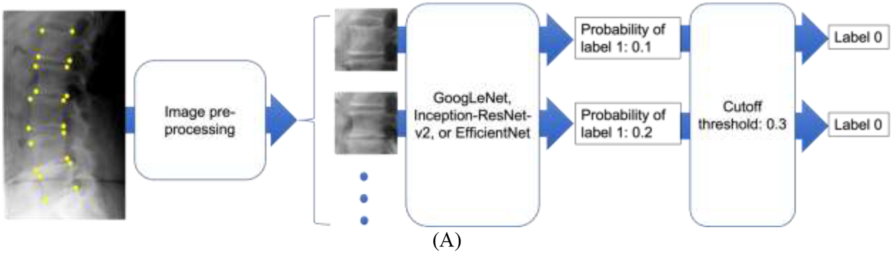
The flowchart of OCF classification using deep learning. Recall that the automatic image segmentation tool is a distinct body of work (see the INTRODUCTION section). In the current work, four manually annotated corner points of each vertebral body were used to extract the vertebral patch during image pre-processing. Taking an individual vertebral patch as an input, each of the five deep learning algorithms was used to build models to classify the vertebral patch to have label 0 or label 1. (A) shows the flowchart of OCF classification by GoogLeNet, Inception-ResNet-v2, or EfficientNet-B1. Each of these three models output a probability that the vertebral patch should be classified to have label 1. Then the vertebral patch was classified by comparing the probability and a pre-set cutoff threshold. (B) shows the flowchart of OCF classification by ensemble averaging, which averaged the probabilities output by the three individual models. Then the classification result was obtained by comparing the average probability and a pre-set cutoff threshold (details in the Model evaluation section of the MATERIALS AND METHODS section). (C) shows the flowchart of OCF classification by ensemble majority voting. The classification result of ensemble majority voting was the majority classification result of the three individual models.

After training the models using the three individual algorithms mentioned above, two ensemble models were created using the ensemble averaging algorithm and the ensemble majority voting algorithm (see Figures 3(B) and 3(C)).

In summary, three deep learning models and two ensemble models were generated in each of the following three training tasks :

1. Task 1: Pre-train the model on ImageNet and fine-tune the model on the MrOS-mSQ dataset’s training set (ImageNet → MrOS-mSQ).

2. Task 2: Pre-train the model on ImageNet and fine-tune the model on the local-m2ABQ dataset’s training set (ImageNet → local-m2ABQ).

3. Task 3: The model tuned in Task 1 was further fine-tuned on the local-m2ABQ dataset’s training set (ImageNet → MrOS-mSQ → local-m2ABQ).

In total, 15 models (5 models per task × 3 tasks) were built.

More details of model training are presented in Section B of the Supplemental Materials.

Model evaluation

Using both the local-m2ABQ dataset’s test set and the MrOS-m2ABQ dataset’s test set, we tested each of the 15 trained models described in the “Model training” section above. Each model trained in Task 1 was also tested on the MrOS-mSQ dataset’s test set. All of the performance measures mentioned in this section were computed using the classification results on individual vertebral patches.

The ensemble majority voting algorithm does not output a numerical value on which a range of cutoff thresholds can be set (see Figure 3(C)). Thus, the AUC-PR and the AUC-ROC of the models built using the ensemble majority voting algorithm could not be computed. Instead, the following performance measures were computed: accuracy, sensitivity, specificity, PPV, negative predictive value (NPV), false discovery rate (FDR=1–PPV), and F₁ score.

For the other trained models, all of the performance measures mentioned above were computed, including the AUC-PR and the AUC-ROC. For measures other than AUC-PR and AUC-ROC, a cutoff threshold was required. To set the cutoff threshold for each of these models, we used two thresholding methods, each applied to the validation set of the dataset whose training set was used to finally fine-tune the model. The same cutoff threshold was then used when testing the model on different test sets. The two thresholding methods are as follows:

1. Set the cutoff threshold to maximize the F₁ score. This automatically sets the cutoff threshold and balances the sensitivity and the PPV.

2. Manually set the threshold to make the PPV approximate 90%. Recall that we prioritize the PPV rather than the sensitivity for our opportunistic screening tool (see the INTRODUCTION section). Our initial consultation with local clinicians showed that a PPV of approximately 90% was appropriate.

The 95% confidence interval (CI) of each performance measure was computed using 2,000-fold bootstrap analysis.

IRB Approval

Retrieval of the local dataset was covered under the local retrospective institutional review board (IRB) for Diagnosis Radiology Images Deep Learning Project with a waiver of informed consent. For the MrOS dataset, at each medical center, a local IRB approved the MrOS study. All MrOS participants gave written informed consent at the time of the study.

RESULTS

Datasets

Table 2 shows the local dataset’s metadata, including age, sex, race, ethnicity, radiograph generation year, and X-ray system vendor. In Section D of the Supplemental Materials, we also show the number and the percentage of the local dataset’s radiographs generated by each type of machine. The MrOS dataset’s metadata have been summarized in multiple publications (35–37, 42) and are shown in Table 3. Section E of the Supplemental Materials shows more details of the metadata of the MrOS dataset’s training set.

Table 2.

Metadata for the training, validation, and test sets of the local dataset, as well as the entire local dataset. The age data were retrieved from the RIS. The sex data were obtained from the DICOM metadata of the radiographs. The race and ethnicity data were retrieved from the electronic health record system. A subject could have multiple exams, which might not be from the same year. Consequently, multiple ages could be recorded for a subject. In each set, for every range of ages, we reported the number of recorded ages rather than the number of subjects. If a subject had multiple ages recorded, all of them were used to calculate the mean and the standard deviation.

	Training set	Validation set	Test set	Entire local dataset
	Number (percentage) of recorded ages
Age at exam
65–74	395 (53.2%)	181 (59.0%)	479 (56.6%)	1,055 (55.7%)
75–84	234 (31.6%)	84 (27.4%)	255 (30.1%)	573 (30.2%)
85–94	98 (13.2%)	32 (10.4%)	102 (12.0%)	232 (12.2%)
≥95	15 (2.0%)	10 (3.2%)	11 (1.3%)	36 (1.9%)
	Number
Total recorded ages	742	307	847	1,896
	Mean ± standard deviation of ages in years
Female	76 ± 9	75 ± 9	75 ± 8	75 ± 8
Male	75 ± 9	75 ± 9	75 ± 9	75 ± 9
All	75 ± 9	75 ± 9	75 ± 9	75 ± 9
	Number (percentage) of subjects
Sex
Female	339 (53.3%)	172 (56.0%)	467 (55.1%)	978 (54.6%)
Male	296 (46.5%)	135 (44.0%)	379 (44.8%)	810 (45.3%)
Not recorded	1 (0.2%)	0 (0%)	1 (0.1%)	2 (0.1%)
Race
American Indian and Alaska Native	2 (0.3%)	2 (0.7%)	6 (0.7%)	10 (0.6%)
Asian	68 (10.7%)	37 (12.0%)	72 (8.5%)	177 (9.9%)
Black or African American	39 (6.2%)	20 (6.5%)	51 (6.0%)	110 (6.1%)
Native Hawaiian and Other Pacific Islander	2 (0.3%)	1 (0.3%)	3 (0.4%)	6 (0.3%)
White	474 (74.5%)	220 (71.7%)	654 (77.2%)	1348 (75.3%)
Multiple races	49 (7.7%)	25 (8.1%)	57 (6.7%)	131 (7.3%)
Not recorded	2 (0.3%)	2 (0.7%)	4 (0.5%)	8 (0.4%)
Ethnicity
Hispanic or Latino	9 (1.4%)	5 (1.6%)	16 (1.9%)	30 (1.7%)
Not Hispanic or Latino	189 (29.7%)	138 (45.0%)	358 (42.3%)	685 (38.3%)
Not recorded	438 (68.9%)	164 (53.4%)	473 (55.8%)	1,075 (60.0%)
	Number
Total subjects	636	307	847	1,790
	Number (percentage) of radiographs
Radiograph generation year
2000–2005	127 (17.1%)	49 (15.9%)	113 (13.3%)	289 (15.2%)
2006–2011	354 (47.7%)	135 (44.0%)	405 (47.8%)	894 (47.2%)
2012–2017	261 (35.2%)	123 (40.1%)	329 (38.9%)	713 (37.6%)
X-ray machine vendor
Canon	5 (0.7%)	0 (0%)	5 (0.6%)	10 (0.5%)
DeJarnette Research Systems	48 (6.5%)	21 (6.8%)	48 (5.7%)	117 (6.2%)
Fujifilm	378 (50.9%)	157 (51.2%)	427 (50.4%)	962 (50.8%)
General Electric	202 (27.2%)	74 (24.1%)	232 (27.3%)	508 (26.8%)
Philips	104 (14.0%)	50 (16.3%)	127 (15.0%)	281 (14.8%)
Hybrid General Electric and Fujifilm	5 (0.7%)	5 (1.6%)	8 (1.0%)	18 (0.9%)
	Number
Total radiographs	742	307	847	1,896

Table 3.

Demographic information for the subjects in each of the entire, training, validation, and test sets from the MrOS dataset. By listing in the “Sampled test set (m2ABQ)” column, we also show the demographic information of the subjects in the sampled test set with 122 radiographs annotated by the m2ABQ criteria (see the “MrOS dataset” section of the “MATERIALS AND METHODS” section). The mean ± standard deviation of the ages was recorded at the baseline (Visit 1) and the follow-up (Visit 2) visits. If a subject reported multi-races, each race would be recorded.

	Training set	Validation set	Entire test set	Sampled test set (m2ABQ)	Entire dataset
	Mean ± standard deviation
Age at Visit 1	73.7 ± 5.9	74.1 ± 6.2	73.5 ± 5.7	74.5 ± 5.8	73.7 ± 5.9
Age at Visit 2	77.8 ± 5.6	77.9 ± 5.6	77.5 ± 5.4	77.8 ± 5.3	77.7 ± 5.6
	Number (percentage) of subjects
Race/ethnicity
American Indian or Alaska Native	42 (0.8%)	7 (1.8%)	8 (1.2%)	0 (0.0%)	57 (0.9%)
Asian	159 (3.2%)	12 (3.1%)	25 (3.7%)	5 (4.8%)	196 (3.2%)
Black or African American	212 (4.2%)	21 (5.4%)	21 (3.1%)	4 (3.8)	254 (4.2%)
Hispanic or Latino	100 (2.0%)	11 (2.8%)	15 (2.2%)	0 (0.0%)	126 (2.1%)
Native Hawaiian or Other Pacific Islander	11 (0.2%)	3 (0.8%)	1 (0.1%)	1 (1.0%)	15 (0.2%)
White	4,492 (89.6%)	338 (86.1%)	611 (89.7%)	95 (90.4%)	5,441 (89.4%)

Model evaluation

We report the performance of our ensemble averaging algorithm in Tasks 2 (ImageNet → local-m2ABQ) and 3 (ImageNet → MrOS-mSQ → local-m2ABQ) in this manuscript and report the performance of the other models in Section C of the Supplemental Materials. The performance measures were computed using the classification results on individual vertebral patches.

Figures 4 and 5 show the performance of the model built using the ensemble averaging algorithm in Task 2. Figures 4 and 5 show this model’s performance on the local-m2ABQ dataset’s test set and the MrOS-m2ABQ dataset’s test set, respectively.

Figure 4.

The performance of the model, which was built using the ensemble averaging algorithm in Task 2 and evaluated on the test set of the local-m2ABQ dataset. (A) The ROC curve and the AUC-ROC with its 95% CI. (B) The PR curve and the AUC-PR with its 95% CI. (C) When the cutoff threshold (0.327) is set to maximize the F₁ score on the local-m2ABQ dataset’s validation set, the confusion matrix with the number of vertebral bodies in each of the four cells shown in the parentheses. (D) The confusion matrix when the cutoff threshold (0.800) is manually set to make the PPV approximate 90% on the local-m2ABQ dataset’s validation set. (E) Using each thresholding method, the sensitivity, specificity, PPV, NPV, FDR, F₁ score, and accuracy with their 95% CIs.

Figure 5.

The performance of the model, which was built using the ensemble averaging algorithm in Task 2 and evaluated on the test set of the MrOS-m2ABQ dataset. (A) The ROC curve and the AUC-ROC with its 95% CI. (B) The PR curve and the AUC-PR with its 95% CI. (C) When the cutoff threshold (0.327) is set to maximize the F₁ score on the local-m2ABQ dataset’s validation set, the confusion matrix with the number of vertebral bodies in each of the four cells shown in the parentheses. (D) The confusion matrix when the cutoff threshold (0.800) is manually set to make the PPV approximate 90% on the local-m2ABQ dataset’s validation set. (E) Using each thresholding method, the sensitivity, specificity, PPV, NPV, FDR, F₁ score, and accuracy with their 95% CIs.

On the local-m2ABQ dataset’s test set, the model mentioned above yielded an AUC-ROC of 0.948 and an AUC-PR of 0.730. After setting the cutoff threshold to make the PPV approximate 90% on the local-m2ABQ dataset’s validation set, this model achieved a sensitivity of 54.5%, a specificity of 99.7%, a PPV of 89.8%, an NPV of 97.9%, an FDR of 10.2%, an F₁ score of 0.671, and an accuracy of 97.7%.

On the MrOS-m2ABQ dataset’s test set, the model mentioned above yielded an AUC-ROC of 0.936 and an AUC-PR of 0.811. After setting the cutoff threshold to make the PPV approximate 90% on the local-m2ABQ dataset’s validation set, this model achieved a sensitivity of 47.8%, a specificity of 99.6%, a PPV of 94.8%, an NPV of 92.4%, an FDR of 5.2%, an F₁ score of 0.636, and an accuracy of 92.5%.

Figure 6 shows the performance of the model built using the ensemble averaging algorithm in Task 3 and evaluated on the local-m2ABQ dataset’s test set. This model yielded an AUC-ROC of 0.955 and an AUC-PR of 0.764. After setting the cutoff threshold to make the PPV approximate 90% on the local-m2ABQ dataset’s validation set, this model achieved a sensitivity of 53.9%, a specificity of 99.7%, a PPV of 89.4%, an NPV of 97.9%, an FDR of 10.6%, an F₁ score of 0.672, and an accuracy of 97.7%.

Figure 6.

The performance of the model, which was built using the ensemble averaging algorithm in Task 3 and evaluated on the test set of the local-m2ABQ dataset. (A) The ROC curve and the AUC-ROC with its 95% CI. (B) The PR curve and the AUC-PR with its 95% CI. (C) When the cutoff threshold (0.764) is set to maximize the F₁ score on the local-m2ABQ dataset’s validation set, the confusion matrix with the number of vertebral bodies in each of the four cells shown in the parentheses. (D) The confusion matrix when the cutoff threshold (0.900) is manually set to make the PPV approximate 90% on the local-m2ABQ dataset’s validation set. (E) Using each thresholding method, the sensitivity, specificity, PPV, NPV, FDR, F₁ score, and accuracy with their 95% CIs.

Comparison between the models

For each deep learning algorithm, there were three training tasks. Each model was tested using two or three test sets. Table 4 shows the F₁ score, the AUC-PR, and the AUC-ROC of each (deep learning algorithm, training task, test set) combination. In this section, each model’s cutoff threshold was set to maximize the F₁ score on the corresponding validation set.

Table 4.

F₁ scores, AUC-PR, and AUC-ROC for each (deep learning algorithm, training task, test set) combination. The AUC-PR and the AUC-ROC of the models built using the ensemble majority voting algorithm could not be computed (see the “Model evaluation” section of the “MATERIALS AND METHODS” section). In this table, yellow and magenta are used to mark the MrOS dataset and the local dataset, respectively.

Training task	Task 1: ImageNet → MrOS-mSQ			Task 2: ImageNet → local-m2ABQ		Task 3: ImageNet → MrOS-mSQ → local-m2ABQ
Test set	MrOS-mSQ	MrOS-m2ABQ	Local-m2ABQ	MrOS-m2ABQ	Local-m2ABQ	MrOS-m2ABQ	Local-m2ABQ
	F1 score
GoogLeNet	0.751	0.691	0.579	0.698	0.668	0.694	0.701
Inception-ResNet-V2	0.729	0.652	0.523	0.670	0.659	0.698	0.674
EfficientNet-B1	0.743	0.667	0.543	0.705	0.650	0.747	0.689
Ensemble averaging	0.773	0.677	0.566	0.729	0.684	0.761	0.702
Ensemble majority voting	0.776	0.648	0.553	0.706	0.694	0.713	0.712
	AUC-PR
GoogLeNet	0.817	0.782	0.606	0.784	0.698	0.804	0.736
Inception-ResNet-V2	0.798	0.795	0.636	0.809	0.656	0.801	0.696
EfficientNet-B1	0.816	0.796	0.628	0.785	0.703	0.808	0.746
Ensemble averaging	0.841	0.796	0.658	0.811	0.730	0.831	0.764
	AUC-ROC
GoogLeNet	0.990	0.897	0.918	0.927	0.941	0.933	0.949
Inception-ResNet-V2	0.993	0.925	0.914	0.930	0.925	0.922	0.947
EfficientNet-B1	0.993	0.914	0.916	0.914	0.941	0.933	0.958
Ensemble averaging	0.992	0.911	0.930	0.936	0.948	0.940	0.955

In the local dataset’s test set and the MrOS dataset’s test set, the percentages of vertebral bodies with label 1 are 4.5% (computed using the table at the bottom of Figure 2) and 1.1% (35), respectively. Because AUC-ROC is less suitable than AUC-PR for a highly imbalanced test set (48), the models are compared not using AUC-ROC but using the F₁ score and the AUC-PR.

DISCUSSION

The number of subjects in each of the training and test sets was determined by striking the balance between obtaining a large set and reducing manual annotation time. A large set is more likely to contain diverse data. Thus, a large training set can reduce model overfitting. A large test set can ensure accurate measures of model performance. However, since manual annotation is time-consuming, we could not wait to train and test our models after annotating a very large number of radiographs.

The ensemble averaging model trained in Task 2 achieved our pre-specified objectives of AUC-PR >0.70 and AUC-ROC >0.90 on both the local dataset and the MrOS dataset. When setting the cutoff threshold to make the PPV approximately 90% on the local-m2ABQ dataset’s validation set, we obtained high PPVs and specificities with moderate sensitivities on both datasets. This is acceptable for our clinical use case of an opportunistic screening tool described in the INTRODUCTION section, in which the PPV and specificity rather than the sensitivity should be prioritized. An opportunistic screening tool could be clinically useful with a moderate sensitivity and a high specificity or PPV. Given the volume of radiographic exams that cover some portion of the thoracic and lumbar spine at most medical institutions, it is prudent to consider the downstream effects of positive and negative predictive results. A positive predictive result would result in provider efforts guiding the patient to the appropriate clinical care as well as patient expense, worry, radiation exposure, and potential harm. A negative predictive result would result in no further action and would not affect the current standard of clinical care. Our opportunistic screening tool will only augment current clinical practice rather than replace radiologist interpretation or any other step in the current clinical workflow. In this setting, a false negative is a missed opportunity, but could still be possibly caught by the current standard of care. A false positive triggers extra work that has no obvious benefit to the patient but potential harm and financial burden. Our model with a PPV of about 90% and a sensitivity of about 50% can detect nearly half of the unreported fractured vertebral bodies with limited extra cost. It is worth noting that many diagnostic tests in use today have modest sensitivities. Papanicolaou smear has a sensitivity of 55.4% and a specificity of 94.6% (49).

In the “Comparison between the models” section of the RESULTS section, we compared the performance of each (deep learning algorithm, training task, test set) combination. We have six observations:

1. In each (training task, test set) combination, the models built using the two ensemble algorithms typically outperformed the other models.

2. In each (training task, test set) combination, the two ensemble algorithms typically produced models with similar F₁ scores. Unlike the ensemble majority voting algorithm that outputs categorical values, the ensemble averaging algorithm provided numerical outputs to which different cutoff thresholds could be applied. Thus, the ensemble averaging algorithm is more flexible and can be adapted for different clinical use cases.

3. In Task 2 (ImageNet → local-m2ABQ), the model built using the ensemble averaging algorithm had a better F₁ score and a higher AUC-PR on the MrOS-m2ABQ dataset than on the local-m2ABQ dataset. This shows that the model built using the ensemble averaging algorithm has some generalizability. Counterintuitively, this model performed worse on the test set of the local-m2ABQ dataset, whose training set was used for fine-tuning this model, than on the MrOS-m2ABQ dataset. The reason could be that the data in the local dataset are more diverse, especially in subject positioning and image artifacts, increasing difficulty of OCF classification.

4. On each test set, each model trained in Task 3 (ImageNet → MrOS-mSQ → local-m2ABQ) typically had a higher F₁ score and a better AUC-PR than the corresponding model trained in Task 2 (ImageNet → local-m2ABQ) did. Our transfer learning technique in Task 3 could improve models’ performance. However, since each model trained in Task 3 was tuned using both datasets, we cannot claim that this model is generalizable. We need more datasets to show these models’ generalizability.

5. In Task 1 (ImageNet → MrOS-mSQ), the AUC-PR of each model tested on the MrOS-mSQ dataset was higher than that of each model tested on the MrOS-m2ABQ dataset but to a limited degree (e.g., 5.7% for the ensemble averaging algorithm). This could imply that our two binary OCF labeling systems (simplified from the mSQ criteria and the m2ABQ criteria, respectively) are similar.

6. In Task 1, the F₁ score and the AUC-PR of each model tested on the MrOS-mSQ dataset were higher than those of each model tested on the local-m2ABQ dataset, respectively (e.g., 36.6% and 27.8% greater, respectively by the F1 score and the AUC-PR, for the ensemble averaging algorithm). The models fine-tuned on the MrOS-mSQ dataset were not generalizable to the local-m2ABQ dataset. The MrOS dataset was obtained for research, while the local dataset was extracted from clinical data that were more diverse in demographics, X-ray techniques, and image artifact variations. This greater diversity is likely the cause of poor performance by models only fine-tuned on the MrOS dataset.

Researchers from other research projects (25–29) reported approaches to automatically detecting OCFs using radiographs. Using lumbar or thoracolumbar spine radiographs, Chou et al. (25) did automatic segmentation to extract the vertebral bodies and classified each vertebral body using an ensemble method. Using similar methods, Li et al. (26) trained models to automatically detect vertebral fractures on lateral spine radiographs. Chen et al. (27) and Murata et al. (28) respectively trained a deep learning model to detect vertebral fractures on a radiograph without vertebral body segmentation. The main limitation of each of the above projects is that a single-site dataset was used. This resulted in a more homogeneous population, making the trained models less generalizable.

Xiao et al. (29) trained and tested their models on women’s lateral spine and chest radiographs from multiple sites, showing that their models had good generalizability and could serve as an opportunistic screening tool for female OCF screening. Based on their models, they developed a software program with a user interface. However, except for two datasets, they did not mention the source, the dataset construction process, and the demographic information of the other datasets in detail. The two known datasets were retrieved from the Osteoporotic fractures in women (MsOS) Hong Kong dataset (50). Like the MrOS dataset, the MsOS Hong Kong dataset was originally collected for research and has some selection bias. Their recruitment criteria included that all subjects were able to walk without assistance (50). The radiographs in this dataset likely contain far fewer imaging chain artifacts like angulation, position, overlapping, motion, and equipment, which are commonly seen in standard clinical imaging, and are seen when comparing the local and MrOS datasets in our study.

In contrast to the above projects, we used data assembled from multiple sites with detailed description of the dataset construction process and demographic information (see Figure 2 and Table 2 describing the local dataset, as well as the papers (35–37, 42) describing the MrOS dataset). Our local dataset was retrieved from local clinical sites and thus is more consistent with the distribution of clinical data. Shown in Table 2, the local dataset contains subjects that have varied race, ethnicity, and gender, as well as radiographs generated from different X-ray machines, which could help improve the generalizability of our trained models.

Our models have several limitations:

1. We used lateral spine radiographs to build our classifiers. This type of radiograph is optimized to show bones, and thus a rational initial target for research. However, to increase the target population in the future, other radiographs like lateral chest or abdominal radiographs should be used.

2. Our current model classifies individual vertebral bodies extracted from spine radiographs using manual annotation. This ensures that the vertebral bodies are correctly bounded on a radiograph but is not automated or scalable. As mentioned in the INTRODUCTION section, we are testing and separately reporting image segmentation models to automatically localize the vertebral bodies on a radiograph.

3. Currently, we only have one dataset (the local dataset) containing data acquired in varied clinical settings for diagnostic purposes. The number of annotated radiographs in the local dataset is small. We need more annotated clinical data to train our model and test its generalizability. In the future, we will annotate more radiographs from various clinical sites using semi-automated approaches.

4. In this study, the cutoff thresholds set using the two thresholding methods might not be the best for the clinical use case. We have already surveyed a variety of clinical providers to determine an acceptable performance threshold for automated opportunistic OCF screening. We will further analyze our survey results to determine the most appropriate cutoff threshold for the clinical use case.

5. In this study, we did not analyze incorrectly classified cases and explore how image features contribute to each model’s outputs. These two tasks should be implemented in the future to understand how the model works, its failure modes, and how to further improve the model.

In conclusion, we used five deep learning algorithms to train models that detected OCFs of vertebral bodies extracted from spine radiographs. The ensemble averaging model trained in Task 2 achieved our pre-specified objectives of AUC-PR >0.70 and AUC-ROC >0.90 on both the local dataset and the MrOS dataset. This model has good performance and some generalizability and can serve as a critical component of our future automated opportunistic screening tool.