Abstract
Background
Multiple sclerosis (MS) and neuromyelitis optica spectrum disorder (NMOSD) are the two mimic autoimmune diseases of the central nervous system, which are rare in East Asia. Quantitative detection of contrast-enhancing lesions (CELs) on contrast-enhancing T1-weighted magnetic resonance (MR) images is of great significance for assessing the disease activity of MS and NMOSD. However, it is challenging to develop automatic segmentation algorithms due to the lack of data. In this work, we present an automatic segmentation model of CELs based on Fully Convolutional with Attention DenseNet (FCA-DenseNet) and transfer learning strategy to address the challenge of CEL quantification in small-scale datasets.
Methods
A transfer learning approach was employed in this study, whereby pretraining was conducted using 77 MS subjects from the open access datasets (MICCAI 2016, MICCAI 2017, ISBI 2015) for white matter hyperintensity segmentation, followed by fine-tuning using 24 MS and NMOSD subjects from the local dataset for CEL segmentation. The proposed FCA-DenseNet combined the Fully Convolutional DenseNet and Convolutional Block Attention Module in order to improve the learning capability. A 2.5D data slicing strategy was used to process complex 3D MR images. U-Net, ResUNet, TransUNet, and Attention-UNet are used as comparison models to FCA-DenseNet. Dice similarity coefficient (DSC), positive predictive value (PPV), true positive rate (TPR), and volume difference (VD) are used as evaluation metrics to evaluate the performances of different models.
Results
FCA-DenseNet outperforms all other models in terms of all evaluation metrics, with a DSC of 0.661±0.187, PPV of 0.719±0.201, TPR of 0.680±0.254, and VD of 0.388±0.334. Transfer learning strategy has achieved success in building segmentation models on a small-scale local dataset where traditional deep learning approaches fail to train effectively.
Conclusions
The improved FCA-DenseNet, combined with transfer learning strategy and 2.5D data slicing strategy, has successfully addressed the challenges in constructing deep learning models on small-scale datasets, making it conducive to clinical quantification of brain CELs and diagnosis of MS and NMOSD.
Keywords: Transfer learning, neuromyelitis optica spectrum disorder (NMOSD), multiple sclerosis (MS), magnetic resonance imaging (MRI), segmentation
Introduction
Multiple sclerosis (MS) and neuromyelitis optica spectrum disorder (NMOSD) are the two mimic autoimmune diseases of the central nervous system (1). MS is the leading nontraumatic disabling disease in young adults (2), which often has the clinical features of dissemination in space (DIS) and/or dissemination in time (DIT) (3). While NMOSD remains a rare autoimmune inflammatory demyelinating disorder worldwide that is mediated by the water channel aquaporin-4 antibody (4), it has a higher prevalence in East Asians and the Blacks (5).
Magnetic resonance imaging (MRI) is the most widely used noninvasive technique for visualizing the lesions of neuroinflammatory diseases in vivo. Furthermore, the T2-weighted fluid-attenuated inversion recovery (T2-FLAIR) and contrast-enhancing T1-weighted (CE-T1W) imaging of the brain are crucial in reflecting the lesions, and therefore are the essential tools for the diagnosis and assessment of disease activity in MS and NMOSD (6,7).
Quantitative detection of white matter hyperintensity (WMH) lesions on T2-FLAIR images and the contrast-enhancing lesions (CELs) on T1W images [also referred to post gadolinium (Gd) T1W or post-Gd T1W images] are of great significance for routine clinical work in radiology departments and neuroscience studies. During follow-up, the new WMH of T2 image and the WMH enhancing by contrast medium is related to the activity of inflammation (8). Enhancement in new inflammatory demyelinating lesions is a short-lived feature (2–8 weeks, although typically <4 weeks) in most cases (9).
Deep learning has become the latest research direction for processing image data, and its algorithms are also employed in MRI analysis (10). In particular, deep learning has shown excellent performance in medical imaging segmentation (11). Furthermore, based on deep learning models, fully automatic WMH quantification methods are promising (12). Li et al. proposed ensembled 2D fully convolutional networks for WMH segmentation (13). The 2D models take 2D slices of 3D images as input, ignoring spatial information of 3D images and the relevance between 2D slices. Sundaresan et al. proposed a tri-planar U-Net for WMH segmentation (14). The tri-planar model takes 2D slices from three different planes, but the relevance between 2D slices is still ignored. Zhang et al. proposed a 2.5D data slicing strategy for processing 3D MRI data (15). By stacking 2D slices together, the 2.5D method effectively utilizes various characteristics of 3D Data.
However, compared with the disseminative WMH on T2-FLAIR images, the CELs on T1W images are sparser, more subtle, and often have ambiguous boundaries in MS and NMOSD patients (16). In recent years, only a few studies have used large-scale MS datasets for segmenting CELs. Coronado et al. proposed a 3D convolutional neural network (CNN) for segmenting CELs (17). The 3D model consumes significant computational resources during training and requires the use of large-scale datasets. The joint U-Net by Krishnan et al. for CELs segmentation (18) had applied the state-of-the-art 2.5D data slicing strategy to reduce the size of the model but still evaluated on a large-scale dataset.
In East Asia, the prevalence of MS is the lowest in the world (<5/100,000) (19). The CELs of NMOSD account for only 9–36% of the total brain, with a regional prevalence of 1.57/100,000 (20). The rarity of the diseases leads to a lack of data, making it difficult to perform CEL segmentation on small-scale local dataset using deep learning methods. Meanwhile, due to the lack of publicly available datasets with annotated CELs, it is a challenge for the development of CEL segmentation deep learning models on small-scale datasets.
The purpose of this study is to construct a deep learning-based MS/NMOSD CEL segmentation model. Considering the scarcity of MS and NMOSD CE-T1W images, we propose a transfer learning strategy based on the similarity between WMH and CEL. In addition, we use the 2.5D data slicing strategy to solve the problem that the 3D deep learning model is easy to overfit on small-scale data sets. We present this article in accordance with the TRIPOD reporting checklist (available at https://qims.amegroups.com/article/view/10.21037/qims-23-846/rc).
Methods
Datasets
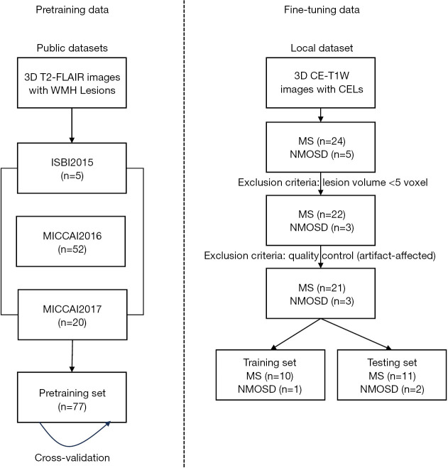
Two datasets were used in the experiments. The first dataset was used for pretraining, and it is an assemblage of three MS WMH segmentation public datasets: the ISBI 2015 MS Lesion Segmentation Challenge Dataset (ISBI 2015) (21), the MICCAI 2016 MS Lesion Segmentation Challenge Dataset (MICCAI 2016) (22) and the MICCAI 2017 MS Lesion Segmentation Challenge Dataset (MICCAI 2017) (23). The other local dataset is the CE-T1W lesion segmentation dataset retrospectively enrolled from a local hospital in China, which was used during the fine-tuning process. The study was conducted in accordance with the Declaration of Helsinki (as revised in 2013). This retrospective study was approved by the local ethics committee of the First Hospital of Jilin University. The informed written consent was provided by each participant prior to data collection and analysis. Figure 1 shows the usage of the two datasets.
Figure 1.
The composition of two datasets. T2-FLAIR, T2-weighted fluid-attenuated inversion recovery; WMH, white matter hyperintensity; CE-T1W, contrast-enhancing T1-weighted; CEL, contrast-enhancing lesion; MS, multiple sclerosis; NMOSD, neuromyelitis optica spectrum disorder.
The pretraining dataset
The first part of the pretraining dataset came from ISBI 2015, which was released by Carass et al. (21). It consisted of a training dataset of five MS patients with multiple time points. The 3D T2-FLAIR images in patients’ last time points were selected as part of the pretraining dataset in this study.
The second part of the pretraining dataset was from MICCAI 2016, which collected data from three centers following the same harmonic protocol (24). It contains 53 MS patients with MS. Fifty-two of them and their 3D T2-FLAIR magnetic resonance (MR) images were selected as the other part of the pretraining dataset in our study (one patient was excluded because the scan had no WMH lesions). All the 3D T2-FLAIR images were preprocessed using the nonlocal mean algorithm (25) and the N4 bias field correction algorithm (26).
The third part of the pretraining dataset was from MICCAI 2017, which also collected data from multiple different centers. The 3D T2-FLAIR data from its training set were used for the following experiments. A total of 20 images from 20 different MS patients was included in the third part.
Totally, 77 images (5 from ISBI 2015, 52 from MICCAI 2016, 20 from MICCAI 2017) from different subjects were included in the pretraining dataset to avoid the influence by longitudinal data.
The fine-tuning dataset
Local fine-tuning dataset including 24 MS and 5 NMOSD patients (8 males and 21 females; age 35±15 years; examination time 1/2019 to 9/2021) were retrospectively enrolled in our study. According to the inclusion criteria: images with at least one lesion of more than three voxels and without artifact, 21 MS and 3 NMOSD patients were retained. The NMOSD patients met the 2015 international consensus diagnostic criteria (4), and the MS patients were diagnosed fulfilled the recently revised diagnostic criteria (3,27). Table 1 presents the detailed information of the enrolled patients. All the subjects were examined using a 3.0 Tesla MR scanner (Ingenia, Philips Healthcare, the Netherlands), including the whole-brain CE-T1W sequences. Details of the MRI acquisition protocol are provided in appendix Table S1.
Table 1. Summary of clinical information and TLV of fine-tuning dataset.
| Metric | MS | NMOSD |
|---|---|---|
| No. of patients | 21 | 3 |
| Sex | ||
| Male | 7 | 0 |
| Female | 14 | 3 |
| Age (year) | ||
| Mean | 34.4±10.30 | 31±2.16 |
| Range | 16–52 | 28–33 |
| CEL-TLV (mL) | ||
| Mean | 0.320 | 0.930 |
| Median | 0.229 | 0.929 |
TLV was calculated based on manual lesion segmentation. TLV, total lesion volume; MS, multiple sclerosis; NMOSD, neuromyelitis optica spectrum disorder; CEL, contrast-enhancing lesion.
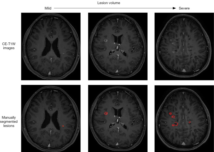
The CELs are defined as an area of at least 3 mm with a clear area of hyperintensity on T1-weighted images obtained at least 5 min after contrast agent administration. All the CELs were manually segmented using ITK-SNAP software (an open-source software package, www.itk-snap.org) (28) by a radiologist with more than eight years of diagnostic experience (L.A.) and validated by a senior neuroradiologist with more than 15 years of diagnostic experience (C.G.). The total lesion volume (TLV) in Table 1 is the quantification result of the manually segmented lesions. The brain-labeled CE-T1W images were selected as the local fine-tuning dataset. Figure 2 shows three subjects in the local dataset. From left to right are three different images with different lesion volume, which indicates the course of disease.
Figure 2.
Two MS CE-T1W images and one NMOSD CE-T1W image (the middle) in the local dataset. The images were manually segmented (colored sites represent the lesions). CE-T1W, contrast-enhancing T1-weighted; MS, multiple sclerosis; NMOSD, neuromyelitis optica spectrum disorder.
Data preprocessing and postprocessing
For the local dataset, Brain Extraction Tool (29) was used to extract brain tissue and remove the skull. After that, python toolkits NiBabel (30) and SimpleITK (31) were used to crop the field of view and resize the spacing of images to 1 mm × 1 mm × 1 mm. Kernel density estimation was used to normalize data and all images were randomly shifted and flipped with a 0.5 probability for augmentation. The lesion probability map predicted by the model was binarized by threshold with 0.5.
Transfer learning strategy
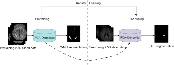
Transfer learning can be expressed as (32): giving a source data domain DS and a target data domain DT and their corresponding tasks TS and TT transfer the base model (TS) learned from the source data domain (DS) to a target model (TT) applied in the target domain (DT). The transfer strategy proposed in this paper uses the pretrained Fully Convolutional with Attention DenseNet (FCA-DenseNet) model as the base model on the pretraining dataset, then the pretrained model is fine-tuned to obtain the target model. Our transfer learning strategy can be summarized in two steps.
Firstly, during the pretraining process, a five-fold cross-validation training strategy was used on the pretraining dataset, in which all samples from the pretraining dataset were used as training data. The pretraining dataset was divided equally into five disjoint subsets. At the time of each training, one subset was selected as the testing set and the rest as the training set. After pretraining, five models were obtained as a result of the five-fold cross-validation strategy, and the model with the best performance was selected for fine-tuning.
Finally, the selected model continued to be trained on the local dataset. During the fine-tuning process, the model parameters saved from pretraining were used to initialize the model. The local dataset was randomly split into a training set and a testing set with a 1:1 ratio. The same transfer learning strategy was applied to all the selected pretrained comparation models. Figure 3 shows the transfer learning strategy.
Figure 3.
Transfer learning strategy. FCA-DenseNet, Fully Convolutional with Attention DenseNet; WMH, white matter hyperintensity; CEL, contrast-enhancing lesion.
FCA-DenseNet
In this paper, we propose a FCA-DenseNet as a base model for applying the transfer learning strategy. FCA-DenseNet uses Fully Convolutional DenseNet (FC-DenseNet) (33) as the backbone network, to which the Convolutional Block Attention Module (CBAM) is added. The network structure of FCA-DenseNet is shown in Figure 4.
Figure 4.
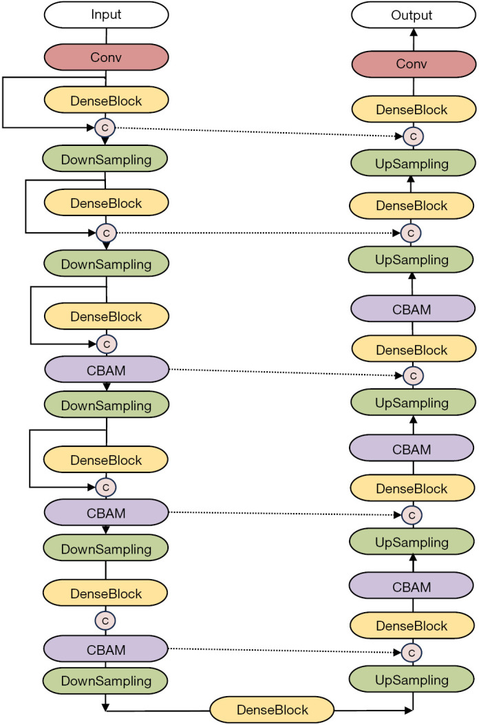
The network structure of FCA-DenseNet. Conv, convolution layer; C, concatenation; CBAM, Convolutional Block Attention Module; FCA-DenseNet, Fully Convolutional with Attention DenseNet.
FC-DenseNet backbone in FCA-DenseNet
FC-DenseNet, as the backbone network of FCA-DenseNet, was proposed by Jégou et al. in 2017 (33). FC-DenseNet is an improved U-Net structural model. It contains a downsampling path where the number of channels increases and the size of the feature map decreases and an upsampling path where the number of the channel becomes 1. At the end of the upsampling path, the model will output the probability distribution map of lesions which is the same size as the input.
FC-DenseNet combines the features of U-Net (34), ResNet (35), and DenseNet (36). It adds dense connections between convolutional layers in the network, and the input of each upsampling block is the concatenation of the output and input of its previous convolutional block.
CBAM in FCA-DenseNet
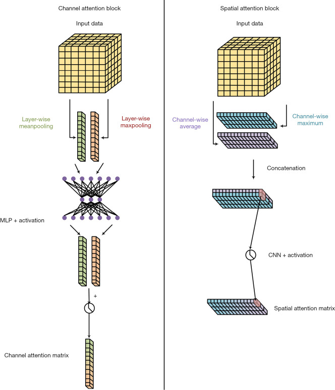
The CBAM was added to the FC-DenseNet. CBAM proposed by Woo et al. in 2018 comprises two types of attention computation: channel attention and spatial attention (37). Channel attention calculates the attention matrix at the channel level of the input data, giving higher weight to essential features and lower weight to irrelevant features. Spatial attention is calculated at a lower level, giving higher weight to important spatial parts of the data. Figure 5 shows the structure of CBAM.
Figure 5.
Structure of CBAM. MLP, multiple layer perceptron; CNN, convolutional neural network; CBAM, Convolutional Block Attention Module.
The channel attention first calculates the maximum and average pooling of the data in each channel, then concatenates the results of the different channels and outputs the channel attention matrix via a shared parameter multiple layer perceptron. The spatial attention first calculates the average and maximum value of each position of the data in different channels, merges the results of all positions, and then uses a CNN to output the spatial attention matrix.
Focal loss in FCA-DenseNet
Because of the small and sparse CELs on MR images, the problem of data imbalance affects the experiments. Therefore, our experiment used focal loss to reduce the error caused by sample imbalance (38). The focal loss is expressed as:
| [1] |
where p represents the probability that the model outputs, y represents the ground truth, α is the weighting factor used to balance positive and negative samples, and γ is the adjustment factor used to reduce the weight of easy-to-classify data so that the model pays more attention to difficult-to-classify data.
In the following experiments, gamma and alpha for models were set to 1 and 0.25 by default (15). Experiments were set to discuss the influence of different settings of focal loss on FCA-DenseNet.
2.5D MR image slicing strategy
In order to reduce the number of parameters of the 3D CNN model and avoid the loss of correlation information between 2D slices in the 2D CNN model, a 2.5D MR image data slicing strategy was used.
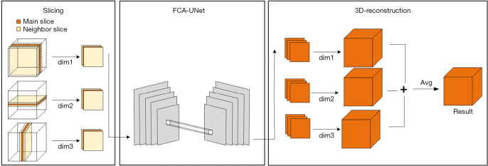
Firstly, the 3D MR image data were divided into 2.5D slices from three dimensions, each 2.5D slice containing a central main slice and multiple slices from its neighbor. The slices within each 2.5D slice were concatenated in the channel dimension, and the resulting multichannel data were used as the model input. For example, if using an image with a size of 256×128×64 as training data, assuming that each slice and its first pair of neighbors were merged into a 2.5D slice, the data would be divided into [256×(3, 128, 64)], [128×(256, 3, 64)], [64×(256, 128, 3)] from three dimensions. The number of neighbors of the main slice in the 2.5D slice is a hyperparameter; this was set at 3 by default; that is, for the i-th main slice, the i−1th and i+1th slices are merged into a 2.5D slice.
Secondly, during the training process, all 3D image data were divided into multiple 2.5D slices from three different dimensions, and these 2.5D slices were scrambled as 2.5D training data for model training. Model was trained with randomly shuffled batch of 2.5D slices. The model generated predictions for the central primary slice in the 2.5D slice, and a loss function was calculated between the prediction of each main slice and its corresponding ground truth label slice.
Finally, during the testing process, images were orderly sliced into 2.5D slices from three dimensions. For each individual dimension, 2.5D slices were sent into the model orderly for prediction. After the model output the prediction for all 2.5D slices in a single dimension, these ordered predictions were combined together to reconstruct the 3D lesion probability map with the corresponding order. From three dimensions, three 3D images were generated. These 3D images were added together by voxel and averaged to produce the model’s final prediction. Figure 6 shows the workflow of the 2.5D image slicing strategy.
Figure 6.
Workflow of the 2.5D image slicing strategy. FCA-DenseNet, Fully Convolutional with Attention DenseNet; dim, dimension; Avg, average.
In the following experiments, number of neighbors in 2.5D slices was set to 1-pair by default. And the shape of 2.5D slices was set to 256×256 by default. Experiments were set to discuss the influence of different number of neighbors in 2.5D slice on FCA-DenseNet.
Experiments
Experimental environment
In the experiment, four Nvidia RTX 2080Ti graphic cards, Intel Xeon 2.20 GHz CPU, 16 G memory, and the Ubuntu 22.04 operating system were used as the experimental environment. Pytorch (39) version 1.23.0 and CUDA version 11.3 were used as deep learning frameworks.
Hyperparameter settings
The images were randomly rotated and cropped during training. Images were randomly cropped into 256×256 image fragments, and, to avoid overfitting, only image fragments with lesions inside were retained as training data. The same hyperparameter settings were used for both pretraining and fine-tuning processes: three input channels, i.e., each main slice and its first pair of neighbors forming a 2.5D slice; the learning rate was set to 0.0002, and Adam optimizer with default parameters was used as the optimization algorithm (40). The batch size was set to 16, the maximum training epoch was set to 300, and there was an early stop strategy for 50 epochs.
Comparison experiments
To better evaluate the transfer strategy, multiple comparative experiments were conducted. First, to compare how the transfer strategy affected the different models, FC-DenseNet (33), U-Net (34), ResUNet (41), Attention-UNet (42), TransUNet (43), and FCA-DenseNet were all pretrained on the pretraining dataset, and the transfer strategy was applied to them for fine-tuning. Table 2 displays the specific information of each model, with TransUNet being a state-of-the-art method based on the transformer architecture.
Table 2. Implementation details of comparative models.
| Method | FCA-DenseNet | FC-DenseNet | U-Net | ResUNet | Attention-UNet | TransUNet |
|---|---|---|---|---|---|---|
| Parameters (M) | 1.4 | 1.3 | 2.0 | 3.2 | 2.1 | 105.3 |
| Training time (h) | ~10 | ~10 | ~7 | ~10 | ~7 | ~50 |
| Fine-tuning time (h) | ~5 | ~5 | ~3 | ~6 | ~3 | ~30 |
FCA-DenseNet, Fully Convolutional with Attention DenseNet; FC-DenseNet, Fully Convolutional DenseNet; M, million.
Second, to demonstrate the necessity and effectiveness of the transfer experiments, the models were directly trained and tested on the local dataset.
Finally, to verify whether the segmentation knowledge learned by the model from T2-FLAIR modality data can be directly applied to CE-T1W data, we directly used the pre-trained WMH segmentation model to test CE-T1W data.
Evaluation metrics
Multiple evaluation metrics were employed to assess the segmentation performance of each model, including Dice similarity coefficient (DSC), positive predictive value (PPV), true positive rate (TPR), and volume difference (VD).
| [2] |
where Υ represents the output of the model, represents the ground truth, represents the intersection operation of two matrices (if an element appears in both sets, it will be preserved in the result), and represents the number of elements in the matrix. The higher the DSC, the closer the prediction to the manually segmented label.
| [3] |
where true positive (TP) represents the number of positive voxels in both the label and the prediction result and false positive (FP) indicates the number of negative voxels predicted to be positive. A higher PPV indicates that the impact from the noise caused by them on the model is smaller.
| [4] |
where false negative (FN) indicates the number of positive voxels predicted to be negative. The higher the TPR, the stronger the model’s ability to identify lesions.
| [5] |
where TPp represents the number of predicted TP voxels and TPg represents the number of lesion voxels in the ground truth. VD is used to evaluate the accuracy of model segmentation from the perspective of the ground truth lesion volume. A lower VD indicates a better agreement between the predicted and true lesion volumes.
In addition to these metrics, for the CEL segmentation task, lesion false discovery rate (LFDR) and lesion sensitivity (L-sensitivity) were also utilized as supplementary evaluation criteria.
The lesions with a total volume of less than three voxels were excluded during the evaluation process (44). Specifically, for the remaining lesions, we considered them as TP if the predicted result had a sufficient overlap with the ground truth lesion. Conversely, if there was no overlap between the predicted result and the ground truth lesion, we regarded it as a FN case, indicating that the model failed to detect the lesion.
| [6] |
| [7] |
Results
Pretraining experimental results
All models were pretrained on the pretraining dataset using the same 2.5D slicing strategy. FC-DenseNet and FCA-DenseNet were set to 5×4 configuration, i.e., there were five dense blocks during up-sampling and down-sampling, each containing four dense layers. The average DSC, PPV, TPR, and VD in the cross-validation results of these models are shown in Table 3.
Table 3. Quantitative performances of different models on testing set of pretraining datasets.
| Method | FCA-DenseNet | FC-DenseNet | U-Net | ResUNet | Attention-UNet | TransUNet |
|---|---|---|---|---|---|---|
| DSC | 0.719 (0.014) | 0.714 (0.024) | 0.734 (0.009*) | 0.725 (0.013) | 0.736 (0.009) | 0.749* (0.088*) |
| PPV | 0.708 (0.039) | 0.698 (0.062) | 0.746* (0.021) | 0.662 (0.047) | 0.681 (0.040) | 0.709 (0.088) |
| TPR | 0.780 (0.041) | 0.785 (0.035) | 0.765 (0.029) | 0.841* (0.045*) | 0.830 (0.041) | 0.810 (0.079) |
| VD | 0.502 (0.305) | 0.527 (0.281) | 0.312 (0.080*) | 0.524 (0.136) | 0.398 (0.197) | 0.243* (0.182*) |
Data are presented as mean (standard deviation). *, the best performance. FCA-DenseNet, Fully Convolutional with Attention DenseNet; FC-DenseNet, Fully Convolutional DenseNet; DSC, Dice similarity coefficient; PPV, positive predictive value; TPR, true positive rate; VD, volume difference.
TransUNet achieved the best performance on the pretraining dataset, with a DSC of 0.749, although its PPV and TPR were not optimal. On the other hand, FCA-DenseNet performed comparatively worse, with a DSC of only 0.719. It is important to note that pretraining experiments were not the main focus of this study. However, it is worth mentioning that TransUNet, with a larger number of parameters, demonstrated state-of-the-art results on a stable large-scale publicly available dataset.
Additionally, all the pretrained models were tested on the local dataset. Table 4 presents the quantitative results of these pretrained models on the local dataset.
Table 4. Performances of different pretrained models on testing set of the local dataset.
| Method | FCA-DenseNet | FC-DenseNet | U-Net | ResUNet | Attention-UNet | TransUNet |
|---|---|---|---|---|---|---|
| DSC | 0.384 (0.303) | 0.224 (0.167) | 0.188 (0.183) | 0.343 (0.265) | 0.419 (0.252) | 0.157 (0.157) |
| PPV | 0.415 (0.307) | 0.156 (0.133) | 0.261 (0.248) | 0.363 (0.299) | 0.665 (0.292) | 0.238 (0.279) |
| TPR | 0.444 (0.348) | 0.156 (0.314) | 0.248 (0.232) | 0.413 (0.282) | 0.400 (0.304) | 0.329 (0.287) |
| VD | 10.654 (28.261) | 6.675 (14.226) | 2.602 (6.804) | 2.008 (3.227) | 0.644 (0.615) | 44.99 (135.216) |
| LFDR | 0.801 (0.202) | 0.852 (0.266) | 0.863 (0.176) | 0.784 (0.095) | 0.367 (0.216) | 0.786 (0.258) |
| L-sensitivity | 0.542 (0.341) | 0.661 (0.317) | 0.562 (0.342) | 0.588 (0.282) | 0.582 (0.333) | 0.628 (0.326) |
Data are presented as mean (standard deviation). FCA-DenseNet, Fully Convolutional with Attention DenseNet; FC-DenseNet, Fully Convolutional DenseNet; DSC, Dice similarity coefficient; PPV, positive predictive value; TPR, true positive rate; VD, volume difference; LFDR, lesion false discovery rate; L-sensitivity, lesion sensitivity.
All the pretrained models for WMH segmentation performed poorly in CEL segmentation, with DSC scores below 0.5. Furthermore, except for Attention-UNet, all models exhibited significantly higher VD, indicating that WMH shares a higher similarity with the hyperintensity regions in CE-T1W images, whereas CEL possesses more unique characteristics.
Directly training experimental results
All models were directly trained on the local dataset to test their segmentation ability on small-scale datasets. Table 5 presents the results of these experiments. When using the same hyperparameter settings as fine-tuning experiments and pretraining experiments, directly training of all models cannot obtain effective results, as the output is blank and the DSC is 0. To further explore the reason of such result, the input size was changed to 64×64. As can be seen in Table 5, the small input size relatively reduces the imbalance of the data, but also limited the performance of models. Besides, transformer-based TransUNet cannot handle training with 64×64 and testing with 256×256, for the self-attention structure is different from CNNs.
Table 5. The performance of different models trained directly on testing set of the local dataset.
| Method | FCA-DenseNet | FC-DenseNet | U-Net | ResUNet | Attention-UNet | TransUNet |
|---|---|---|---|---|---|---|
| DSC | 0.559 (0.238) | 0.560 (0.206) | 0.503 (0.264) | 0.537 (0.256) | 0.604 (0.235) | NA/0 |
| PPV | 0.567 (0.230) | 0.570 (0.223) | 0.507 (0.288) | 0.561 (0.296) | 0.624 (0.266) | NA/0 |
| TPR | 0.657 (0.265) | 0.669 (0.246) | 0.575 (0.316) | 0.592 (0.299) | 0.631 (0.275) | NA/0 |
| VD | 0.913 (1.554) | 0.894 (1.279) | 0.644 (0.602) | 0.616 (0.653) | 0.428 (0.400) | NA/1 |
| LFDR | 0.753 (0.182) | 0.781 (0.149) | 0.787 (0.133) | 0.775 (0.130) | 0.771 (0.147) | NA/1 |
| L-sensitivity | 0.720 (0.286) | 0.784 (0.253) | 0.672 (0.316) | 0.723 (0.297) | 0.701 (0.316) | NA/0 |
Data are presented as mean (standard deviation). FCA-DenseNet, Fully Convolutional with Attention DenseNet; FC-DenseNet, Fully Convolutional DenseNet; DSC, Dice similarity coefficient; PPV, positive predictive value; TPR, true positive rate; VD, volume difference; LFDR, lesion false discovery rate; L-sensitivity, lesion sensitivity.
Fine-tuning experimental results
All the pretrained models applied to transfer learning strategy on the local dataset. Table 6 shows the results of testing on the local dataset after fine-tuning.
Table 6. Fine-tuning experimental results of different methods on testing set of local dataset.
| Method | FCA-DenseNet | FC-DenseNet | U-Net | ResUNet | Attention-UNet | TransUNet |
|---|---|---|---|---|---|---|
| DSC | 0.661* (0.187)* | 0.611 (0.227) | 0.525 (0.278) | 0.545 (0.217) | 0.589 (0.240) | 0.502 (0.191) |
| PPV | 0.719* (0.201)* | 0.669 (0.216) | 0.570 (0.305) | 0.527 (0.238) | 0.687 (0.254) | 0.560 (0.270) |
| TPR | 0.680* (0.254)* | 0.667 (0.280) | 0.538 (0.322) | 0.644 (0.253) | 0.619 (0.286) | 0.538 (0.256) |
| VD | 0.388* (0.334)* | 0.460 (0.448) | 0.461 (0.314) | 0.707 (1.350) | 0.641 (0.910) | 0.565 (0.332) |
| LFDR | 0.416* (0.295)* | 0.519 (0.229) | 0.427 (0.273) | 0.644 (0.157) | 0.478 (0.235) | 0.457 (0.339) |
| L-sensitivity | 0.768* (0.230)* | 0.730 (0.289) | 0.641 (0.368) | 0.764 (0.230) | 0.699 (0.271) | 0.701 (0.319) |
Data are presented as mean (standard deviation). *, the best performance. FCA-DenseNet, Fully Convolutional with Attention DenseNet; FC-DenseNet, Fully Convolutional DenseNet; DSC, Dice similarity coefficient; PPV, positive predictive value; TPR, true positive rate; VD, volume difference; LFDR, lesion false discovery rate; L-sensitivity, lesion sensitivity.
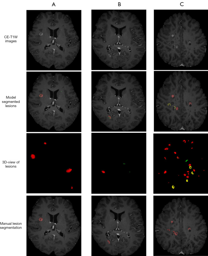
FCA-DenseNet achieved the best model performance among all metrics. In particular, the TPR performance is much greater than other models, which means that the attention module can improve the model’s ability to identify lesion voxels. Figure 7 shows the FCA-DenseNet prediction for CELs after fine-tuning.
Figure 7.
MS (B and C) and NMOSD (A) segmentation results from the FCA-DenseNet after fine-tuning. The colored parts represent different results, red for TP, green for FP, and yellow for FN. CE-T1W, contrast-enhancing T1-weighted; MS, multiple sclerosis; FCA-DenseNet, Fully Convolutional with Attention DenseNet; TP, true positive; FP, false positive; FN, false negative.
Ablation experimental results
Ablation experiments of various loss functions
To demonstrate the effectiveness of focal loss, we conducted comparative fine-tuning experiments, contrasting it with cross-entropy (CE) and Dice loss (45) while keeping other parameter settings the same. Table 7 displays the training results for different loss functions, while Figure 8 illustrates the training curve specifically for the utilization of focal loss.
Table 7. Experimental results of FCA-DenseNet after fine-tuning with different loss functions on testing set of local dataset.
| Loss | Focal | CE | Dice |
|---|---|---|---|
| DSC | 0.661* (0.187)* | 0.642 (0.181) | 0.639 (0.221) |
| PPV | 0.719 (0.201) | 0.778* (0.197)* | 0.758 (0.235) |
| TPR | 0.680* (0.254)* | 0.615 (0.243) | 0.611 (0.267) |
| VD | 0.388* (0.334)* | 0.430 (0.275) | 0.423 (0.291) |
| LFDR | 0.416 (0.295) | 0.340 (0.275) | 0.315* (0.308)* |
| L-sensitivity | 0.768* (0.230)* | 0.702 (0.306) | 0.737 (0.286) |
Data are presented as mean (standard deviation). *, the best performance. FCA-DenseNet, Fully Convolutional with Attention DenseNet; DSC, Dice similarity coefficient; CE, cross-entropy; PPV, positive predictive value; TPR, true positive rate; VD, volume difference; LFDR, lesion false discovery rate; L-sensitivity, lesion sensitivity.
Figure 8.
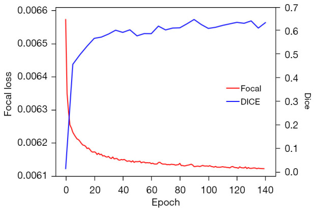
Training curves utilizing focal loss.
The focal loss achieved the highest DSC compared to the CE and Dice loss functions. It allows the model to a greater focus on the segmentation of small lesions, despite the increase in FP and the decrease in PPV. Overall, the segmentation performance has improved.
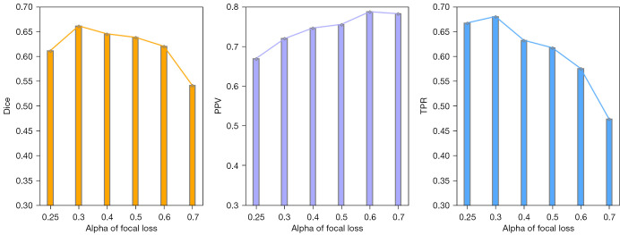
To validate the effectiveness of the focal loss, experiments were conducted on focal losses with different hyperparameter settings. Figure 9 presents the training results using different alpha settings for focal loss.
Figure 9.
Influence of FCA-DenseNet in fine-tuning process with different alpha settings in focal loss. FCA-DenseNet, Fully Convolutional with Attention DenseNet; PPV, positive predictive value; TPR, true positive rate.
The parameter alpha in focal loss determines the importance of minority samples in imbalanced datasets. As alpha increases, the model gradually focuses more on minority lesion voxels. Experimental results indicate that the variation of alpha has a significant impact on the focal loss. When alpha is excessively large, the model becomes overly attentive to lesions, resulting in a higher number of FN and a lower number of FP, leading to changes in PPV and TPR.
Ablation experiments of 2.5D data slicing strategy
In order to further investigate the impact of the 2.5D data slicing strategy on the experiments, ablation experiments were conducted by varying the number of neighboring slices.
Table 8 indicates that the model achieves the best performance when incorporating one pair of neighboring slices for each slice. Too many or too few neighboring slices can result in a decrease in performance. In particular, when the number of input neighbors is excessive, the model may struggle to converge due to the imbalance in the data and the presence of irrelevant information, leading to ineffective experimental results.
Table 8. Experimental results of FCA-DenseNet after fine-tuning with different number of neighbors in 2.5D slice on testing set of local dataset.
| 2.5D strategy | 0 neighbor (2D) | 1 neighbor | 2 neighbors | 3 neighbors |
|---|---|---|---|---|
| DSC | 0.563 (0.251) | 0.661* (0.187)* | 0.618 (0.184) | NA |
| PPV | 0.658 (0.277) | 0.719* (0.201)* | 0.635 (0.229) | NA |
| TPR | 0.556 (0.301) | 0.680* (0.254)* | 0.696 (0.240) | NA |
| VD | 0.714 (0.345) | 0.388* (0.334)* | 0.576 (0.615) | NA |
| LFDR | 0.419 (0.243) | 0.416* (0.295)* | 0.575 (0.247) | NA |
| L-sensitivity | 0.649 (0.294) | 0.768 (0.230) | 0.775* (0.250)* | NA |
Data are presented as mean (standard deviation). *, the best performance. FCA-DenseNet, Fully Convolutional with Attention DenseNet; 2D, 2-dimensional; DSC, Dice similarity coefficient; PPV, positive predictive value; TPR, true positive rate; VD, volume difference; LFDR, lesion false discovery rate; L-sensitivity, lesion sensitivity; NA, not applicable.
Discussion
Pretraining experiments
The pretraining experiments involved the fusion of MR images from multiple WMH segmentation datasets. Given the variations in imaging parameters and preprocessing methods across different data sources, the models’ generalization capability is of high importance. The average DSC of all models reached 0.729±0.012, indicating a relatively stable performance across the publicly available datasets, although there are performance differences among different models. TransUNet, benefiting from the latest self-attention method and a large number of parameters, exhibits strong learning capability and segmentation performance on large-scale datasets compared to CNN models with fewer parameters. On the other hand, FCA-DenseNet demonstrates average performance on the pretraining dataset that involves multi-source data fusion. However, it is still able to successfully complete the WMH segmentation task. The results in Table 4 show that, because of the difference between the T2-FLAIR and CE-T1W data, the model obtained from WMH segmentation could not output proper results for CEL segmentation. A few of the CELs can be segmented by the models trained for WMH segmentation, which has confirmed that there was indeed a relative similarity between WMH and enhancing lesions.
It is generally acknowledged that training deep learning models on small-scale datasets can be challenging, and our experiments further confirm this limitation. By training the models directly on the local dataset, as evident from Table 5, all models still output invalid results, although we have employed various data augmentation strategies. This observation highlights the challenges of applying deep learning to real clinical data.
Fine-tuning experiments and ablation experiments
The pretraining and fine-tuning method in transfer learning has proven to be highly effective for modeling on small-scale datasets. After applying transfer learning strategies, all models exhibited significant performance improvements in the CEL segmentation task.
According to Table 6, FCA-DenseNet achieved the best performance in CEL segmentation with a DSC of 0.661, PPV of 0.719, TPR of 0.668, VD of 0.388, LFDR of 0.416, and L-sensitivity of 0.768. This indicates that FCA-DenseNet effectively learned the distinguishing characteristics of both CEL lesions and other brain tissues. On the other hand, the backbone model FC-DenseNet performed poorly, suggesting that the addition of attention mechanisms made the model more efficient in learning image features within the same domain. In contrast, U-Net, ResUNet, and Attention-UNet, which exhibited better generalization performance in pretraining, performed poorly on the specific CEL segmentation data. Surprisingly, TransUNet, which performed best on the pretraining dataset, performed worst in the CEL segmentation task. This suggests that the self-attention architecture with a large number of parameters may not be the most suitable choice for certain specific medical image processing tasks.
Deep learning methods generally strive for improved performance by augmenting training data and adopting a 2:1 or 4:1 ratio for training and testing set split. This approach serves to mitigate the deleterious impact of individual sample noise on the model. Despite the difficulties in obtaining CE-T1W data and training with a relatively small-scale dataset, we chose an unusual 1:1 training set split.
Multiple ablation experiments further validate the effectiveness of the proposed method. Focal loss, compared to CE and Dice loss, significantly improves the training performance of the models. Moreover, by adjusting the parameters of focal loss, the model’s learning ability on different samples can be controlled. Table 7, Figure 8, and Figure 9 provide evidence for the importance of the choice of loss function. The 2.5D image slicing strategy serves as the foundation and core data processing method in our experiments. We conducted experiments to determine the optimal number of neighboring slices to be merged. As shown in Table 8, the best results are achieved when incorporating the information from one neighboring slice, indicating that merging too much neighboring information may cause the model to learn irrelevant image features, while using too few neighboring slices may lead to insufficient feature learning.
In conclusion, the success in FCA-DenseNet can be quote in two points: first, the transfer learning strategy brings efficient training. Second the CBAM blocks propagate features through spatial and channel, on such an imbalanced dataset, helping the model absorb more information from the entire input space.
Medical significance and limitations
We only used CE-T1W data for the segmentation of CELs in the experiment, and the performance did not significantly decrease compared to the commonly used multi-modality approach, which has stronger guiding significance for clinical diagnosis. Despite the rarity of the disease, our method can still successfully segment small and discrete CELs, even with a small-scale training dataset. It has great significance for clinical assisted diagnosis of MS and NMOSD.
This experiment also has certain limitations. The scarcity of clinical real-world data has resulted in a limited training dataset, which has impacted the experimental results to some extent. It needs to be emphasized again that MS and NMOSD are two rare diseases in East Asia, make it very difficult to collect clinical data. In the future, with the acquisition of more data, the model can be further optimized to improve the differentiation of blood vessels and other tissues that are similar to CEL. Additionally, due to the rarity of MS and NMOSD and the specific characteristics of CELs, the performance of the model on datasets with varying distributions of CEL lesions needs to be evaluated.
Conclusions
In this paper, we propose a novel 2.5D FCA-DenseNet network with a transfer learning strategy for the segmentation of CELs on CE-T1W MR images of MS and NMOSD. The proposed transfer learning strategy can effectively resolve the problems caused by scarce data and sparse lesions. In addition, the 2.5D image slicing strategy reduces the overall complexity of the model, enhances the training data, expands the data features, and results in better segmentation performance.
Although many deep-learning MR image segmentation methods have been proposed in recent years, they cannot obtain suitable segmentation of the MR image in cases of small-scale experimental data. This deficiency can make it difficult for models to assist in the diagnosis of rare diseases, such as MS and NMOSD. The scarcity and complexity of CE-T1W MR images of MS and NMOSD pose challenges for further research. Also, the bias caused by different MR scanners/centers and the similarity between CELs and blood vessels in CE-T1W MR images are still the problems in the present. Improvement of deep learning algorithms and transfer strategies for accurate segmentation of CELs remain the direction and focus of our future work.
Supplementary
The article’s supplementary files as
Acknowledgments
Funding: This work was supported by the National Natural Science Foundation of China (No. 62072212), the Development Project of Jilin Province of China (Nos. 20220508125RC, 20230201065GX), the Jilin Provincial Key Laboratory of Big Data Intelligent Cognition (No. 20210504003GH), the Natural Science Foundation of Jilin Province (No. 20210101273JC), and the Science and Technology Achievement Transformation Fund of the First Hospital of Jilin University (No. JDYY2021-A0010).
Ethical Statement: The authors are accountable for all aspects of the work in ensuring that questions related to the accuracy or integrity of any part of the work are appropriately investigated and resolved. The study was conducted in accordance with the Declaration of Helsinki (as revised in 2013). This retrospective study was approved by the local ethics committee of the First Hospital of Jilin University. The informed written consent was provided by each participant prior to data collection and analysis.
Footnotes
Reporting Checklist: The authors have completed the TRIPOD reporting checklist. Available at https://qims.amegroups.com/article/view/10.21037/qims-23-846/rc
Conflicts of Interest: All authors have completed the ICMJE uniform disclosure form (available at https://qims.amegroups.com/article/view/10.21037/qims-23-846/coif). G.H. is the employee of Philips Healthcare, Beijing, China. The other authors have no conflicts of interest to declare.
References
- 1.Matthews L, Marasco R, Jenkinson M, Küker W, Luppe S, Leite MI, Giorgio A, De Stefano N, Robertson N, Johansen-Berg H, Evangelou N, Palace J. Distinction of seropositive NMO spectrum disorder and MS brain lesion distribution. Neurology 2013;80:1330-7. 10.1212/WNL.0b013e3182887957 [DOI] [PMC free article] [PubMed] [Google Scholar]
- 2.Dobson R, Giovannoni G. Multiple sclerosis - a review. Eur J Neurol 2019;26:27-40. 10.1111/ene.13819 [DOI] [PubMed] [Google Scholar]
- 3.Thompson AJ, Banwell BL, Barkhof F, Carroll WM, Coetzee T, Comi G, et al. Diagnosis of multiple sclerosis: 2017 revisions of the McDonald criteria. Lancet Neurol 2018;17:162-73. 10.1016/S1474-4422(17)30470-2 [DOI] [PubMed] [Google Scholar]
- 4.Wingerchuk DM, Banwell B, Bennett JL, Cabre P, Carroll W, Chitnis T, de Seze J, Fujihara K, Greenberg B, Jacob A, Jarius S, Lana-Peixoto M, Levy M, Simon JH, Tenembaum S, Traboulsee AL, Waters P, Wellik KE, Weinshenker BG, International Panel for NMO Diagnosis . International consensus diagnostic criteria for neuromyelitis optica spectrum disorders. Neurology 2015;85:177-89. 10.1212/WNL.0000000000001729 [DOI] [PMC free article] [PubMed] [Google Scholar]
- 5.Liu C, Shi M, Zhu M, Chu F, Jin T, Zhu J. Comparisons of clinical phenotype, radiological and laboratory features, and therapy of neuromyelitis optica spectrum disorder by regions: update and challenges. Autoimmun Rev 2022;21:102921. 10.1016/j.autrev.2021.102921 [DOI] [PubMed] [Google Scholar]
- 6.Wattjes MP, Ciccarelli O, Reich DS, Banwell B, de Stefano N, Enzinger C, et al. 2021 MAGNIMS-CMSC-NAIMS consensus recommendations on the use of MRI in patients with multiple sclerosis. Lancet Neurol 2021;20:653-70. 10.1016/S1474-4422(21)00095-8 [DOI] [PubMed] [Google Scholar]
- 7.Kim HJ, Paul F, Lana-Peixoto MA, Tenembaum S, Asgari N, Palace J, Klawiter EC, Sato DK, de Seze J, Wuerfel J, Banwell BL, Villoslada P, Saiz A, Fujihara K, Kim SH; Guthy-Jackson Charitable Foundation NMO International Clinical Consortium & Biorepository. MRI characteristics of neuromyelitis optica spectrum disorder: an international update. Neurology 2015;84:1165-73. 10.1212/WNL.0000000000001367 [DOI] [PMC free article] [PubMed] [Google Scholar]
- 8.Wang B, Li X, Li H, Xiao L, Zhou Z, Chen K, Gui L, Hou X, Fan R, Chen K, Wu W, Li H, Hu X. Clinical, Radiological and Pathological Characteristics Between Cerebral Small Vessel Disease and Multiple Sclerosis: A Review. Front Neurol 2022;13:841521. 10.3389/fneur.2022.841521 [DOI] [PMC free article] [PubMed] [Google Scholar]
- 9.Filippi M, Preziosa P, Banwell BL, Barkhof F, Ciccarelli O, De Stefano N, Geurts JJG, Paul F, Reich DS, Toosy AT, Traboulsee A, Wattjes MP, Yousry TA, Gass A, Lubetzki C, Weinshenker BG, Rocca MA. Assessment of lesions on magnetic resonance imaging in multiple sclerosis: practical guidelines. Brain 2019;142:1858-75. 10.1093/brain/awz144 [DOI] [PMC free article] [PubMed] [Google Scholar]
- 10.Lundervold AS, Lundervold A. An overview of deep learning in medical imaging focusing on MRI. Z Med Phys 2019;29:102-27. 10.1016/j.zemedi.2018.11.002 [DOI] [PubMed] [Google Scholar]
- 11.Maier A, Syben C, Lasser T, Riess C. A gentle introduction to deep learning in medical image processing. Z Med Phys 2019;29:86-101. 10.1016/j.zemedi.2018.12.003 [DOI] [PubMed] [Google Scholar]
- 12.Balakrishnan R, Valdés Hernández MDC, Farrall AJ. Automatic segmentation of white matter hyperintensities from brain magnetic resonance images in the era of deep learning and big data - A systematic review. Comput Med Imaging Graph 2021;88:101867. 10.1016/j.compmedimag.2021.101867 [DOI] [PubMed] [Google Scholar]
- 13.Li H, Jiang G, Zhang J, Wang R, Wang Z, Zheng WS, Menze B. Fully convolutional network ensembles for white matter hyperintensities segmentation in MR images. Neuroimage 2018;183:650-65. 10.1016/j.neuroimage.2018.07.005 [DOI] [PubMed] [Google Scholar]
- 14.Sundaresan V, Zamboni G, Rothwell PM, Jenkinson M, Griffanti L. Triplanar ensemble U-Net model for white matter hyperintensities segmentation on MR images. Med Image Anal 2021;73:102184. 10.1016/j.media.2021.102184 [DOI] [PMC free article] [PubMed] [Google Scholar]
- 15.Zhang H, Valcarcel AM, Bakshi R, Chu R, Bagnato F, Shinohara RT, Hett K, Oguz I. Multiple Sclerosis Lesion Segmentation with Tiramisu and 2.5D Stacked Slices. Med Image Comput Comput Assist Interv 2019;11766:338-46. [DOI] [PMC free article] [PubMed] [Google Scholar]
- 16.Chan KH, Tse CT, Chung CP, Lee RL, Kwan JS, Ho PW, Ho JW. Brain involvement in neuromyelitis optica spectrum disorders. Arch Neurol 2011;68:1432-9. 10.1001/archneurol.2011.249 [DOI] [PubMed] [Google Scholar]
- 17.Coronado I, Gabr RE, Narayana PA. Deep learning segmentation of gadolinium-enhancing lesions in multiple sclerosis. Mult Scler 2021;27:519-27. 10.1177/1352458520921364 [DOI] [PMC free article] [PubMed] [Google Scholar]
- 18.Krishnan AP, Song Z, Clayton D, Gaetano L, Jia X, de Crespigny A, Bengtsson T, Carano RAD. Joint MRI T1 Unenhancing and Contrast-enhancing Multiple Sclerosis Lesion Segmentation with Deep Learning in OPERA Trials. Radiology 2022;302:662-73. 10.1148/radiol.211528 [DOI] [PubMed] [Google Scholar]
- 19.Koch-Henriksen N, Sørensen PS. The changing demographic pattern of multiple sclerosis epidemiology. Lancet Neurol 2010;9:520-32. 10.1016/S1474-4422(10)70064-8 [DOI] [PubMed] [Google Scholar]
- 20.Tian DC, Li Z, Yuan M, Zhang C, Gu H, Wang Y, Shi FD. Incidence of neuromyelitis optica spectrum disorder (NMOSD) in China: A national population-based study. Lancet Reg Health West Pac 2020;2:100021. 10.1016/j.lanwpc.2020.100021 [DOI] [PMC free article] [PubMed] [Google Scholar]
- 21.Carass A, Roy S, Jog A, Cuzzocreo JL, Magrath E, Gherman A, et al. Longitudinal multiple sclerosis lesion segmentation: Resource and challenge. Neuroimage 2017;148:77-102. 10.1016/j.neuroimage.2016.12.064 [DOI] [PMC free article] [PubMed] [Google Scholar]
- 22.Commowick O, Kain M, Casey R, Ameli R, Ferré JC, Kerbrat A, Tourdias T, Cervenansky F, Camarasu-Pop S, Glatard T, Vukusic S, Edan G, Barillot C, Dojat M, Cotton F. Multiple sclerosis lesions segmentation from multiple experts: The MICCAI 2016 challenge dataset. Neuroimage 2021;244:118589. 10.1016/j.neuroimage.2021.118589 [DOI] [PubMed] [Google Scholar]
- 23.Kuijf HJ, Biesbroek JM, De Bresser J, Heinen R, Andermatt S, Bento M, et al. Standardized Assessment of Automatic Segmentation of White Matter Hyperintensities and Results of the WMH Segmentation Challenge. IEEE Trans Med Imaging 2019;38:2556-68. 10.1109/TMI.2019.2905770 [DOI] [PMC free article] [PubMed] [Google Scholar]
- 24.Brisset JC, Kremer S, Hannoun S, Bonneville F, Durand-Dubief F, Tourdias T, Barillot C, Guttmann C, Vukusic S, Dousset V, Cotton F; Collaborators. New OFSEP recommendations for MRI assessment of multiple sclerosis patients: Special consideration for gadolinium deposition and frequent acquisitions. J Neuroradiol 2020;47:250-8. 10.1016/j.neurad.2020.01.083 [DOI] [PubMed] [Google Scholar]
- 25.Coupe P, Yger P, Prima S, Hellier P, Kervrann C, Barillot C. An optimized blockwise nonlocal means denoising filter for 3-D magnetic resonance images. IEEE Trans Med Imaging 2008;27:425-41. 10.1109/TMI.2007.906087 [DOI] [PMC free article] [PubMed] [Google Scholar]
- 26.Tustison NJ, Avants BB, Cook PA, Zheng Y, Egan A, Yushkevich PA, Gee JC. N4ITK: improved N3 bias correction. IEEE Trans Med Imaging 2010;29:1310-20. 10.1109/TMI.2010.2046908 [DOI] [PMC free article] [PubMed] [Google Scholar]
- 27.Polman CH, Reingold SC, Banwell B, Clanet M, Cohen JA, Filippi M, Fujihara K, Havrdova E, Hutchinson M, Kappos L, Lublin FD, Montalban X, O'Connor P, Sandberg-Wollheim M, Thompson AJ, Waubant E, Weinshenker B, Wolinsky JS. Diagnostic criteria for multiple sclerosis: 2010 revisions to the McDonald criteria. Ann Neurol 2011;69:292-302. 10.1002/ana.22366 [DOI] [PMC free article] [PubMed] [Google Scholar]
- 28.Yushkevich PA, Piven J, Hazlett HC, Smith RG, Ho S, Gee JC, Gerig G. User-guided 3D active contour segmentation of anatomical structures: significantly improved efficiency and reliability. Neuroimage 2006;31:1116-28. 10.1016/j.neuroimage.2006.01.015 [DOI] [PubMed] [Google Scholar]
- 29.Smith SM. Fast robust automated brain extraction. Hum Brain Mapp 2002;17:143-55. 10.1002/hbm.10062 [DOI] [PMC free article] [PubMed] [Google Scholar]
- 30.Brett M, Markiewicz CJ, Hanke M, Côté MA, Cipollini B, McCarthy P, Cheng CP, Halchenko YO, Cottaar M, Ghosh S, et al. Nipy/Nibabel: 3.0.0. Zenodo; Geneve, Switzerland; 2019.
- 31.Lowekamp BC, Chen DT, Ibáñez L, Blezek D. The Design of SimpleITK. Front Neuroinform 2013;7:45. 10.3389/fninf.2013.00045 [DOI] [PMC free article] [PubMed] [Google Scholar]
- 32.Zhuang F, Qi Z, Duan K, Xi D, Zhu Y, Zhu H, Xiong H, He Q, et al. A comprehensive survey on transfer learning. Proceedings of the IEEE 2020;109:43-76. [Google Scholar]
- 33.Jégou S, Drozdzal M, Vazquez D, Romero A, Bengio Y, editors. The one hundred layers tiramisu: Fully convolutional DenseNets for semantic segmentation. Proceedings of the IEEE Conference on Computer Vision and Pattern Recognition Workshops; Honolulu, HI, USA; 2017. [Google Scholar]
- 34.Ronneberger O, Fischer P, Brox T. U-Net: Convolutional Networks for Biomedical Image Segmentation. In: Navab N, Hornegger J, Wells W, Frangi A, editors. Medical Image Computing and Computer-Assisted Intervention – MICCAI 2015. MICCAI 2015. Lecture Notes in Computer Science, Springer, Cham; 2015;9351. [Google Scholar]
- 35.He K, Zhang X, Ren S, Sun J, editors. Deep residual learning for image recognition. Proceedings of the IEEE Conference on Computer Vision and Pattern Recognition; Las Vegas, NV, USA; 2016. [Google Scholar]
- 36.Huang G, Liu Z, van der Maaten L, Weinberger KQ, editors. Densely connected convolutional networks. Proceedings of the IEEE Conference on Computer Vision and Pattern Recognition; Honolulu; 2017:4700-8. [Google Scholar]
- 37.Woo S, Park J, Lee JY, Kweon IS, editors. CBAM: Convolutional block attention module. Proceedings of the European Conference on Computer Vision (ECCV); Xiamen, China; 2018:3-19. [Google Scholar]
- 38.Lin TY, Goyal P, Girshick R, He K, Dollar P. Focal Loss for Dense Object Detection. IEEE Trans Pattern Anal Mach Intell 2020;42:318-27. 10.1109/TPAMI.2018.2858826 [DOI] [PubMed] [Google Scholar]
- 39.Paszke A, Gross S, Massa F, Lerer A, Bradbury J, Chanan G, Killeen T, Lin Z, Gimelshein N, Antiga L, Desmaison A, Kopf A, Yang E, DeVito Z, Raison M, Tejani A, Chilamkurthy S, Steiner B, Fang L, Bai J, Chintala S. Pytorch: An imperative style, high-performance deep learning library. Advances in Neural Information Processing Systems. 2019;32. [Google Scholar]
- 40.Kingma DP, Ba J. Adam: A method for stochastic optimization. arXiv preprint. arXiv 2014. doi: 10.48550/arxiv.1412.6980. [DOI]
- 41.Diakogiannis FI, Waldner F, Caccetta P, Wu C. ResUNet-a: A deep learning framework for semantic segmentation of remotely sensed data. ISPRS Journal of Photogrammetry and Remote Sensing. 2020;162:94-114. [Google Scholar]
- 42.Oktay O, Schlemper J, Folgoc LL, Lee M, Heinrich M, Misawa K, Mori K, McDonagh S, Hammerla NY, Kainz B, Glocker B, Rueckert D. Attention u-net: Learning where to look for the pancreas. arXiv preprint. arXiv 2018. doi: 10.48550/arXiv.1804.03999. [DOI]
- 43.Chen J, Lu Y, Yu Q, Luo X, Adeli E, Wang Y, Lu L, Yuille AL, Zhou Y. Transunet: Transformers make strong encoders for medical image segmentation. arXiv preprint. arXiv 2021. doi: 10.48550/arXiv.2102.04306. [DOI]
- 44.Cacciaguerra L, Meani A, Mesaros S, Radaelli M, Palace J, Dujmovic-Basuroski I, Pagani E, Martinelli V, Matthews L, Drulovic J, Leite MI, Comi G, Filippi M, Rocca MA. Brain and cord imaging features in neuromyelitis optica spectrum disorders. Ann Neurol 2019;85:371-84. 10.1002/ana.25411 [DOI] [PubMed] [Google Scholar]
- 45.Milletari F, Navab N, Ahmadi SA, editors. V-net: Fully convolutional neural networks for volumetric medical image segmentation. 2016 Fourth International Conference on 3D Vision (3DV); Stanford, CA, USA; 2016: IEEE. [Google Scholar]
Associated Data
This section collects any data citations, data availability statements, or supplementary materials included in this article.
Supplementary Materials
The article’s supplementary files as


