Cluster Gauss‐Newton method for a quick approximation of profile likelihood: With application to physiologically‐based pharmacokinetic models

Abstract

Physiologically‐based pharmacokinetic (PBPK) models can be challenging to work with because they can have too many parameters to identify from observable data. The profile likelihood method can help solve this issue by determining parameter identifiability and confidence intervals, but it involves repetitive parameter optimizations that can be time‐consuming. The Cluster Gauss‐Newton method (CGNM) is a parameter estimation method that efficiently searches through a wide range of parameter space. In this study, we propose a method that approximates the profile likelihood by reusing intermediate computation results from CGNM, allowing us to obtain the upper bounds of the profile likelihood without conducting additional model evaluation. This method allows us to quickly draw approximate profile likelihoods for all unknown parameters. Additionally, the same approach can be used to draw two‐dimensional profile likelihoods for all parameter combinations within seconds. We demonstrate the effectiveness of this method on three PBPK models.

Study Highlights.

• WHAT IS THE CURRENT KNOWLEDGE ON THE TOPIC?

Profile likelihood can be used to determine parameter identifiability and confidence interval of the physiologically‐based pharmacokinetic (PBPK) model; however, it is a computationally intensive process.

• WHAT QUESTION DID THIS STUDY ADDRESS?

Is it possible to obtain profile likelihood quickly and easily?

• WHAT DOES THIS STUDY ADD TO OUR KNOWLEDGE?

Profile likelihood can be approximated by reusing the intermediate computation results of the parameter estimation via the Cluster Gauss‐Newton method (CGNM), hence, it can be drawn quickly without additional model evaluation and can be done easily with R‐package CGNM.

• HOW MIGHT THIS CHANGE DRUG DISCOVERY, DEVELOPMENT, AND/OR THERAPEUTICS?

Use of profile likelihood analyses may become a standard procedure of PBPK model‐based analysis in pharmacokinetics.

INTRODUCTION

Background

Given the complexity of physiology and the limitation of experimentally observable quantities, physiologically‐based mechanistic (PBPK) models often become overparameterized mathematical models. That is to say, the unknown model parameter combination cannot be uniquely estimated from the observed data. The Cluster Gauss‐Newton method (CGNM) is an algorithm inspired by this overparameterized nature of the physiologically‐based mechanistic models (e.g., PBPK models), and it finds multiple best‐fit parameter combinations of a fixed‐effect model. ¹ CGNM and its predecessor the Cluster Newton method ² have been used previously by several authors ³ , ⁴ , ⁵ , ⁶ , ⁷ , ⁸ , ⁹ to analyze PBPK models and a systems pharmacology model.

The CGNM can be used to estimate the model parameters that are themselves of pharmacological interest. For example, Mochizuki et al. ¹⁰ and Yoshikado et al. ¹¹ have shown that human in vivo inhibition constants (K _i value) for the organic anion transporter (OATP1Bs) can be estimated from the endogenous biomarker even if the PBPK model used to analyze the data is overparameterized, hence, not all parameters can be estimated uniquely. Despite these conclusions being visually trivial when presented as the plot of parameter distribution, it is desirable to have a statistically rigorous criterion for parameter identifiability. One way to establish parameter‐wise identifiability is to use profile likelihood. ¹²

In addition, the confidence interval of identifiable parameters can be derived using profile likelihood. ¹³ Roughly speaking, profile likelihood is a surface of maximum likelihood with various fixed parameters. Each point drawn as the profile likelihood requires each parameter estimation to find the maximum likelihood; hence, it can be a computationally intensive process. In this paper, we propose a method to quickly approximate the profile likelihood by reusing the computation done during CGNM parameter estimation; hence, without extra parameter estimation nor model evaluation.

Cluster Gauss‐Newton method

Mathematically speaking, the CGNM is an algorithm to numerically approximate solutions of nonlinear‐least squares problems. In other words, a method that minimizes the sum of squares residual (SSR) where minimizing SSR is equivalent to maximizing likelihood assuming symmetric distributions of the residual.

The CGNM method can be considered as a multi‐start method where the algorithm starts from multiple initial estimates and obtains multiple approximate minimizers of the nonlinear‐least squares problem. Then, the minima of these approximate minimizers are accepted as the multiple best‐fit parameter combinations.

As the readers probably have experienced, minimizers or SSR (equivalently parameter combinations that maximize likelihood) found by the computational algorithm can depend on the initial estimate, and the multi‐start method is intended to remedy this issue as well as to identify nonidentifiable parameters by obtaining multiple parameter combinations that minimize the SSR. Instead of naively repeating the conventional optimization methods with multiple initial estimates, we have developed a mathematical algorithm CGNM to increase the computation efficiency for the multi‐start method. In this paper, we have initially introduced CGNM, ¹ and we have shown the CGNM is a computationally efficient and robust algorithm by comparing it with nine conventional and state‐of‐the‐art algorithms.

Simply speaking, CGNM conducts Gauss‐Newton‐type iterations from various initial iterates. The initial iterates are generated randomly within the user‐specified initial range. The key idea of CGNM is that instead of using a Jacobian matrix that is approximated or calculated for each initial iterate, CGNM approximates a Jacobian‐like matrix collectively using all initial iterates. This has been shown to give a significant advantage in computation speed and robustness. The collectively approximated Jacobian is used to update the initial iterate and repeat this process until a desired convergence criterion is met. Because of the nature of this approach, CGNM evaluates a wide range of parameter combinations that minimize SSR within and near the user‐specified initial range. The proposed method for approximating profile likelihood makes use of this nature of the CGNM.

Once the multiple best‐fit parameter combinations are found, one can conduct further simulations using these multiple parameter combinations. In this way, the user can discuss and draw a conclusion about the simulation study while considering multiple possible simulation results that originate from the fact that some parameters are not identifiable. For example, recently, Lee et al. ¹⁴ have shown that the despite that not all model parameters can be identified from the data, the time‐course profile of receptor occupancy of warfarin can be simulated uniquely when plasma concentration with clear target‐mediated drug disposition (TMDD) is observable. The conventional approach to this type of problem was to simplify the model structure or fix the model parameters so that all the unfixed model parameters become identifiable and conduct main analyses, then conduct post hoc sensitivity analyses by repeating the analyses with various fixed parameters to confirm the main finding is not influenced by the assumed fixed parameter. The CGNM‐based analyses can avoid this lengthy process and directly discuss the main conclusion taking the unidentifiable nature of the model into account.

The CGNM can easily be implemented following pseudo code available in ref. [1]; however, actively maintained R implementations is currently available on CRAN. ¹⁵ In this paper, we show that in addition to fast and robust parameter estimation of the overparameterized model using CGNM, the profile likelihood can be obtained at almost no additional computation cost (i.e., no further parameter estimation nor a model evaluation).

METHODS

The key idea of the proposed methodology is to make use of the wide range of model evaluations done during the CGNM iterations and draw profile likelihood. CGNM starts iterations from a range of initial iterates that the user specified as the range of interest (e.g., range of physiologically or kinetically plausible parameters) and algorithmically searches through this range to find minimizers. Thus, by combining all the model evaluations that were done during the iterations gives a wide range of model evaluations to draw profile likelihood. In addition, because this collection of model evaluations is done algorithmically, one can see that there are more model evaluations in the parameter space where SSRs are smaller. In other words, the profile likelihood drawn based on this collection of CGNM model evaluations will have better resolution near where SSR is smaller and rougher resolution in the parameter space where SSR is larger. Roughly speaking, we draw profile likelihood by first binning the parameter combinations by the quantile of the parameter that we are drawing the profile likelihood for and then finding the minimum SSR (hence the maximum likelihood) among these already evaluated parameter combinations within the bin. Then the approximation of the profile likelihood can be drawn using these parameter values and corresponding SSRs. Note that we denote this as “approximate” profile likelihood because we are not conducting optimization with fixed parameter values at each point where we draw the likelihood surface. Hence, strictly speaking, what we draw using the proposed method is an upper bound of the profile likelihood. If one requires a more accurate profile likelihood, the approximate profile likelihood can be used as the initial estimate and conduct further optimization.

The mathematical formulation of the approximate profile likelihood

The key concept of the profile likelihood is to divide the parameters into a low dimensional parameter of interest and a high dimensional nuisance parameter. ¹⁶ Then obtain the maximum likelihood given parameter in the parameter of interest, that is:

$$\mathrm{pl}\left(\mathbf{\theta }\right)=\underset{\mathbf{\eta }}{\sup }l\left(\mathbf{\theta },\mathbf{\eta }\right)$$

where $\mathrm{pl}$ is the profile likelihood which is a function of $\mathbf{\theta }$, and $l$ is the full likelihood which is a function of both $\mathbf{\theta }$ and $\mathbf{\eta }$. The vector $\mathbf{\theta }$ is the parameters of interest, $\mathbf{\eta }$ is the vector of nuisance parameters. Note, in this paper, we represent a vector quantity with bold‐faced font and a scalar quantity with a normal font. In addition, we limit our interest for the case where we are interested in either one or two dimensions of the parameter of interest so that we can visually represent the profile likelihood. For simplicity of representation, we for now focus our discussion on the case of one‐dimension profile, that is to say:

$$\begin{array}{r}\mathrm{p}{\mathrm{l}}_m\left(\theta \right)=\underset{\mathbf{x}\in \left(\mathbf{x}|x_m=\theta \right)}{\sup }l\left(\mathbf{x}\right)\end{array}$$

where $\mathrm{p}{\mathrm{l}}_m$ is the profile likelihood of the $m\mathrm{th}$ parameter dimension, $\theta$ is a scalar value (note here it is not bold‐face font so it is a scaler quantity as we are only considering one‐dimensional profile likelihood) of the $m\mathrm{th}$ parameter, $\mathbf{x}$ is the parameter vector (including both parameter of interest and nuisance parameter, i.e., $\mathbf{x}=\left(\mathbf{\theta },\mathbf{\eta }\right)$), $x_m$ is the $m\mathrm{th}$ element of the parameter vector $\mathbf{x}$.

As can be clearly deduced from the above mathematical notation, the profile likelihood is a scalar function of a single variable. In our context, we treat these functions as being piecewise continuous near the maximum likelihood. To graphically represent a piecewise continuous function, we evaluate it at a finite set of points. Often, these points are connected by line segments to approximate the function using continuous piecewise linear functions. Let us denote these points as $\left\{a_1,a_2,\dots ,a_N\right\}$, where we aim to estimate the profile likelihood function for visualization purposes. For ease in notation, we label these points by their indices in ascending order, thus ensuring $a_{j-1}<a_j$. Essentially, plotting the profile likelihood involves solving a series of optimization problems to obtain points in x–y plane $\left(a_j,\mathrm{p}{\mathrm{l}}_m\left(a_j\right)\right)$ where

$$\begin{array}{r}\mathrm{p}{\mathrm{l}}_m\left(a_j\right)=\underset{\mathbf{x}\in \left(\mathbf{x}|x_m=a_j\right)}{\sup }l\left(\mathbf{x}\right)\text{for}j=1,2,\dots ,N.\end{array}$$

It is crucial to note that performing these optimizations at the fixed points $\left\{a_1,a_2,\dots ,a_N\right\}$ can be time‐consuming and computationally intensive. Moreover, because these optimizations are executed numerically, their precision hinges on the appropriateness of the chosen algorithm to the specific model or problem at hand.

The primary goal of our proposed methodology is to enhance computational efficiency by bypassing this exhaustive series of optimization tasks. The key idea of proposed methodology is to approximate ${\sup }_{\mathbf{x}\in \left(\mathbf{x}|x_m=a_j\right)}l\left(\mathbf{x}\right)$ by already computed likelihood during the CGNM iteration, that is:

$$\begin{array}{r}\mathrm{p}{\mathrm{l}}_m\left(a_j\right)\gtrsim l\left({\mathbf{x}}_j^{*}\right)\end{array}$$

where

$$\begin{array}{r}{\mathbf{x}}_j^{*}={\text{argmax}}_{\mathbf{x}\in \left\{{\mathbf{x}}^1,{\mathbf{x}}^2,{\mathbf{x}}^3,\dots \left|\frac{a_{j-1}+a_j}{2}<x_m<\frac{a_j+a_{j+1}}{2}\right.\right\}}l\left(\mathbf{x}\right)\end{array}$$

Here, ${\mathbf{x}}^1,{\mathbf{x}}^2,{\mathbf{x}}^3,\dots$ are the parameter combinations (represented as vectors) whose model evaluations were conducted during CGNM iteration hence likelihoods for these parameter combinations are available without additional model evaluation. We finally draw a point on the approximate profile likelihood plot $\left(x_{m,j}^{*},l\left({\mathbf{x}}_j^{*}\right)\right)$ where $x_{m,j}^{*}$ is the $m\mathrm{th}$ element of the vector ${\mathbf{x}}_j^{*}$, and the first element in $\left(·,·\right)$ represents the position on x‐axis and the second element represents the position on y‐axis.

One can easily imagine that $\left(x_{m,j}^{*},l\left({\mathbf{x}}_j^{*}\right)\right)$ approaches to the true profile likelihood as $\left\{{\mathbf{x}}^1,{\mathbf{x}}^2,{\mathbf{x}}^3,\dots \right\}$ become more dense sampling.

The same concept can be applied and implemented to the case of two‐dimensional parameter of interest. We approximate the two‐dimensional profile likelihood of $m\mathrm{th}\text{and}n\mathrm{th}$ parameters at the finite number of points $\left\{\left(a_j,b_k\right)\right\}$ and here we let $a_{j-1}<a_j$, $b_{k-1}<b_k$ and

$$\begin{array}{r}\mathrm{p}{\mathrm{l}}_{\mathit{mn}}\left(a_j,b_k\right)\gtrsim l\left({\mathbf{x}}_{\mathit{jk}}^{*}\right)\end{array}$$

where

$$\begin{array}{r}{\mathbf{x}}_{\mathit{jk}}^{*}={\text{argmax}}_{\mathbf{x}\in \left\{{\mathbf{x}}^1,{\mathbf{x}}^2,{\mathbf{x}}^3,\dots \left|\frac{a_{j-1}+a_j}{2}<x_m<\frac{a_j+a_{j+1}}{2}\text{and}\frac{b_{k-1}+b_k}{2}<x_n<\frac{b_k+b_{k+1}}{2}\right.\right\}}l\left(\mathbf{x}\right)\end{array}.$$

Then, we can draw a point on the approximate profile likelihood surface plot $\left(x_{m,\mathit{jk}}^{*},x_{n,\mathit{jk}}^{*},l\left({\mathbf{x}}_{\mathit{jk}}^{*}\right)\right)$ where $x_{m,\mathit{jk}}^{*}$ is the $m\mathrm{th}$ element of the vector ${\mathbf{x}}_{\mathit{jk}}^{*}$, $x_{n,\mathit{jk}}^{*}$ is the $n\mathrm{th}$ element of the vector ${\mathbf{x}}_{\mathit{jk}}^{*}$, and the first element in $\left(·,·,·\right)$ represents the position on x‐axis, the second element represents the position on y‐axis, and the third element represents the position on z‐axis.

Pseudo code for the algorithm to draw approximate profile likelihood using CGNM computation result

1. Let CGNM solve the following nonlinear least squares problem:

   $$\begin{array}{r}{\text{argmin}}_{\mathbf{x}}\parallel \mathbf{f}\left(\mathbf{x}\right)-{\mathbf{y}}^{*}{\parallel }_2\end{array}$$

   where $\mathbf{f}$ is the mathematical model (function from the model parameter combination to model simulation), $\mathbf{x}$ is a vector of the model parameter combination, and ${\mathbf{y}}^{*}$ is a vector of the observation.
   During CGNM iteration, algorithm computes the matrices $X^{\left(k\right)}$ and $Y^{\left(k\right)}$ where each row of $X^{\left(k\right)}$ contains a vector of parameter combination, each row of $Y^{\left(k\right)}$ contains a vector of model simulation, that is:

   $$\begin{array}{r}{\mathbf{y}}_i^{\left(k\right)}=\mathbf{f}\left({\mathbf{x}}_i^{\left(k\right)}\right)\text{for}i=1,2,\dots ,n\end{array}$$

   where ${\mathbf{x}}_i^{\left(k\right)}$ and ${\mathbf{y}}_i^{\left(k\right)}$ are $i\mathrm{th}$ rows of matrices $X^{\left(k\right)}$ and $Y^{\left(k\right)}$, respectively, $n$ is the number of parameter combinations in each iterate, and $\left(k\right)$ is the iteration number. The core idea of CGNM is to approximate Jacobian matrices efficiently from matrices $X^{\left(k\right)}$ and $Y^{\left(k\right)}$.
2. Combine all matrices $X^{\left(k\right)}$ into one matrix

   $$\begin{array}{r}X=\left[\begin{array}{c}{X}^{\left(0\right)}\\ X^{\left(1\right)}\\ ⋮\\ X^{\left(k\right)}\end{array}\right]\end{array}$$

   similar to matrices $Y^{\left(k\right)}$

   $$\begin{array}{r}Y=\left[\begin{array}{c}{Y}^{\left(0\right)}\\ Y^{\left(1\right)}\\ ⋮\\ Y^{\left(k\right)}\end{array}\right]\end{array}$$
3. Remove duplicated row of matrix $X$ from both matrix $X$ and $Y$, e.g., if ${\mathbf{x}}_i={\mathbf{x}}_j$ then update $X$ and $Y$ to

   $$\begin{array}{r}\left[\begin{array}{c}⋮\\ {\mathbf{x}}_i\\ ⋮\\ {\mathbf{x}}_{j-1}\\ {\mathbf{x}}_{j+1}\\ ⋮\end{array}\right]\text{and}\left[\begin{array}{c}⋮\\ {\mathbf{y}}_i\\ ⋮\\ {\mathbf{y}}_{j-1}\\ {\mathbf{y}}_{j+1}\\ ⋮\end{array}\right].\end{array}$$
4. calculate SSRs from matrix $Y$ and store them in a vector $\mathbf{r}$ that is:

   $$\begin{array}{r}{r}_i=\parallel {\mathbf{y}}_i-{\mathbf{y}}^{*}{\parallel }_2^2\end{array}$$

   where $r_i$ is the $i\mathrm{th}$ element of vector $\mathbf{r}$.
5. We now convert SSRs to likelihood

   $$\begin{array}{r}{l}_i=\frac{1}{\sqrt{2\pi {\sigma }_i}}{e}^{-\frac{r_i}{2{\sigma }_i^{*}}}\text{for}\mathrm{all}i.\end{array}$$

   where ${\sigma }_i$ is the variance of ${\mathbf{y}}_i-{\mathbf{y}}^{*}$.
6. We now draw the profile likelihood of the mth parameter.

   • 6.1
     Divide the elements of vector ${\mathbf{x}}_{·m}$ into user defined number of quantiles (current implementation uses rounded value of number of rows of matrix $X/100$ as default), where ${\mathbf{x}}_{·m}$ denotes the $m\mathrm{th}$ column of matrix $X$. We then denote the set of indices that belong to the $n\mathrm{th}$ quantile as $Q_n$.
   • 6.2
     Find maximum likelihood for each quantile, that is:

     $$\begin{array}{r}{j}_n^{*}={\text{argmax}}_{j\in Q_n}{l}_j\text{for}\mathrm{all}n.\end{array}$$
   • 6.3
     Plot the following points and connect them with lines:

     $$\begin{array}{r}\left(x_{j_n^{*}m},l_{j_n^{*}}\right)\text{for}\mathrm{all}n,\end{array}$$

     where $x_{j_n^{*}m}$ is an element of the $j_n^{*\mathrm{th}}$ row mth column of matrix $X$, the first element in $\left(·,·\right)$ represents the position on x‐axis and the second element represents the position on y‐axis of the approximate profile likelihood plot.

Computation environment

All numerical computation were done on MacBook Air (M1, 2020) with Apple M1 CPU with 8 GB of memory. R version 4.0.3 (2020‐10‐10), ¹⁷ CGNM package version 0.6.6, minpack.lm 1.2‐1 ¹⁸ (for Levenberg–Marquardt method ¹⁹ , ²⁰ , ²¹ ), rxode2 version 2.0.13 (for model ODE evaluation) ²² were used for the numerical experiment. All computation speeds were measured first by restarting the computer and then using Sys.time() function. The computations were done using only single core of the CPU for the simplicity of computation time comparison; however, the CGNM is an embarrassingly parallelizable algorithm and an example of parallelization can be seen in the vignette of CGNM R package. ¹⁵

RESULTS

Example 1

To demonstrate the approximate profile likelihood drawn based on the proposed method is a reasonable approximation of the profile likelihood, we have applied the proposed methodology to a PBPK model for the OATPs mediated drug–drug interaction (DDI) of pitavastatin and rifampicin published in Yoshikado et al. ¹¹ We consider estimating seven kinetic parameters from the clinical data from DDI trials.

As can be seen in Figure 1, the approximate profile likelihood for all seven parameters can be drawn quickly in 1.1 s. From this plot, we can see the parameter of our interest, inhibition constant (freeKiOATP), appears to be identifiable. This example demonstrates that even though the model itself is unidentifiable (i.e., not all unknown parameters can be estimated from the data), the parameter of interest—the OATP1B inhibition constant—can indeed be estimated from the available data. This observation further substantiates the conclusions drawn in the original paper. ¹¹

FIGURE 1.

This figure depicts the profile likelihoods of the PBPK model for the DDI between pitavastatin and rifampicin, as published in Yoshikado et al. ¹¹ (Example 1). The black solid lines and dots represent the approximate profile likelihood calculated using the proposed algorithm. By re‐utilizing all the model evaluations performed during the CGNM iteration, the construction of the approximate profile likelihood for all seven unknown parameters took just 1.1 s. The CGNM parameter estimation itself required 5.3 min. The red solid lines correspond to the profile likelihood constructed using the conventional method, which uses the LM method for parameter optimization, which took 3 h. Here, the best fit parameter obtained by the CGNM parameter estimation was used as the initial iterates of the LM method. CGNM, Cluster Gauss‐Newton method; DDI, drug‐drug interaction; LM, Levenberg‐Marquardt; PBPK, physiologically‐based pharmacokinetic.

To confirm the general shapes of the profile likelihoods drawn using the proposed method are reliable approximations, we compare them with the conventional method (using the Levenberg–Marquardt [LM] method as the parameter estimation algorithm). We chose the LM method because it performed well in an extensive comparison of various optimization algorithms presented in ref. [1]. Given the long history and widespread use of the LM method, especially its implementation in MINPACK, ²¹ we consider it the “conventional” approach.

As can be seen in Figure 1, the general shape of the profile likelihoods is consistent between these two methods.

In addition, in Table 1, the interquartile ranges that are estimated from both methods are tabulated. Given the approximate profile likelihood is an upper‐bound of the true profile likelihood (in −2log likelihood scale), the interquartile range estimated from approximate profile likelihood underestimates true interquartile range. However, the interquartile ranges obtained by these methods, when the parameters are identifiable, are comparable.

TABLE 1.

The interquartile ranges of the PBPK model for DDI of pitavastatin and rifampicin published in Yoshikado et al. ¹¹ (Example 1) that are estimated based on the profile likelihoods derived from both the proposed and conventional methods.

	Proposed method (1.1 s)		Conventional method (3 h)
Beta	NA (<0.00056, >0.9)	Not identifiable	NA (<0.1, >0.9)	Not identifiable
CLintall	6280 [3400, 6900]	Identifiable	5750 [3800, 6900]	Identifiable
FaFg	NA [0.53, >0.98)	Not identifiable	NA [0.53, >0.9)	Not identifiable
fbile	NA [0.54, >1)	Not identifiable	NA [0.56, >0.9)	Not identifiable
freeKiOATP	456 [390, 680]	Identifiable	437 [360, 760]	Identifiable
ka	NA (<0.97, >62,000)	Not identifiable	NA (<1, >10,000)	Not identifiable
ksto	NA [1, >6000)	Not identifiable	NA (<1, >10,000)	Not identifiable

Note: Square brackets signify the determinable upper or lower bounds of the interquartile ranges as per the profile likelihood. Parentheses indicate that the upper or lower bounds of the interquartile ranges lie beyond the domain in which the profile likelihood was drawn (hence undetermined). The declared identifiabilities are contingent on the criterion delineated in ref. [11].

Abbreviations: DDI, drug‐drug interaction; NA, not applicable; PBPK, physiologically‐based pharmacokinetic.

To improve the accuracy of the approximate profile likelihood, we can re‐run the CGNM parameter estimation while fixing the distribution of the parameter of interest. Here, we use freeKiOATP as the parameter of interest. That is to say, we run the CGNM, but at each iteration, freeKiOATP does not move while other parameters are moved according to the regular CGNM algorithm. As can be seen in Figure 2a in comparison to Figure 2b, approximate profile likelihood becomes almost identical to profile likelihood drawn using the conventional method. Note that this extra CGNM iteration took 3.7 min of additional computation.

FIGURE 2.

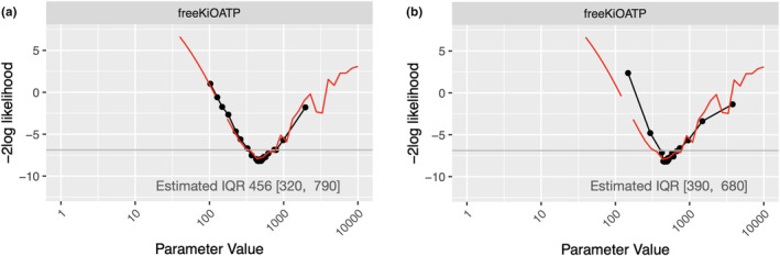
Comparison of the profile likelihood of inhibition constant (freeKiOATP) of the PBPK model for DDI of pitavastatin and rifampicin ¹¹ (Example 1) drawn using the proposed method and the conventional method. The black line is the approximate profile likelihood drawn using the proposed method. Red is the profile likelihood using the conventional method. (a) Approximate profile likelihood drawn with an additional CGNM iterations which took 3.7 min. (b) Approximate profile likelihood drawn without any extra model evaluation (hence it took around 1.1 s). CGNM, Cluster Gauss‐Newton method; DDI, drug‐drug interaction; IQR, interquartile range; PBPK, physiologically‐based pharmacokinetic.

The conventional approach took around 3 h after parameter estimation to compute profile likelihood when using the LM method as the optimization method with the best‐fit parameter found by the CGNM as the initial iterate of LM. Note that if the LM method is started from an arbitrary initial estimate, it failed to converge, as can be seen in Figure S4.

Figure 3 shows the 2D profile likelihood drawn using the proposed method. For ease of visualizability, we are only showing the part that is below the threshold of the chai squared distribution with a degree of freedom of 2 and alpha of 0.25. To draw 2D profile likelihood, it only took 1.7 s. In Figure 3, we can clearly see the parameter‐parameter correlations. From Figure 3, we have observed a clear linear parameter‐parameter relationship of the product of fraction absorbed and intestinal availability (FaFg), and fraction of the drug that is excreted via bile (fbile). In fact, the slope of this linear relationship is observed to be close to one and based on this observation we have built a hypothesis that we can reparametrizing the model with FaFg + fbile as one of the parameters. To investigate this, one could reparameterize the model and conduct the profile likelihood; however, we can do ad hoc reparameterization for the parameter combinations with the known likelihood (based on the model evaluations during the CGNM iteration) and then apply the proposed method to produce approximate profile likelihood. In other words, we make use of the fact that likelihood is invariant with respect to the parameter transformation so that we can construct approximate profile likelihood of the reparameterized model without conducting new estimation or model evaluation. As can be seen in Figure 4a, we were able to draw an approximate profile likelihood of FaFg + fbile based on the CGNM parameter estimation, where FaFg and fbile are parameterized as separate parameters in 0.5 s. Figure 4b shows the profile likelihood of FaFg + fbile obtained using the reparameterized model where FaFg + fbile and fbile are the parameters together with the other five parameters (i.e., FaFg + fbile, fbile, Beta, CLintall, freeKiOATP, Ka, and ksto are the parameters of the model). Although Figure 4a,b are not identical, the general shape is preserved.

FIGURE 3.

A two‐dimensional approximate profile likelihood of the PBPK model for DDI of pitavastatin and rifampicin ¹¹ (Example 1) drawn using the proposed method (took 1.7 s). We can observe various parameter‐parameter relationships, one of the most noticeable ones is the linear relationship between fbile and FaFg. In fact, the slope of this linear relationship can be observed to be close to one from this plot. DDI, drug‐drug interaction; PBPK, physiologically‐based pharmacokinetic.

FIGURE 4.

Approximate profile likelihood of the composite parameters fbile + FaFg of the PBPK model for DDI of pitavastatin and rifampicin ¹¹ (Example 1). (a) Post hoc reparameterization, where the CGNM computation that estimated fbile and FaFg as separate parameters, and then when drawing approximate profile likelihood, reparameterized in post hoc manner (hence no additional model evaluation and took 0.5 s to draw this plot). (b) Approximate profile likelihood drawn based on the CGNM computation of the reparameterized model where fbile + FaFg is one of the unknown parameters (3.9 min). CGNM, Cluster Gauss‐Newton method; DDI, drug‐drug interaction; PBPK, physiologically‐based pharmacokinetic.

Example 2

To illustrate how approximate profile likelihood can be used to discuss the sensitive parameters, we have applied the proposed method to the PBPK model of an endogenous biomarker for OATP‐mediated DDI, coproporphyrin I (CP‐1). Yoashikado et al. ¹¹ state that “three parameters out of eight, CL_int,all (overall intrinsic clearance), v _syn (rate of biosynthesis of CP‐1), and K _i,u,OATP (OATP1B inhibition constant) were characterized as relatively sensitive.”

Figure 5 depicts the approximate profile likelihood of all eight parameters of the CP‐1 PBPK model. As can be seen clearly from Figure 5, three parameters Yoshikado et al. have identified is sensitive with respect to the likelihood; that is to say, they are sensitive parameters with respect to the model fit. In addition, given approximate profile likelihood is the upper bound of the true profile likelihood, according to the criterion in Wieland et al., ¹² one can conclude that the other five parameters are not identifiable.

FIGURE 5.

Profile likelihoods of the PBPK model of an endogenous biomarker for OATP‐mediated DDI, coproporphyrin I (CP‐1) ¹¹ (Example 2) drawn using the proposed method (took 1.2 s) and the conventional method (took 2.8 h). CGNM, Cluster Gauss‐Newton method; DDI, drug‐drug interaction; LM, Levenberg‐Marquardt; PBPK, physiologically‐based pharmacokinetic.

This example demonstrates that even though the model itself is unidentifiable (i.e., not all unknown parameters can be estimated from the data), the parameter of interest—the OATP1B inhibition constant—can indeed be estimated from the available data. This observation further substantiates the conclusions drawn in the original paper. ¹¹

Compared to the conventional method, the approximate profile likelihood is significantly faster, taking just 1.2 s versus the 2.8 h required by the conventional —LM‐based method. As depicted in Figure 5, the profile likelihoods around the maximum likelihood are virtually identical between the two methods. However, there is a noticeable deviation as they move away from the maximum likelihood. Consequently, the profile likelihood drawn using both methods are nearly identical for the unidentifiable parameters (Beta, FaFg, fbile, freeKiMRP2, and fsyn). In a manner similar to Example 1, as shown in Table S4, the interquartile ranges of the identifiable parameters are smaller when estimated using the approximate profile likelihood compared to the conventional method. Nonetheless, the results are reasonably comparable for rough estimation purposes.

Example 3 (identifiability analyses using approximate profile likelihood)

To further verify the use of approximate profile likelihood for the identifiability analyses, we have applied the proposed method to the PBPK‐TMDD model of bosentan published in Koyama et al. ²³ Koyama et al. claim that “the target binding parameters were identifiable only if the observations from the lowest dose (10 mg) were included.”

Figure 6a depicts the approximate profile likelihood where plasma concentration data from 10, 50, 250, 500, and 750 mg arms were included in the model fit.

FIGURE 6.

Profile likelihood of the PBPK‐TMDD model of bosentan ¹² (Example 3) drawn using the proposed method and the conventional method. (a) Plasma concentration data from the 10, 50, 250, 500, and 750 mg arms were included in the model fit. (b) Plasma concentration data from the 50, 250, 500, and 750 mg arms were included in the model fit. (c) Plasma concentration data from the 250, 500, and 750 mg arms were included in the model fit. CGNM, Cluster Gauss‐Newton method; LM, Levenberg‐Marquardt; PBPK, physiologically‐based pharmacokinetic; TMDD, target‐mediated drug disposition; V _max, maximum value.

As can be seen in Figure 6a, all eight parameters are identifiable from the data. However, as can be seen in Figure 6b, when fitting only with the 50, 250, 500, and 750 mg arms (without 10 mg arm), K_off (dissociation constant of target binding) becomes practically unidentifiable and, as can be seen in Figure 6c, when fitting only with the 250, 500, and 750 mg arms (without the 10 and 50 mg arms) K_off and Kd (dissociation equilibrium constant) become unidentifiable.

This result clearly illustrates that the plasma concentration data from the lower doses are vital for estimating parameters related to receptor occupancy, which aligns with the assertions made in the original paper. ²³

In comparison to the conventional method, a similar trend—as observed in Examples 1 and 2—is evident in this example as well, with a better approximation nearer to the maximum likelihood. This also applies to the interquartile ranges, as tabulated in Tables S2–S4. A notable deviation occurs in the identifiability of K_off, where plasma concentration data from the 10, 50, 250, 500, and 750 mg arms were incorporated into the model fit (Table S2). The upper bound of the interquartile range appears to be outside where the profile likelihood is calculated using the conventional method, whereas it is otherwise in the approximate profile likelihood. This is yet another instance showcasing that the approximate profile likelihood acts as an upper bound of the profile likelihood, thus leading to an underestimation of the interquartile range.

DISCUSSION

In this paper, we have shown that we can approximate profile likelihood using the intermediate model evaluations of CGNM parameter estimation. Thus, after the CGNM parameter estimation, profile likelihood can be approximated without any extra model evaluation, hence, almost with no additional computation time. We believe this computationally efficient way of approximating profile likelihood can be especially beneficial at the model building stage. To shorten the model development cycle, we often omit drawing profile likelihood in the earlier stage of the model building. However, considering mechanistic models are often unidentifiable, it is beneficial to visually understand parameter identifiability of each parameter and also the parameter‐parameter correlations. Hence, we believe having a quick way to approximate profile likelihood will be a beneficial model diagnostic tool that can be used during an early stage of building mechanistic models, such as PBPK models.

The proposed method is possible because CGNM starts from randomly distributed initial iterates and search through the likelihood surface. Given this characteristic of CGNM, to some extent, the full likelihood (at least within the range of the initial parameter distribution) is well‐characterized; hence, its lower dimension projection, profile likelihood, can be drawn. As a consequence, we can obtain the profile likelihood of all parameters, and we can also conduct post hoc reparameterization and obtain approximate profile likelihood.

Given that the parameter search is conducted following the CGNM algorithm, the density of points in the parameter space where the likelihood is evaluated during the iteration (hence, the points used to approximate profile likelihood using the proposed method) are biased toward best‐fit parameter combinations as can be seen in Figures S2–S4. This bias could cause some approximation error or unfavorable resolution away from the maximum likelihood; however, it contributes to the computational efficiency and good resolution near the maximum likelihood. Note that to rigorously characterize full likelihood, one would need an exhaustive sampling where the computation cost increases rapidly as the number of the dimension of the parameter space increases. For illustrative purposes, we generated 2500 uniformly distributed random parameter combinations, evaluated the likelihood for each of the parameter combination, and then used to the proposed algorithm (using this uniform distribution instead of distribution created during CGNM iteration) to draw approximate profile likelihoods. However, as Figures S5–S7 indicate, it fails to approximate the profile likelihood. This observation shows the crucial advantage of reusing the parameter distribution generated during the CGNM iteration, for drawing relevant approximate profile likelihoods.

It is worth noting that a similar approach to plotting the profile likelihood could potentially be applied using the parameter distribution derived from other parameter optimization algorithms. For instance, we implemented the proposed algorithm on parameter distributions obtained during the iterations of the Genetic Algorithm. ²⁴ As depicted in Figures S8–S10, this approach was reasonably successful for some identifiable parameters. However, for nonidentifiable parameters, it was not as effective as when leveraging the distribution acquired via CGNM. The fundamental objective of CGNM is to obtain multiple minimizers for the nonlinear least squares problem. In essence, it presupposes the model as unidentifiable, implying that certain parameters should exhibit a “flat” profile likelihood. This predisposition can enhance the proposed methodology's ability to approximate the profile likelihood.

Through our example, we have shown that profile likelihood generated using intermediate computation of CGNM is a reasonable estimate of profile likelihood that is obtained by repeatedly applying the conventional optimization algorithm. We claim that despite the approximate profile likelihood drawn using the proposed method may lack resolution at some points, the general feature of the profile likelihood is captured at the usable level. It is especially noteworthy that the proposed method can give a profile likelihood of all the model parameters, whereas the conventional method will require to repeat the procedure for each parameter. It is worth noting, as depicted in Figures 1, 5 and 6, that the profile likelihoods obtained through the LM method frequently exhibit a lack of smoothness. This irregularity is largely attributable to the suboptimal convergence associated with the LM method. The presented results were obtained after a series of iterative adjustments to the settings of the LM method. Therefore, for those that require more robust “true” profile likelihoods, it may be necessary to engage with more sophisticated optimization methods, which most likely will cost even more computation time.

In addition, we have shown that we can re‐run the CGNM parameter search while fixing the initial distribution of the parameter we wish to draw profile likelihood to refine the profile likelihood. This refinement of profile likelihood using CGNM was significantly faster than the conventional method. Although we only compared with the simple LM method, this advantage in the computation speed of CGNM is extensively discussed in ref. [1], thus we here will not further discuss this.

Although we have emphasized that the profile likelihood determined using our proposed method is approximate, it still enables conclusions about parameter unidentifiability. This reasoning stems from the fact that the approximate profile likelihood serves as the upper limit of the true profile likelihood. If the approximate profile likelihood remains flat and consistently below a given statistical threshold (for instance, as illustrated in our example using the chi distribution with α = 0.25), one can infer that the parameter is unidentifiable within the specific domain. On the other hand, if the approximate profile likelihood suggests that a parameter is identifiable, it may not actually be so. Thus, we recommend further computations if the identifiability of a particular parameter is crucial. We have visually represented this rationale in a schematic drawing in Figure S11.

In this study, we conducted 39 identifiability analyses spanning three models and five datasets (Table 1, Tables S2–S4). Of these, only in one instance did the approximate profile likelihood differ from the conventional method (refer to the identifiability analysis of K_off in Table S2; the associated approximate profile likelihood is depicted in Figure 6a and Figure S12a). In this unique case, the approximate profile likelihood erroneously deemed the parameter identifiable when it was not. Figure S12b displays the profile likelihood for this parameter post additional CGNM computation, adjusting for this parameter distribution. The result aligns closely with the profile likelihood obtained using the conventional algorithm.

In summary, we propose the following workflow:

1. Robustly obtain best‐fit parameter combinations using CGNM.

2. Draw profile likelihood for all parameters using the proposed method.

3. Divide the parameters into unidentifiable parameters and possibly identifiable parameters.

4. Draw 2D profile likelihood using the proposed method to investigate parameter‐parameter correlations and consider possible reparameterization.

5. Draw profile likelihood of reparametrized model using the proposed method by post hoc reparameterization without re‐estimation of the reparametrized model.

6. Use CGNM to refine profile likelihood for the parameter where one wishes to have high‐resolution profile likelihood or accurate confidence interval.

Last, we wish to illustrate some limitations of the approximate profile likelihood and its current implementation. First, as we have been emphasizing through name and description, it is an approximation, and, rigorously speaking, the upper‐bound of the actual profile likelihood. In addition, as can be seen in the first example, the resolution and accuracy of the approximate profile likelihood are in the trade‐off relationship. Thus, by refining the resolution by increasing the number of quantiles (in step 6–1 of the pseudo algorithm) the approximate profile likelihood may become non‐smooth due to the artifact of the approximation. In addition, we focused our attention to the PBPK model of our interest; however, investigation to validate and improve the proposed algorithm may be of interest to more complex models, such as a Quantitative Systems Pharmacology models. As CGNM is an algorithm to solve the nonlinear‐least squares problem, in this paper, we only considered fixed effect models. Given the discussion of the identifiability seems to be an active area of interest for nonlinear mixed effect models ²⁵ further investigation to extend the proposed method to such models may be of interest.

CONCLUSION

We have shown that we can draw approximation of profile likelihood almost for “free” (i.e., without no additional model evaluation) by reusing computation done during the parameter estimation via CGNM. The obtained profile likelihood can be used for parameter identifiability analyses. Together with the previously published results on the computation efficiency and robustness of CGNM, we claim that CGNM is a convenient method to conduct parameter estimation, profile likelihood, and identifiability analyses of complex mechanistic models.

AUTHOR CONTRIBUTIONS

Both authors wrote the manuscript, designed the research, performed the research, and analyzed the data.

FUNDING INFORMATION

This work was supported by a Grant‐in‐Aid for Scientific Research (B) (22H02789 to Y.S.) from the Japan Society for the Promotion of Science (JSPS).

CONFLICT OF INTEREST STATEMENT

The authors declared no competing interests for this work.

Supporting information

Appendix S1

Appendix S2

Appendix S3

Appendix S4

Aoki Y, Sugiyama Y. Cluster Gauss‐Newton method for a quick approximation of profile likelihood: With application to physiologically‐based pharmacokinetic models. CPT Pharmacometrics Syst Pharmacol. 2024;13:54‐67. doi: 10.1002/psp4.13055

REFERENCES

- 1. Aoki Y, Hayami K, Toshimoto K, Sugiyama Y. Cluster Gauss–Newton method: an algorithm for finding multiple approximate minimisers of nonlinear least squares problems with applications to parameter estimation of pharmacokinetic models. Optim Eng. 2020;23:169‐199. [Google Scholar]
- 2. Aoki Y, Hayami K, Sterck HD, Konagaya A. Cluster Newton Method for sampling multiple solutions of underdetermined inverse problems: application to a parameter identification problem in pharmacokinetics. SIAM J Sci Comput. 2014;36(1):B14‐B44. [Google Scholar]
- 3. Niu J, Nguyen VA, Ghasemi M, Chen T, Mager DE. Cluster Gauss–Newton and CellNOpt parameter estimation in a small protein signaling network of vorinostat and bortezomib pharmacodynamics. AAPS J. 2021;23:1‐15. [DOI] [PMC free article] [PubMed] [Google Scholar]
- 4. Yoshida K, Maeda K, Kusuhara H, Konagaya A. Estimation of feasible solution space using Cluster Newton Method: application to pharmacokinetic analysis of irinotecan with physiologically‐based pharmacokinetic models. BMC Syst Biol. 2013;7(3):1‐11. [DOI] [PMC free article] [PubMed] [Google Scholar]
- 5. Fukuchi Y, Toshimoto K, Mori T, et al. Analysis of nonlinear pharmacokinetics of a highly albumin‐bound compound: contribution of albumin‐mediated hepatic uptake mechanism. J Pharm Sci. 2017;106(9):2704‐2714. [DOI] [PubMed] [Google Scholar]
- 6. Asami S, Kiga D, Konagaya A. Constraint‐based perturbation analysis with Cluster Newton Method: a case study of personalized parameter estimations with irinotecan whole‐body physiologically based pharmacokinetic model. BMC Syst Biol. 2017;11:151‐162. [DOI] [PMC free article] [PubMed] [Google Scholar]
- 7. Toshimoto K, Tomaru A, Hosokawa M, Sugiyama Y. Virtual clinical studies to examine the probability distribution of the AUC at target tissues using physiologically‐based pharmacokinetic modeling: application to analyses of the effect of genetic polymorphism of enzymes and transporters on irinotecan induced side effects. Pharm Res. 2017;34:1584‐1600. [DOI] [PMC free article] [PubMed] [Google Scholar]
- 8. Kim SJ, Toshimoto K, Yao Y, Yoshikado T, Sugiyama Y. Quantitative analysis of complex drug–drug interactions between repaglinide and cyclosporin a/gemfibrozil using physiologically based pharmacokinetic models with in vitro transporter/enzyme inhibition data. J Pharm Sci. 2017;106(9):2715‐2726. [DOI] [PubMed] [Google Scholar]
- 9. Nakamura T, Toshimoto K, Lee W, Imamura CK, Tanigawara Y, Sugiyama Y. Application of PBPK modeling and virtual clinical study approaches to predict the outcomes of CYP2D6 genotype‐guided dosing of tamoxifen. CPT Pharmacometrics Syst Pharmacol. 2018;7(7):474‐482. [DOI] [PMC free article] [PubMed] [Google Scholar]
- 10. Mochizuki T, Aoki Y, Yoshikado T, et al. Physiologically‐based pharmacokinetic model‐based translation of OATP1B‐mediated drug–drug interactions from coproporphyrin I to probe drugs. Clin Transl Sci. 2022;15(6):1519‐1531. [DOI] [PMC free article] [PubMed] [Google Scholar]
- 11. Yoshikado T, Aoki Y, Mochizuki T, et al. Cluster Gauss‐Newton Method analyses of PBPK model parameter combinations of coproporphyrin‐I based on OATP1B‐mediated rifampicin interaction studies. CPT Pharmacometrics Syst Pharmacol. 2022;11(10):1341‐1357. [DOI] [PMC free article] [PubMed] [Google Scholar]
- 12. Wieland FG, Hauber AL, Rosenblatt M, Tönsing C, Timmer J. On structural and practical identifiability. Curr Opin Syst Biol. 2021;25:60‐69. [Google Scholar]
- 13. Kreutz C, Raue A, Timmer J. Likelihood based observability analysis and confidence intervals for predictions of dynamic models. BMC Syst Biol. 2012;6(1):1‐9. [DOI] [PMC free article] [PubMed] [Google Scholar]
- 14. Lee W, Kim M, Kim J, Aoki Y, Sugiyama Y. Predicting in vivo target occupancy (TO) profiles via PBPK‐TO modeling of warfarin pharmacokinetics in blood: importance of low dose data and prediction of stereoselective target interactions. Drug Metab Dispos. 2023;51:1145‐1156. [DOI] [PubMed] [Google Scholar]
- 15. Aoki Y. CGNM: Cluster Gauss‐Newton Method . 2023. R package version 0.6.2. https://CRAN.R‐project.org/package=CGNM.
- 16. Murphy SA, Van der Vaart AW. On profile likelihood. J Am Stat Assoc. 2000;95(450):449‐465. [Google Scholar]
- 17. R Core Team . R: A Language and Environment for Statistical Computing. R Foundation for Statistical Computing; 2021. https://www.R‐project.org/. [Google Scholar]
- 18. Elzhov TV, Mullen KM, Spiess A‐N, Bolker B. minpack.lm: R Interface to the Levenberg‐Marquardt nonlinear least‐squares algorithm found in MINPACK, plus support for bounds. 2016. R package version 1.2‐1. https://CRAN.R‐project.org/package=minpack.lm
- 19. Marquardt DW. An algorithm for least‐squares estimation of nonlinear parameters. J Soc Indust Appl Math. 1963;11(2):431‐441. [Google Scholar]
- 20. Moré JJ. The Levenberg‐Marquardt algorithm: implementation and theory. In: Numerical Analysis: Proceedings of the Biennial Conference Held at Dundee, June 28–July 1, 1977. Berlin, Heidelberg: Springer Berlin Heidelberg. 2006. 105–116.
- 21. Moré JJ, Sorensen DC, Hillstrom KE, Garbow BS. The MINPACK project. In: Cowell WJ, ed. Sources and Development of Mathematical Software. Prentice‐Hall; 1984:88‐111. [Google Scholar]
- 22. Fidler M, Hallow M, Wilkins J, Wang W. RxODE: facilities for simulating from ODE‐based models. 2023. R package version 1.1.5. https://CRAN.R‐project.org/package=RxODE.
- 23. Koyama S, Toshimoto K, Lee W, Aoki Y, Sugiyama Y. Revisiting nonlinear Bosentan pharmacokinetics by physiologically based pharmacokinetic modeling: target binding, albeit not a major contributor to nonlinearity, can offer prediction of target occupancy. Drug Metab Dispos. 2021;49(4):298‐304. [DOI] [PubMed] [Google Scholar]
- 24. Scrucca L. GA: a package for genetic algorithms in R. J Stat Softw. 2013;53(4):1‐37. doi: 10.18637/jss.v053.i04 [DOI] [Google Scholar]
- 25. Duchesne R, Guillemin A, Gandrillon O, Crauste F. Practical identifiability in the frame of nonlinear mixed effects models: the example of the in vitro erythropoiesis. BMC Bioinform. 2021;22:1‐21. [DOI] [PMC free article] [PubMed] [Google Scholar]
Associated Data
This section collects any data citations, data availability statements, or supplementary materials included in this article.
Supplementary Materials