Bistable perception, precision and neuromodulation

Abstract

Bistable perception follows from observing a static, ambiguous, (visual) stimulus with two possible interpretations. Here, we present an active (Bayesian) inference account of bistable perception and posit that perceptual transitions between different interpretations (i.e. inferences) of the same stimulus ensue from specific eye movements that shift the focus to a different visual feature. Formally, these inferences are a consequence of precision control that determines how confident beliefs are and change the frequency with which one can perceive—and alternate between—two distinct percepts. We hypothesized that there are multiple, but distinct, ways in which precision modulation can interact to give rise to a similar frequency of bistable perception. We validated this using numerical simulations of the Necker cube paradigm and demonstrate the multiple routes that underwrite the frequency of perceptual alternation. Our results provide an (enactive) computational account of the intricate precision balance underwriting bistable perception. Importantly, these precision parameters can be considered the computational homologs of particular neurotransmitters—i.e. acetylcholine, noradrenaline, dopamine—that have been previously implicated in controlling bistable perception, providing a computational link between the neurochemistry and perception.

Introduction

Bistable perception ensues from observing an ambiguous stimulus with two possible interpretations e.g. the Necker cube or Rubin’s vase. Here, alternation of the visual percept arises when the stimulus offers two distinct explanations that cannot be perceived simultaneously (Brascamp et al. 2018). For example, whilst observing the Necker cube, individuals switch between perceiving a cube oriented leftward or rightward. Experimentally, it has been shown that neurotransmitters are crucial for modulating this phenomenon (van Loon et al. 2013)—specifically, implicating catecholaminergic (Pfeffer et al. 2018), dopaminergic (Schmack et al. 2013), cholinergic (Sheynin et al. 2020), and noradrenergic (Einhauser et al. 2008) neurotransmission in modulating the frequency of perceptual switching. The latter work studied noradrenaline indirectly via pupil dilation—see (Larsen and Waters 2018). In our study, we provide a computational account of how these particular neurotransmitters can influence bistable perception. For this, we rely on how their computational homologs—i.e. precision modulation under active (Bayesian) inference (Parr and Friston 2017)—can induce perceptual alternation.

Active inference is a Bayesian formulation of brain function that casts perception and action as “self-evidencing” (Hohwy 2016) or minimizing free energy across time (Friston et al. 2017; Kaplan and Friston 2018; Friston 2019; Da Costa et al. 2020). It characterizes perception as an inferential process (Von Helmholtz 1867; Clark 2013) across the space of all possible hypotheses that could have given rise to a particular stimulus (Friston 2005). These inferences are a consequence of how confident (or precise) beliefs are over particular model distributions. Broadly, such models comprise sequences of “hidden” states or causes which generate observable sensory data. For example, if the probability of a sensory input given its cause is extremely precise, then one can confidently attribute that sensory observation to a particular cause. Contrariwise, an imprecise probability distribution implies an ambiguous association between cause and effect and sensory observations can do little to resolve the uncertainty about their causes. This is precisely why precision control can influence the type of inferences made and induce bistable perception by mimicking the role of specific neuromodulators (Moran et al. 2013; Schwartenbeck et al. 2015; Parr et al. 2018; Vincent et al. 2019).

Here, we use particular precision parameters to investigate the computational mechanisms that underwrite bistable perception. We hypothesized that there are multiple, but distinct, ways in which precision control can interact to give rise to bistable perception. These precision manipulations influence the frequency with which one can perceive (and alternate between) two distinct percepts and speak to an intricate precision balance underwriting bistable perception. Explicitly, we evaluate multiple combinations of precision, over three distinct model distributions that may give rise to bistable perception. These are (i) sensory precision, (ii) precision over state transitions, and (iii) precision over probable action plans, as these are thought to be mediated by acetylcholine (ACh) (Moran et al. 2013; Parr et al. 2018), noradrenaline (Vincent et al. 2019), and dopamine (Schwartenbeck et al. 2015), respectively.

To demonstrate perceptual switching—as a function of various precisions—we instantiate an active inference model of the Necker cube paradigm (Gregory 1980). Here, we will use agent and model to mean one and the same thing. In this example, the agent is presented with an ambiguous, static image, i.e. the Necker cube, and infers its cause, namely, a cube facing either to the right or left. How quickly and often the agent alternates between the two inferred (i.e. perceived) orientations is determined by the confidence with which particular beliefs are updated—modulated by the different precision parameters. We discuss the correspondence between these precision terms, their neuromodulatory homologs and role in facilitating bistable perception in Table 1. Inevitably, these associations are vast oversimplifications. However, they are useful heuristics that appear to be consistent with much of the data on neuromodulatory function.

Table 1.

Overview of precision parameters, and how they may affect bistable perception.

Precision parameter	Neuromodulators	Bistable perception effects	Computational role
Sensory ()	Cholinergic	(Sheynin et al. 2020): increased ACh during bistable perception increased the visibility of individual percepts and decreased the frequency of perceptual transition. (Pfeffer et al. 2018): found no effect of cholinergic release during perception transitions.	Sensory precision positively correlates with the visual accuracy of perceived orientation and negatively with the switch frequency.
State transition ()	Noradrenergic	Catecholamines (i.e. a mixture of dopamine and noradrenaline) negatively correlates with the duration of holding one percept during a multistability task (Pfeffer et al. 2018)	State transition precision modulates the evolution of a perceived orientation, and precise state transitions reduce switch frequency.
Policy ()	Dopaminergic	(Schmack et al. 2013): DRD4-2R (gene) that targets dopaminergic release also influences perceptual switches. However, DRD4-4R and -7R do not show any modulatory effects.	Policy precision is linked to confidence about actions (i.e. eye movements) and can decrease the switch frequency.

Briefly, sensory precision (of the likelihood function) determines the confidence in beliefs about the causes of outcomes. This definition can therefore be read as (selective) attention in psychology (Feldman and Friston 2010; Mirza et al. 2019). In other words, by modulating the sensory precision in a context specific manner, the model can selectively attend to the stimuli that are task-relevant (Mirza et al. 2021). Similarly, precision over state transitions models the volatility of hidden states. If this is extremely precise, the agent would have high confidence about the evolution of states over time. Conversely, with a low state transition precision, the agent’s beliefs about future states would become progressively more uncertain (i.e. high Shannon entropy). Lastly, the precision over probable action plans (i.e. policy selection) determines the confidence in the selected action trajectory or policy. We expected that increasing each of these precisions would decrease the frequency of visual perception alternation induced by precise beliefs over the perceived orientation (or the visual context), independently of the other precision terms. We analyzed the posterior probability of orientation under different precision values. We hypothesized that all three precision terms would induce a similar change in belief updating and the ensuing switch rate (see Table 1). In other words, the differential effects of the precision manipulations were assessed in terms of what the synthetic subject “believed” at the time of each perceptual switch.

This paper is structured as follows. First, we review formal (i.e. computational) accounts of bistable perception. Next, we briefly introduce active inference with a special focus on precision. This provides a nice segue to introduce our generative model for simulating bistable perception of the Necker cube; a canonical paradigm in the bistable perception literature (Kornmeier and Bach 2005; Wernery et al. 2015; Choi et al. 2020). The model is then used to test our hypotheses regarding the multiple and distinct routes through which bistable perception can arise. Finally, we discuss the results to understand how our simulated manipulations of precision relate to neuromodulation in the brain.

Computational accounts of bistable perception

Previously, there have been many attempts to account for bistable perception phenomena ranging from dynamical systems models (Fürstenau 2007, 2010, 2014) through to predictive processing frameworks (Dayan 1998; Hohwy et al. 2008; Brascamp et al. 2018; Leptourgos et al. 2020a; Leptourgos et al. 2020b). The latter explanation includes a formulation (Wang et al. 2013; Sterzer et al. 2017; Weilnhammer et al. 2017; Robinson 2018) that characterize perceptual switches as a consequence of prediction errors emerging from residual evidence for the suppressed percept. In this account, bistable perception emerges from a progressive increase of the prediction error not explained by the extant percept, engendering the alternate explanation (Weilnhammer et al. 2017). We extend this account of bistable perception using active inference. Explicitly, we illustrate that variations in precision (over distinct model parameters) can give rise to bistable perception by influencing how confidently sensory observations are inferred.

Our account is also aligned with another model of bistable perception introduced by Weilnhammer et al. (2021). They observed that bistable perception emerged from a fluctuation in the sensory information available to the brain. This fluctuation can be explained by saccadic suppression—the suppression of sensory pathways during saccades (Crevecoeur and Kording 2017)—and can lead to increased perceptual alternation. Under predictive processing accounts, this suppression relies upon changes in the precision the brain assigns to sensory data at different times during the action-perception cycle. This highlights that eye movements are necessary for understanding bistable perception and can therefore provide behavioral evidence of sensory precision modulations. Importantly, this aligns with our model by demonstrating that bistable perception is (i) modulated via different levels of (sensory) precision and (ii) experimentally linked to eye movements, namely, active vision or inference.

Separately, Parr et al. (2019) used active inference to investigate the computational mechanisms that underwrite bistable perception. They postulated that bistable perception is a consequence of alternations in (covert) attentional deployment toward certain stimulus features when two different percepts may be supported by different stimulus features (e.g. luminance contrast at different places in the visual field). The alternation is a consequence of accumulation of uncertainty about the percept relating to the unattended features. By choosing to deploy attention to resolve this uncertainty, we switch our focus and therefore our percept. The numerical experiments accompanying this hypothesis showed that changes in different precision parameters influenced the frequency of transitions, given the inferences being made. This process has been linked to eye movements focusing on distinct parts of the illusory object, which is in line with a call for active vision formulations of bistable perception (Safavi and Dayan 2022).

Materials and methods

Here, we briefly describe active inference and precision parameters that underwrite the computational mechanisms that may give rise to bistable perception.

Active inference

Active inference, a corollary of the free energy principle, is a formal way to describe the behavior of self-organizing (dynamical) systems that interact with an external environment. It postulates that these systems self-organize by minimizing their surprisal about sensory observations (), i.e. maximizing their (Bayesian) model evidence (Friston et al. 2010; Sajid et al. 2022) or “self-evidencing”(Hohwy 2016). Surprisal is the negative logarithm of an outcome probability, i.e. −ln P(o). Formally, this involves the optimization of a free energy functional i.e. an upper bound on surprisal (Beal 2003; Da Costa et al. 2020; Sajid et al. 2021). This functional can be decomposed in terms of complexity and accuracy, and its minimization thus means finding an accurate explanation for sensory observations that incurs the least complexity cost:

(1)

Here, D_KL is the Kullback–Leibler divergence measuring a statistical distance between two distributions, and refer to the outcome and hidden states (or causes), respectively. Free energy depends upon a generative model that comprises a probability distribution that describes the joint probability of (unobserved) causes and (observed) consequences. This generative model is usually specified in terms of a (likelihood) mapping from hidden causes to outcomes and priors over the hidden causes. The approximate posterior distribution Q in (1) expresses the (posterior) probabilities of hypotheses about hidden states, based on the agent’s observations. Uncertainty about anticipated observations is reduced by selecting those policies (i.e. probable action trajectories) that minimize their expected free energy (G) (Parr and Friston 2019):

(2)

where π refers to a policy, and t is a (future) time-step. G(π) is the sum of G(π, t) for each future time-step. For the purposes of this paper, in which our agent considers only the next point in time, this sum has only one term—i.e. G(π) = G(π, t). The expected free energy equips the agent with a formal way to assess different policies in terms of how likely they are to fulfill an agent’s preferences and information gain about the hidden states of the world. Variational free energy (F) scores the ability of the agent's generative model to explain observed outcomes, whereas the expected free energy (G) quantifies the free energy of outcomes in the future, expected under a particular policy or action. A policy is then selected based on the expected free energy of each policy, which is modulated by the precision parameter :

(3)

where σ refers to the softmax function. Thus, the higher the value of , the more precise beliefs about actions. In other words, policy selection becomes more confident. In summary, active inference dictates that (variational and expected) free energy is minimized under a particular model of the environment i.e. a generative model (Friston et al. 2017). These generative models encode particular hypotheses about the current states of affairs. Practically, the agent represents a joint probability over policies, model parameters, and likelihood and transition functions, respectively:

(4)

The parameter encodes the probability distribution of state–outcome pairs (i.e. likelihood distribution), and encodes the probability distribution of hidden states transitions (i.e. the transition distribution). Both are specified as categorical distributions. Precision terms are inverse temperature parameters. With high precision, the category with the highest probability converges to 1, whereas for low precision, categories tend to have equal probability (Parr and Friston 2017; Sajid et al. 2020b). The above probability distributions describe transitions between states in the environment that generate outcomes. Their transitions depend on actions, which are sampled from the posterior beliefs over the policies. Consequently, the sampled actions change the state of the world, giving rise to new outcomes; and continuing the perception-action loop. For the purposes of this paper, we will assume priors over the precision parameters are themselves infinitely precise. This means that the precision value is constant throughout a trial. For more mathematical details of Equation 4, see Supplementary Materials (A) and Table S1.

Precision modulation

We posit that these precision parameters () can independently modulate bistable perception, since they can shape perceptual confidence and the frequency with which the inferred state of the world alternates. is the sensory precision over the probabilities of the likelihood distribution in the generative model, where (hidden) states map onto observations. Thus, sensory precision expresses the confidence with which the model can infer a cause from observations. Practically, high precision (e.g. ) ensures the model can be confident that a particular outcome will be generated reliably by the latent state. Conversely, low precision (e.g. ) implies an ambiguous relationship between causes and outcomes—and observations do little to resolve uncertainty about their causes. The probabilistic mapping from the current state to the next is denoted by the state transition matrix . The term encodes the precision of the state transition matrix and it expresses the confidence with which the model can predict the present from the past. Precision over beliefs about policies is encoded by , which corresponds to the models' ability to confidently select the next action.

We hypothesized that the increase of all three precision terms would lead to a decreased perceptual transition frequency. Furthermore, we hoped to address how to distinguish the influence of each precision term (i.e. neuromodulators) on bistable perception via frequency of eye movements, acuity (measured using post-switch perceptual confidence), and, finally, via the modulatory effects on neuronal responses encoding distinct percepts of the Necker cube.

Precision and neuromodulatory systems

These precision parameters have previously been associated with specific neuromodulatory systems (Parr and Friston 2017; Parr et al. 2018; Sajid et al. 2020a)—see (Table 1). Briefly, sensory precision (), state transition precision (), and policy precision () can be read as cholinergic, noradrenergic, and dopaminergic neurotransmission, respectively. Some empirical studies suggest a link between the cholinergic release and (the frequency of) perceptual transition. For example, Sheynin et al. (2020) demonstrate that enhanced potentiation of ACh transmission attenuates perceptual suppression during binocular rivalry. Similarly, increased noradrenergic release has also been associated with an altered frequency of perceptual fluctuations (Pfeffer et al. 2018). Pfeffer et al. (2018) demonstrate that high catecholamine levels altered the temporal structure of intrinsic variability of population activity and increased the frequency of perceptual alternations induced by ambiguous visual stimulus. Finally, dopaminergic alteration has also been associated with faster perceptual transition frequency (Schmack et al. 2013).

Simulations of Necker cube paradigm

In the remaining sections, we model bistable perception, and the intricate precision balance that undergirds it, using simulations of the Necker cube paradigm. A key finding of Einhäuser et al. (2004) was that eye movements shift toward the dominant orientation before the perceptual shift. This implies that the perceptual shift is caused by the new visual data acquired following an eye movement. Similarly, the time-discretization—implicit in the active inference scheme—involves a sequence of (perceptual) belief updates interspersed with actions. This emulates the finding of Einhäuser et al. (2004); in that the perceived switch takes place after the (saccadic) action, when the focus of visual sampling has changed. It also complements this finding, in that the saccades are themselves selected upon the basis of the perceptual inference made during the last fixation.

A generative model of the Necker cube

Our generative model of the Necker cube paradigm has two hidden states: fixation point and orientation, and two outcome modalities: where and feature (Fig. 1). The hidden state fixation point has three levels representing bottom-left, top-right, initial position fixation locations, and the orientation state has two levels representing left and right orientation. These fixation point locations are motivated by Einhäuser et al. (2004) and Choi et al. (2020), who observed eye movements between these particular fixation points during perceptual switches. The outcome where reports the location of the eye-fixation: initial, top-right, or bottom-left. The outcome feature reports the corner of the cube being observed: Corner 1 (C1), Corner 2 (C2), or neither (labeled as null).

Fig. 1.

A graphical representation of the Necker cube model. the figure provides a graphical illustration of the generative model with two hidden state factors and two outcome modalities. The first hidden state, the fixation point, has three levels: bottom-left, top-right, and initial fixation (IF). The second hidden state, orientation, has two levels, right and left orientation. The outcome modality features has three levels: “Corner 1” (C1), “Corner 2” (C2), and Null. Here, C1 and C2 denote the two opposite corners and their surrounding areas, and the Null outcome is only plausible under the initial fixation point at the first time-step. There is an identity mapping from fixation point hidden factor to where outcomes. The likelihood function of the generative model, i.e. the probability of an outcome given a hidden state, is encoded such that (i) the bottom-left fixation point is more informative about the right orientation as the agent perceives the related C1 corner, (ii) the top-right fixation point is more informative about left orientation as the agent perceives the related C2 corner there, and (iii) the IF mapped onto a null outcome (i.e. neither C1 nor C2). The fixation point transitions (i.e. representing the state transitions across time) are completely precise. This encodes the eye movements between different fixation locations. Conversely, orientation transitions for the generative process are noncontrollable and transition to the same orientation over time. Here, is a small number that prevents numerical overflow.

The likelihood function maps states to outcomes (i.e. state–outcome pairs). Here, the feature likelihood is dependent on both fixation point and orientation factors. For the generative process (i.e. the process we used to generate the observations during simulation), the where likelihood depends only on the fixation point factor. Therefore, it generates outcomes independently of the orientation state. Conversely, the generative model’s where likelihood depends on both fixation point and orientation factors and explicitly maps each fixation point to a specific orientation (see Fig. 1). Thus, the bottom-left (top-right) fixation location is only plausible under left (right) orientation. Next, we equipped the model with control states (i.e. states whose transition depend on actions) over eye movements via the fixation point factor. Thus, it can control whether to fixate over the top-right, bottom-left, or initial fixation point. The orientation transition is not controllable and the mapping between current and future states was expressed such that the left (right) orientation always transitions to the left (right) orientation (Fig. 1).

Furthermore, the agent was equipped with strong preferences (measured in nats, i.e. natural units) for avoiding the null outcome (−20 nats): see Fig. 3. This was to encourage the agent to sample bottom-left and top-right locations—as the eye movements between these locations have been shown to be associated with perceptual transitions in the Necker cube paradigm (Einhäuser et al. 2004; Choi et al. 2020). At each time point, the agent could choose from three different actions (i.e. 1-step policy) of either fixating at the initial, bottom-left, or top-right location. The prior beliefs about the initial states were initialized to 0.5 for the left and right orientations, 1 for the initial fixation point and zero otherwise.

Fig. 3.

An example trial with 32 time-steps. The first row represents the posterior probability for the hidden state orientation. The second row shows which actions, i.e. eye movements, have been selected (cyan dots) and the posterior probability of each policy. This has only 31 time-steps as actions are modeled for the next step. The last row depicts the sampled outcomes over time with cyan dots and the preferences over outcomes with different shades in the background. Here, the light and dark shades illustrate that the agent has a strong aversion for the Null outcome (−20 nats) observed only at the IF point but has a relatively higher preference for the C1 and C2 outcomes observed at the bottom-left and top-right locations, respectively. A perceptual switch is highlighted using the red dashed boxes, where the red arrow in the second row shows that the switch is (mostly) accompanied with an action toward the preferred fixation point. The red box in the last row shows that observing the outcome C1 facilitated the perceptual switch from the left to the right orientation in this instance, as shown in the first row. The example simulation is for the following precision combination: .

Precision and perceptual alternation

The Necker cube generative model was used to demonstrate the computational mechanisms that underwrite bistable perception. For this, we simulated 729 models with different combinations of the three precision parameters: sensory precision (), state transition precision (), and policy precision (). The precision values used are specified in Table 2.

Table 2.

Precision (hyper-) parameters used to simulate bistable perception. These range from high to low precision values.

Precision parameter	Values
Sensory	0.001, 0.01, 0.1, 0.2, 0.5, 1, 2, 5, 10
State transition	0.001, 0.01, 0.1, 0.2, 0.5, 1, 2, 5, 10
Policy	0.001, 0.01, 0.1, 0.2, 0.5, 1, 2, 5, 10

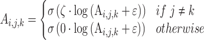
ζ is the sensory precision associated with the likelihood distribution A, i.e. which (hidden) states gave rise to particular observations (where ε = 8 is a small number that prevents numerical overflow):

(5)

Where i represents the outcomes, and j and k represent the orientation (either left or right) and fixation point (either bottom-left or top-right) factors, respectively. For more details on the description of expressions used in the following equations, see Table S1 in supplementary materials. Note, we have excluded the initial fixation point for clarity, as its likelihood matrix is uninformative in the generative model. The two factors are unequal either in combination of the bottom-left fixation point and the right orientation or the contrary (see Fig. 2). The bold A represents the likelihood matrix of how the data are generated (i.e. precise mappings from states to where and feature outcomes). Here, the precision parameter ζ modulates only the columns for the preferred orientation under a given fixation point [i.e. bottom-left fixation point (labeled as 1) maps to the right orientation (labeled as 2) and vice versa], whereas the unpreferred orientation is parameterized as a uniform distribution. Adjusting the columns of the likelihood matrix in this way can be regarded as manipulating the relative sensitivity of neuronal populations—encoding the probability of each possible (hidden) state to sensory afferents—during model inversion or perceptual inference.

Fig. 2.

A graphical illustration of how different precision values change the likelihood and priors of the generative model. (A) A modulation of the likelihood matrix via the sensory precision (). Each row is for a different fixation point with bottom-left on the first and top-right on the second, where the x-axis represents the orientation states and the y-axis the feature outcomes. (B) This panel shows how the state transition precision () perturbations influence the categorical probability distribution of the orientation transition. The x-axis represents the orientation states at the current time point () and the y-axis the orientation states at the next time point (). Here, low values lead to a flat distribution which limits the capacity to project current beliefs about orientation states to past and future epochs whereas with high the state transition matrix becomes more precise and the capacity to pass messages between epochs increases. (C) An intuition of how the γ parameter modulates the expected free energy G, which is assumed to be [0, 0, 1]' for simplicity. For all plots, the scale goes from white (low probability) to black (high probability), and gray indicates gradations in-between. The key difference to note is how the probability distribution shifts from imprecise to precise mappings as we move from low precision values (e.g. ) to high precision values (e.g. ). Note, and values above 0.5 look visually similar and have been deliberately excluded. Furthermore, the different values have been scaled up to 10 for a visual clarity.

Explicitly, the link between the generative model likelihood distribution and is as follows:

(6)

where the likelihood distribution maps hidden states to outcomes given the sensory precision parameter (ζ) and generative process likelihood distribution (A).

Figure 2A provides a graphical illustration of how the precision parameter values modulate the feature likelihood. Here, the sensory precision parameter () modulates the mapping from orientation states to feature outcomes as a function of location states. Under this parameterization, a high sensory precision (the matrices on the right in both rows in Fig. 2A) leads to a precise likelihood mapping for the state pairs bottom-left location—right orientation and top right location—left orientation. Thus, the agent would attribute C1 to the right orientation under the bottom-left position, and C2 to the left orientation under the top-right position. Conversely, under a low sensory precision, the likelihood mapping from an orientation and location to feature outcomes becomes imprecise (left panels in Fig. 2A). With this mapping, the agent could not disambiguate between the causes of C1 and C2 outcomes via the perceived orientation regardless of the sampled fixation position. We motivate our choices for these likelihood mappings based on the degree of visibility of the features, assuming that the cube is opaque. Under this assumption, one should not be able to see Corner-1 for a left-oriented cube. Similarly, one should not be able to see Corner-2 for a right-oriented cube (see Fig. 1 for left and right orientations). These assumptions are translated as likelihood mappings over the feature outcomes for the aforementioned orientation and fixation point combinations, whose precision is encoded by .

The probabilistic mapping from the current state to the next is denoted by the state transition matrix . The term encodes the precision of the state transition matrix in the same fashion as the term :

(7)

Where the bold B represents the transition of how the hidden states change and give rise to new observations, which is defined as an identity matrix in the generative process. The B matrix expresses the confidence with which the model can predict the present from the past and the future, and vice versa. Accordingly, the link between the generative model transition distribution and is as follows:

(8)

where the transition distribution maps current hidden states to future hidden states given the transition precision parameter ( and generative process transition distribution ().

Figure 2B provides a graphic illustration of how precision changes the orientation state transition matrix. An increase in the precision of orientation state transitions () leads to a precise mapping between the orientation at the current and next time points (right panel of Fig. 2B). With a precise transition matrix, the agent would expect the orientation remain the same over time. Conversely, under a low precision, the agent would expect the orientation to change frequently (left panel of Fig. 2B).

As shown in Fig. 2C, γ modulates the confidence over eye movement selection. Specifically, when the γ parameter is high, the confidence in actions is greater and thus action selection is more consistent (i.e. the most likely action will be selected). Conversely, a low γ parameter reduces the precision of posterior beliefs about policies, which leads to more stochastic action selection (akin to matching behavior). This is formalized as follows:

(9)

where Г is the gamma distribution, represents the precision (inverse temperature) of beliefs about policies, and is the prior expectation of temperature (inverse precision) of the beliefs about policies.

Perceptual switch definition

Next, we quantified what constituted a perceptual switch. This is necessary for quantifying the number of perceptual transitions given particular precision combinations. Here, a switch is counted when a particular orientation (e.g. left) has a high posterior probability () at the current time point () but a low posterior probability () at the previous time point ():

(10)

In Equation (10), the bold s variables are the probabilities that parameterize our approximate posterior Q(s). Intuitively, this means that a switch is defined as a change from a belief that the left (or right) orientation is most likely to a belief that the right (or left) orientation is most likely. For the purposes of this paper, we used a threshold of 0.5, although one could use a threshold with higher confidence (e.g. 0.6). In that case, the probabilities between 0.4 and 0.6 for a given orientation might be perceived as a probability weighted mixture of lines in two dimensions.

Results

Face-validation

Here, we present a numerical simulation that establishes the face validity of the Necker cube generative model. For this, we simulated the model with arbitrary precision values; specifically, 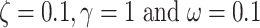(Fig. 3). We observed alternating inferences over the orientation as the trial progressed. This was induced by shifts in eye movements that sampled different corners of the Necker cube. Under our definition, a perceptual switch is observed at time point 7, when both conditions outlined above are met (first row of Fig. 3). Conversely, perceptual switch would not be counted at timestep 2 because the posterior probability over the appropriate orientation at the previous timestep 1 is not but exactly 0.5. Furthermore, this switch is usually accompanied via an action—see middle panel of Fig. 3.

Simulating perceptual switches

Using the criteria in Equation (10), we measured the number of perceptual switches under different precision combinations (Table 2). Each precision combination was simulated 64 times, using random seed initialization, with a trial length of 32 epochs. Figure 4 presents the average number of switches under each precision combination. On average, an increase in precision (regardless of the corresponding model parameter) decreases the number of perceptual transitions independently of other precision terms. For example, as increased from 0.001 to 10, we observed a decrease in the number of perceptual transitions. This is unsurprising given our observation regarding Fig. 2, i.e. beliefs across time are propagated more confidently for high values. Thus, the orientation does not change frequently during the trial and reduces perceptual switches. For ζ, the increased precision gives higher confidence about what is being perceived, thus removing the uncertainty minimizing behavior that would lead to sampling the other fixation point, which could increase the chances of a perceptual switch. It is worth noting, however, that for specific combinations of high ζ and low ω values there is an increase in the number of switches (Fig. 4; upper left and middle figures). Furthermore, decreased precision over policy selection () increases perceptual switches. This is because low values make all policies more likely, leading to a higher frequency of eye movements, and eventual perceptual switch.

Fig. 4.

The average number of switches for different precision combinations. We plot the average number of switches across 32 trials—each comprising of 32 time-steps. Each heatmap is associated with distinct values. The x-axis is associated with and y-axis plots the different value. The average switch count ranges from 0 (dark blue) to 15 (yellow).

The observations above all rest upon a relatively simple insight. For nonzero precision parameters, the best action is always to continue to fixate the same location. This is because the observation associated with our current fixation location supports a belief in a specific orientation (e.g. right orientation if looking at lower left). Under this belief, the alternative location (e.g. upper right) is uninformative as, if the cube were (partially) opaque, there would be little useful visual information there with the opposing corner obscured by the near surface of the cube. In other words, if I am looking to the lower left and infer that the cube is in the right orientation, I would expect that the corner in the upper right will not be visible, so have no reason to look there. As such, the expected free energy will always be lower for the current location compared with alternatives. The result is low switching frequency, with switches that occur only when the action is sampled from the relatively improbable action of moving our eyes. However, the relative improbability of this action is modulated by the precision parameters. Increases in uncertainty about the orientation (via decreases in the sensory or transition precision) attenuate the differences between the expected free energy of each action, resulting in more uncertainty in action selection and increasing the number of switches. The situation is slightly more complicated for the sensory precision parameter, as this has a dual role. The first is in determining the confidence in the orientation (as inferred from potentially unreliable sensory data). The second is in determining the ambiguity (which contributes to the expected free energy) of each location. Decreases in the policy precision attenuate the influence of the expected free energy on action selection, thus making the improbable action relatively less improbable and increasing switching rate. In short, changes in switching rates occur when greater uncertainty favors more stochastic deviations from an optimal policy of maintaining fixation. The greater stochasticity then leads to a greater variability in action selection, as the difference in probabilities between competing fixations is reduced, leading to more opportunities for sampling from the location with a smaller expected free energy. Alternatively, this can also be expressed as selecting policies that minimize ambiguity i.e. expected uncertainty about sensory outcomes given the hidden states: see Equation (2). Thus, a policy with low expected free energy is more likely to be chosen, as it is more likely to furnish precise, unambiguous outcomes.

Dissociating individual precision manipulations

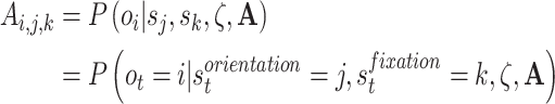
To dissociate the individual influences of each precision during bistable perception, we investigated the (average) posterior probability of the cube’s orientation after the switch occurred—alongside average switch rates. Here, the posterior probability denotes the or value used to identify a switch (Equation (10)). The differences across each precision were evaluated by considering each individually and taking its (marginal) average across all possible combinations (Fig. 5; Table 3). These differences revealed that posterior switch probability and average switch rate for both ζ and ω followed a nonlinear relationship—as modeled with a polynomial expansion (Table 3). Conversely, we observed a negative linear association (i.e. first-order polynomial) for the posterior switch probability and average switch number for γ (Fig. 5A). This highlights that high posterior switch probability (i.e. values ), that determines switch rate, can manifest in multiple ways—see Supplementary Text (B) for further analysis. Furthermore, there is a degenerate (many to one) mapping between the switch posterior probability and number of switches across the different precision terms (Fig. 5C). This speaks to the multiple but distinct routes through which perceptual transitions can arise.

Fig. 5.

Dissociating individual precision terms. For (A) and (B), each data point represents the average switch posterior probability (A; y-axis) and the number of switches (B; y-axis) across different precision values (x-axis). The curves represent the fitted polynomials for each precision value: ζ (blue diamond), ω (green square), and γ (cyan triangle). (C) The joint-plot of the association between number of switches and posterior switch probability. The x-axis presents the posterior switch probability, y-axis the number of switches. Here, each plot presents a different precision term.

Table 3.

Fitted polynomial coefficients across different precision values for posterior switch probability (A) and average switch number (B).

					SSE
A. Posterior switch probability
ζ	***	**	*	-
ω
γ	***	***	-	-
B. Average switch rate
ζ
ω	***	**	*	-
γ	***	**	-	-

The relationship between precision and perceptual switching was modeled with the polynomial expansion: , and its fit was measured using sum of squares of errors (SSE). Here, ^*denotes 10% significance level, ^**denotes 1% significance level, and ^***denotes 0.1% significance level.

Discussion

We investigated how precision manipulation could underwrite bistable perception. For this, we cast bistable perception, the phenomenon where perception alternates between distinct interpretations of a static stimulus, as an enactive process associated with specific eye movements that shift the focus from one visual feature to another leading to a perceptual transition (Einhäuser et al. 2004; Choi et al. 2020). This ensues from a dissociation between the inferred percept and sensory observation (Brascamp et al. 2018) as distinct features of the visual stimulus are sampled. Computationally, we show that the frequency of switches between the two percepts depends on a modulation of (at least) three precision terms that determine the confidence of posterior beliefs. Here, we illustrated that there are distinct ways in which precision (hyper-) parameters—associated with neuromodulators—can interact to affect bistable perception and how their influences can be dissociated from each other using post hoc analysis of posterior beliefs. Below, we relate distinct precision terms to neuromodulators based on the previous literature review (Parr and Friston 2017).

Precision manipulation and neuromodulation

Sensory precision is thought to be modulated via ACh in the active inference framework (Parr and Friston 2017) and in normalization models (Schmitz and Duncan 2018). The influence of this neuromodulator on bistable perception has been studied in Pfeffer et al. (2018) and Sheynin et al. (2020) with apparently inconsistent results of either no influence on the switching rate or decreasing it, respectively. Based on our analysis, we found that sensory precision ζ depends on other precisions when it comes to the switching frequency (Fig. 4) and so looking at the switching rate alone seems insufficient to dissect the specific contribution of this neuromodulator. For this reason, we fitted our simulated data to polynomial expansions to disentangle contribution of individual precision terms. From this analysis, we see that the increase of sensory precision should accentuate the acuity of perceived orientation—assumed to be equivalent to the post-switch perceptual confidence—which is consistent with Sheynin et al. (2020).

The ω precision has previously been associated with noradrenergic release (Parr and Friston 2017). A study by Pfeffer et al. (2018) used a noradrenaline reuptake inhibitor to study this. They found that after administering a drug boosting noradrenaline, participants reported a faster switching rate of a bistable stimulus. As stated above, it is difficult to dissect a specific contribution of neuromodulators (considering them as precision modulators) in bistable perception tasks given only the measure of switching rate. Moreover, bistable perception shows a close link to pupil dilation (Einhauser et al. 2008; Hupé et al. 2009; Kloosterman et al. 2015), which is linked to noradrenergic release (Larsen and Waters 2018), and so future work could target pupil dilation in addition to the eye movements in our current model. However, Brascamp et al. (2021) have shown that only a specific change in pupils is linked to noradrenaline. Thus, the link between the neuromodulation and pupil dilation should be interpreted with caution until connection to bistable perception is further clarified.

We also showed that high policy precision decreases the frequency with which bistable perception alternates. This precision parameter is suggested to be related to dopamine (Parr and Friston 2017), but few studies have looked at the role of dopamine and bistable perception or binocular rivalry. Nevertheless, a study by Schmack et al. (2013) showed that there is an observable alternation of perceptual switches associated with the dopamine receptor D4 (DRD4) gene carriers but this effect was found only for a specific allele (DRD4-2R) but not for others (DRD4-4R and DRD7R). Moreover, Kondo et al. (2012) found no effect of dopaminergic genes on the rate of visual perceptual switches. However, for auditory bistable perception, presence of prominent alleles for synthesizing this neurotransmitter decreased the number of switches. It is also not fully understood how these specific genes affect the dopaminergic neurocircuitry, thus a specific conclusion on whether and how dopamine targets bistable perception is still open.

The three neuromodulators mentioned above are just a small number of all the neuromodulators affecting bistable perception. For instance, it has been shown that psilocybin, a chemical that mostly targets the 5HT2a receptor (i.e. a serotonergic receptor), also modulates perceptual switching (Carter et al. 2005; Carter et al. 2007). Our focus on the other three neuromodulators was motivated by preexisting hypotheses about their roles as mediating precision. However, we hope in future work to use the approach—set out in this paper—to encompass other key neuromodulatory systems.

To test our model, one could use pharmacological drugs to directly manipulate the neuromodulators investigated in our numerical studies. Specifically, to study the cholinergic neurotransmission, one can administer the drug donepezil, as in Sheynin et al. (2020), or rivastigmine that also reduces ACh levels (Sadowsky et al. 2005). Note that although both drugs inhibit acetylcholinesterase, rivastigmine also inhibits butyrylcholinesterase, another enzyme that breaks down acetylcholine. This dual inhibition might give rivastigmine a broader spectrum of action in certain conditions and increased observed behavioral differences compared with donepezil. Similarly, dopaminergic neurotransmission is modulated via the administration of methylphenidate (Gottlieb 2001). These pharmacological interventions can, in principle, be used to test the influence of dopamine on perceptual switch rate, predicted under our model. Finally, noradrenergic neurotransmission can be manipulated using a noradrenaline reuptake inhibitor; for instance, atomoxetine following Pfeffer et al. (2018). These neuromodulatory interventions can also be compared with studies of patients with bipolar disorder, who show both a modulation of the switch rate in bistable perception (Miller et al. 2003; Ngo et al. 2011; Ye et al. 2019), as well as irregularities in all three neuromodulators considered above (Manji et al. 2003). This provides a potential link to studying bipolar disorder through a computational lens, using our paradigm. Interestingly, Leopold et al. (2002) showed that periodical occlusion leads to less switches, which can be related to the transition precision. Whether this also changes the levels of noradrenaline (for instance via pupillometry) might be an interesting future direction to pursue.

Neuroanatomy

The deployment of the precision terms studied here can be associated with feature-based attention (FBA), as the perceptual switches here are understood as switches of orientation. This view is also corroborated with a similarity of brain regions involved in processing bistable perception and FBA, as both activate regions such as frontal eye field, intraparietal cortex, temporoparietal junction, and inferior frontal junction (Brascamp et al. 2018; Zhang et al. 2018; Loued and Preuschoff 2020). Interestingly, all the neuromodulators suggested to be related to distinct precision terms used here are involved in attentional processing (Thiele and Bellgrove 2018). It is possible that the FBA network deploys attentional mechanisms partially by regulating distinct neuromodulators that lead to distinct neurobiological changes but to overlapping behaviors. This relates to the previously reported top-down modulation of bistable perception via the fronto-parietal network (De Graaf et al. 2011).

A range of cortical regions—throughout early visual and attentional networks—have been implicated in multistable perception in general, and the Necker cube specifically. In fact, such paradigms are sometimes used in the search for the neural correlates of consciousness (Sterzer et al. 2009; Blake et al. 2014; Koch et al. 2016; Seth and Bayne 2022); in an attempt to identify brain regions whose activity correlates with subjective experience. This follows from their ability to induce changes in our awareness of different percepts, without changing sensory input. Research has implicated specific dorsal frontal and parietal regions in facilitating these perceptual switches (Inui et al. 2000). These regions are also associated with attentional processing (Vossel et al. 2014), aligning well with our account that highlights the central role of attentional (i.e. precision) modulation in selecting visual information. Supporting the significance of attention in these perceptual processes, early visual pathways have been shown to play a crucial role in generating these perceptual switches (Kornmeier and Bach 2005). However, it's essential to acknowledge a parallel debate in the field concerning the role of the frontal lobe. While some argue that the frontal lobe is actively involved in the perceptual experience itself, others contend that its involvement is more aligned with higher-order processing tasks such as attention and awareness (Safavi et al. 2014; Block 2020; Michel 2022). This ongoing debate, although not exhaustively covered here, adds an additional layer of complexity to our understanding of multistable perception and its neurobiological underpinnings. For greater depth and analysis, readers may wish to refer to Long and Toppino (2004).

Alternative models of eye movements

Our active inference model provides an enactive interpretation of bistable perception; however, the underlying eye movements were deliberately kept simple compared with other models of oculomotor control. Therefore, integrating our model with established eye-movement models may improve predictions of behavioral responses. Here, we review several key frameworks for modeling eye movements.

One possibility is to use Bayesian inference to simulate more involved eye movements relating to gaze fixations. For example, Borji et al. (2013) demonstrated the face-validity of this approach for recognizing visual images. Their model integrates sensory information with top-down models to predict eye movements, using an ideal observer model, like our formulation. Separately, active vision theory also considers the active component to be central component of visual perception, for example the Saliency Map Model (Yoo et al. 2021), Guided Search Model (Wolfe 2021), etc. These models have been used to include more information from action and the kinetics of eye movements, as compared with our discrete-state space formulation. It is worth mentioning that reinforcement learning (RL) models also view eye movements and actions as decisions made by an agent seeking to optimize its performance. Accordingly, some RL schemes are analogous to our formulation, resting on sequential decision-making that optimizes some target distribution; specifically, the expected return (Reichle and Laurent 2006). RL has been used to model saccadic suppression and how it affects visual image displacement (Ziesche et al. 2017).

Limitations and future directions

A key limitation of our work is that we included a limited amount of possible fixation points that makes the study of eye movements over-simplified. Including more fixation points—and thus actions—could provide a more applicable model for empirical studies and fitting of real data. Next, we prespecified the initial probabilities and precision values instead of updating them during each trial. Future work should explore online selection of these precisions and how they influence bistable perception based on a task. This is related to mental actions i.e. internal process that change posterior beliefs by regulating precision (Metzinger 2017; Limanowski and Friston 2018)—and can be added via a hierarchical model in which slower parts of the model modulate the precision terms that influence faster dynamics (Hesp et al. 2021). Understanding how the precision parameters are learned, we could also examine the dynamics of neuromodulators, as so far, we have studied these effects in a stationary environment. Lastly, we focused only on the Necker cube to elucidate bistability. However, other bistable figures—e.g. the Rubin vase—evince a different connection with eye movements. In those instances, eye movements help to disambiguate the percept (Naji and Freeman 2004); instead of inducing ambiguous interpretations. Accordingly, eye movements are not the only actions that should be considered during bistability, but also head movements, as it has been shown that the position of the neck affects bistability (Sato et al. 2022). This is because neck movements can affect ambiguity, even in the absence of eye movements. Thus, bistable perception may also occur in the absence of overt eye movements and could rely upon covert actions, including the deployment of spatial attention—c.f. (Maier and Tsuchiya 2021).

Conclusion

We have shown how bistable switches can be manipulated via three distinct precision terms. Briefly, our formulation provides a two-fold extension of previous models of bistable perception: (i) inclusion of specific overt actions pertaining to eye movements; and (ii) demonstration of a degenerate functional association between model parameters and how they underwrite bistable perception. Moreover, we disentangled among the precision influences, using changes in posterior beliefs to identify perceptual switches. The remaining question concerns the plausible implementation of these precision terms in the brain, which is currently suggested to be related to cholinergic, noradrenergic, and dopaminergic neurocircuitries to state transition, likelihood, and policy selection precision terms, respectively. Overall, our results speak to a degenerate functional architecture that supports the switching rate of bistable perception (Price and Friston 2002; Noppeney et al. 2004; Sajid et al. 2020c) i.e. multiple neuromodulatory systems can modulate the perceptual switching rate.

CRediT author statement

Filip Novicky (Conceptualization, Formal analysis, Investigation, Methodology, Software, Validation, Visualization, Writing—original draft, Writing—review & editing), Thomas Parr (Methodology, Supervision, Writing—review & editing), Karl Friston (Methodology, Software, Supervision, Writing—review & editing), Berk Mirza (Conceptualization, Formal analysis, Investigation, Methodology, Software, Supervision, Writing—review & editing), and Noor Sajid (Conceptualization, Formal analysis, Investigation, Methodology, Software, Supervision, Visualization, Writing—review & editing).

Funding

This work was funded by the Serotonin & Beyond programme (953327 to F.N.), the Medical Research Council (MR/S502522/1 to N.S.), Wellcome Trust (Ref: 203147/Z/16/Z and 205103/Z/16/Z to K.J.F.), and a 2021–2022 Microsoft PhD fellowship (to N.S.). K.J.F. was also supported by a Canada-UK Artificial Intelligence Initiative (Ref: ES/T01279X/1).

 

Conflict of interest statement: None declared.

Software note

The generative model in these kind of simulations changes from application to application; however, the belief updates are generic and can be implemented using standard routines (here spm_MDP_VB_X.m). These routines are available as Matlab code in the SPM academic software: http://www.fil.ion.ucl.ac.uk/spm/. The code for the simulations presented in this paper can be accessed via https://github.com/filipnovicky/Bistable_Perception.

References

- Beal MJ. Variational algorithms for approximate Bayesian inference [PhD. thesis]. University College London; 2003. [Google Scholar]
- Blake R, Brascamp J, Heeger DJ. Can binocular rivalry reveal neural correlates of consciousness? Philos Trans R Soc Lond B Biol Sci. 2014:369(1641):20130211. [DOI] [PMC free article] [PubMed] [Google Scholar]
- Block N. Finessing the bored monkey problem. Trends in cognitive sciences. 2020:24(3):167–168. [DOI] [PubMed] [Google Scholar]
- Borji A, Sihite DN, Itti L. What/where to look next? Modeling top-down visual attention in complex interactive environments. IEEE Trans Syst Man Cybern Syst. 2013:44(5):523–538. [Google Scholar]
- Brascamp J, Sterzer P, Blake R, Knapen T. Multistable perception and the role of the frontoparietal cortex in perceptual inference. Annu Rev Psychol. 2018:69(1):77–103. [DOI] [PubMed] [Google Scholar]
- Brascamp JW, Hollander G, Wertheimer MD, DePew AN, Knapen T. Separable pupillary signatures of perception and action during perceptual multistability. eLife. 2021:10:e66161. [DOI] [PMC free article] [PubMed] [Google Scholar]
- Carter OL, Pettigrew JD, Hasler F, Wallis GM, Liu GB, Hell D, Vollenweider FX. Modulating the rate and rhythmicity of perceptual rivalry alternations with the mixed 5-HT2A and 5-HT1A agonist psilocybin. Neuropsychopharmacology. 2005:30(6):1154–1162. [DOI] [PubMed] [Google Scholar]
- Carter OL, Hasler F, Pettigrew JD, Wallis GM, Liu GB, Vollenweider FX. Psilocybin links binocular rivalry switch rate to attention and subjective arousal levels in humans. Psychopharmacology. 2007:195(3):415–424. [DOI] [PubMed] [Google Scholar]
- Choi W, Lee H, Paik S-B. Slow rhythmic eye motion predicts periodic alternation of bistable perception. bioRxiv, 2020.2009.2018.303198. 2020. 10.1101/2020.09.18.303198. [DOI]
- Clark A. Whatever next? Predictive brains, situated agents, and the future of cognitive science. Behav Brain Sci. 2013:36(3):181–204. [DOI] [PubMed] [Google Scholar]
- Crevecoeur F, Kording KP. Saccadic suppression as a perceptual consequence of efficient sensorimotor estimation. eLife. 2017:6:e25073. 10.7554/elife.25073. [DOI] [PMC free article] [PubMed] [Google Scholar]
- Da Costa L, Parr T, Sajid N, Veselic S, Neacsu V, Friston K. Active inference on discrete state-spaces: a synthesis. J Math Psychol. 2020:99:102447. 10.1016/j.jmp.2020.102447. [DOI] [PMC free article] [PubMed] [Google Scholar]
- Dayan P. A hierarchical model of binocular rivalry. Neural Comput. 1998:10(5):1119–1135. [DOI] [PubMed] [Google Scholar]
- De Graaf TA, De Jong MC, Goebel R, Van Ee R, Sack AT. On the functional relevance of frontal cortex for passive and voluntarily controlled bistable vision. Cereb Cortex. 2011:21(10):2322–2331. [DOI] [PubMed] [Google Scholar]
- Einhäuser W, Martin KA, König P. Are switches in perception of the Necker cube related to eye position? Eur J Neurosci. 2004:20(10):2811–2818. [DOI] [PubMed] [Google Scholar]
- Einhauser W, Stout J, Koch C, Carter O. Pupil dilation reflects perceptual selection and predicts subsequent stability in perceptual rivalry. Proc Natl Acad Sci. 2008:105(5):1704–1709. [DOI] [PMC free article] [PubMed] [Google Scholar]
- Feldman H, Friston K. Attention, uncertainty, and free-energy [original research]. Front Hum Neurosci. 2010:4. 10.3389/fnhum.2010.00215. [DOI] [PMC free article] [PubMed] [Google Scholar]
- Friston KJ. A theory of cortical responses. Philos Trans R Soc Lond B Biol Sci. 2005:360(1456):815–836. [DOI] [PMC free article] [PubMed] [Google Scholar]
- Friston K. A free energy principle for a particular physics. 2019, [q-bio]. arXiv:1906.10184.
- Friston KJ, Daunizeau J, Kilner J, Kiebel SJ. Action and behavior: a free-energy formulation. Biol Cybern. 2010:102(3):227–260. [DOI] [PubMed] [Google Scholar]
- Friston K, Fitzgerald T, Rigoli F, Schwartenbeck P, Pezzulo G. Active inference: a process theory. Neural Comput. 2017:29(1):1–49. [DOI] [PubMed] [Google Scholar]
- Fürstenau N. A nonlinear dynamics model for simulating long range correlations of cognitive bistability. Biol Cybern. 2010:103(3):175–198. [DOI] [PubMed] [Google Scholar]
- Fürstenau N. Simulating bistable perception with interrupted ambiguous stimulus using self-oscillator dynamics with percept choice bifurcation. Cogn Process. 2014:15(4):467–490. [DOI] [PubMed] [Google Scholar]
- Fürstenau, N. A computational model of bistable perception- attention dynamics with long range correlations. In: Hertzberg J, Beetz M, Englert R Editors. KI 2007: Advances in Artificial Intelligence. Lecture Notes in Computer Science, vol 4667. Springer, Berlin, Heidelberg, 2007. 10.1007/978-3-540-74565-5_20. [DOI] [Google Scholar]
- Gottlieb S. Methylphenidate works by increasing dopamine levels. BMJ (Clinical research ed.). 2001:322(7281):259. 10.1136/bmj.322.7281.259. [DOI] [PMC free article] [PubMed] [Google Scholar]
- Gregory RL. Perceptions as hypotheses. Philos Trans R Soc Lond B Biol Sci. 1980:290(1038):181–197. [DOI] [PubMed] [Google Scholar]
- Hesp C, Smith R, Parr T, Allen M, Friston KJ, Ramstead MJD. Deeply felt affect: the emergence of valence in deep active inference. Neural Comput. 2021:33(2):398–446. [DOI] [PMC free article] [PubMed] [Google Scholar]
- Hohwy J. The self-evidencing brain. Noûs. 2016:50(2):259–285. [Google Scholar]
- Hohwy J, Roepstorff A, Friston K. Predictive coding explains binocular rivalry: an epistemological review. Cognition. 2008:108(3):687–701. [DOI] [PubMed] [Google Scholar]
- Hupé J-M, Lamirel C, Lorenceau J. Pupil dynamics during bistable motion perception. J Vis. 2009:9(7):10–10. [DOI] [PubMed] [Google Scholar]
- Inui T, Tanaka S, Okada T, Nishizawa S, Katayama M, Konishi J. Neural substrates for depth perception of the Necker cube; a functional magnetic resonance imaging study in human subjects. Neuroscience letters. 2000:282(3):145–148. [DOI] [PubMed] [Google Scholar]
- Kaplan R, Friston KJ. Planning and navigation as active inference. Biol Cybern. 2018:112(4):323–343. [DOI] [PMC free article] [PubMed] [Google Scholar]
- Kloosterman NA, Meindertsma T, Loon AM, Lamme VA, Bonneh YS, Donner TH. Pupil size tracks perceptual content and surprise. Eur J Neurosci. 2015:41(8):1068–1078. [DOI] [PubMed] [Google Scholar]
- Koch C, Massimini M, Boly M, Tononi G. Neural correlates of consciousness: progress and problems. Nat Rev Neurosci. 2016:17(5):307–321. [DOI] [PubMed] [Google Scholar]
- Kondo HM, Kitagawa N, Kitamura MS, Koizumi A, Nomura M, Kashino M. Separability and commonality of auditory and visual bistable perception. Cereb Cortex. 2012:22(8):1915–1922. [DOI] [PubMed] [Google Scholar]
- Kornmeier J, Bach M. The Necker cube—an ambiguous figure disambiguated in early visual processing. Vis Res. 2005:45(8):955–960. [DOI] [PubMed] [Google Scholar]
- Larsen RS, Waters J. Neuromodulatory correlates of pupil dilation [mini review]. Front Neural Circuits. 2018:12(21). 10.3389/fncir.2018.00021. [DOI] [PMC free article] [PubMed] [Google Scholar]
- Leopold DA, Wilke M, Maier A, Logothetis NK. Stable perception of visually ambiguous patterns. Nat Neurosci. 2002:5(6):605–609. [DOI] [PubMed] [Google Scholar]
- Leptourgos P, Bouttier V, Jardri R, Denève S. A functional theory of bistable perception based on dynamical circular inference. PLoS Comput Biol. 2020a:16(12):e1008480. [DOI] [PMC free article] [PubMed] [Google Scholar]
- Leptourgos P, Notredame C-E, Eck M, Jardri R, Denève S. Circular inference in bistable perception. J Vis. 2020b:20(4):12–12. [DOI] [PMC free article] [PubMed] [Google Scholar]
- Limanowski J, Friston K. ‘Seeing the Dark’: grounding phenomenal transparency and opacity in precision estimation for active inference [hypothesis and theory]. Front Psychol. 2018:9. 10.3389/fpsyg.2018.00643. [DOI] [PMC free article] [PubMed] [Google Scholar]
- Long GM, Toppino TC. Enduring interest in perceptual ambiguity: alternating views of reversible figures. Psychol Bull. 2004:130(5):748–768. [DOI] [PubMed] [Google Scholar]
- Loued-Khenissi L, Preuschoff K. A Bird's eye view from below: activity in the temporo-parietal junction predicts from-above Necker cube percepts. Neuropsychologia. 2020:149:107654. 10.1016/j.neuropsychologia.2020.107654. [DOI] [PubMed] [Google Scholar]
- Maier A, Tsuchiya N. Growing evidence for separate neural mechanisms for attention and consciousness. Atten Percept Psychophys. 2021:83(2):558–576. [DOI] [PMC free article] [PubMed] [Google Scholar]
- Manji HK, Quiroz JA, Payne JL, Singh J, Lopes BP, Viegas JS, Zarate CA. The underlying neurobiology of bipolar disorder. World Psychiatry. 2003:2(3):136–146. [PMC free article] [PubMed] [Google Scholar]
- Metzinger T. The problem of mental action—Predictive control without sensory sheets [w:]. 19. In: Metzinger T, Wiese W, editors. Philosophy and predictive processing. Frankfurt am Main: MIND Group; 2017. pp. 1–26. [Google Scholar]
- Michel M. Conscious perception and the prefrontal cortex a review. Journal of Consciousness Studies. 2022:29(7–8):115–157. [Google Scholar]
- Miller SM, Gynther B, Heslop K, Liu GB, Mitchell P, Ngo TT, Pettigrew JD, Geffen L. Slow binocular rivalry in bipolar disorder. Psychol Med. 2003:33(4):683–692. [DOI] [PubMed] [Google Scholar]
- Mirza MB, Adams RA, Friston K, Parr T. Introducing a Bayesian model of selective attention based on active inference. Sci Rep. 2019:9(1):13915. [DOI] [PMC free article] [PubMed] [Google Scholar]
- Mirza MB, Cullen M, Parr T, Shergill S, Moran RJ. Contextual perception under active inference. Sci Rep. 2021:11(1):1–25. [DOI] [PMC free article] [PubMed] [Google Scholar]
- Moran RJ, Campo P, Symmonds M, Stephan KE, Dolan RJ, Friston KJ. Free energy, precision and learning: the role of cholinergic neuromodulation. J Neurosci. 2013:33(19):8227–8236. [DOI] [PMC free article] [PubMed] [Google Scholar]
- Naji JJ, Freeman TC. Perceiving depth order during pursuit eye movement. Vis Res. 2004:44(26):3025–3034. [DOI] [PubMed] [Google Scholar]
- Ngo TT, Mitchell PB, Martin NG, Miller SM. Psychiatric and genetic studies of binocular rivalry: an endophenotype for bipolar disorder? Acta Neuropsychiatrica. 2011:23(1):37–42. [Google Scholar]
- Noppeney U, Friston KJ, Price CJ. Degenerate neuronal systems sustaining cognitive functions. J Anat. 2004:205(6):433–442. [DOI] [PMC free article] [PubMed] [Google Scholar]
- Parr T, Friston KJ. Uncertainty, epistemics and active inference. J R Soc Interface. 2017:14(136):20170376. [DOI] [PMC free article] [PubMed] [Google Scholar]
- Parr T, Friston KJ. Attention or salience? Curr Opin Psychol. 2019:29:1–5. [DOI] [PubMed] [Google Scholar]
- Parr T, Benrimoh DA, Vincent P, Friston KJ. Precision and false perceptual inference. Front Integr Neurosci. 2018:12. 10.3389/fnint.2018.00039. [DOI] [PMC free article] [PubMed] [Google Scholar]
- Parr T, Corcoran AW, Friston KJ, Hohwy J. Perceptual awareness and active inference. Neurosci Conscious. 2019:2019(1):niz012. 10.1093/nc/niz012. [DOI] [PMC free article] [PubMed] [Google Scholar]
- Pfeffer T, Avramiea A-E, Nolte G, Engel AK, Linkenkaer-Hansen K, Donner TH. Catecholamines alter the intrinsic variability of cortical population activity and perception. PLoS Biol. 2018:16(2):e2003453. 10.1371/journal.pbio.2003453. [DOI] [PMC free article] [PubMed] [Google Scholar]
- Price CJ, Friston KJ. Degeneracy and cognitive anatomy. Trends Cogn Sci. 2002:6(10):416–421. [DOI] [PubMed] [Google Scholar]
- Reichle ED, Laurent PA. Using reinforcement learning to understand the emergence of “intelligent” eye-movement behavior during reading. Psychol Rev. 2006:113(2):390–408. [DOI] [PubMed] [Google Scholar]
- Robinson JE. Expectancy violation in visual perception: characterising the brain signals of prediction error. Brisbane, Queensland, Australia: Queensland University of Technology; 2018. [Google Scholar]
- Sadowsky CH, Farlow MR, Atkinson L, Steadman J, Koumaras B, Chen M, Mirski D. Switching from donepezil to rivastigmine is well tolerated: results of an open-label safety and tolerability study. Prim Care Companion J Clin Psychiatry. 2005:7(2):43. [DOI] [PMC free article] [PubMed] [Google Scholar]
- Safavi S, Kapoor V, Logothetis NK, Panagiotaropoulos TI. Is the frontal lobe involved in conscious perception? Vol. 5, Frontiers Media SA, pp. 1063, 2014. [DOI] [PMC free article] [PubMed] [Google Scholar]
- Safavi S, Dayan P. Multistability, perceptual value, and internal foraging. Neuron. 2022:110(19):3076–3090. [DOI] [PubMed] [Google Scholar]
- Sajid N, Friston K, Ekert J, Price C, Green D. Neuromodulatory control and language recovery in bilingual aphasia: an active inference approach. Behav Sci. 2020a:10(10):161. [DOI] [PMC free article] [PubMed] [Google Scholar]
- Sajid N, Parr T, Gajardo-Vidal A, Price CJ, Friston KJ. Paradoxical lesions, plasticity and active inference. Brain Commun. 2020b:2(2). 10.1093/braincomms/fcaa164. [DOI] [PMC free article] [PubMed] [Google Scholar]
- Sajid N, Parr T, Hope TM, Price CJ, Friston KJ. Degeneracy and redundancy in active inference. Cereb Cortex. 2020c:30(11):5750–5766. [DOI] [PMC free article] [PubMed] [Google Scholar]
- Sajid N, Ball PJ, Parr T, Friston KJ. Active inference: demystified and compared. Neural Comput. 2021:33(3):1–39. [DOI] [PubMed] [Google Scholar]
- Sajid N, Da Costa L, Parr T, Friston K. Active inference, Bayesian optimal design, and expected utility. In Cogliati Dezza I, Schulz E, Wu C Editors. The Drive for Knowledge: The Science of Human Information Seeking. Cambridge: Cambridge University Press, 2022, pp. 124–146.
- Sato F, Shiomoto R, Nakauchi S, Minami T. Backward and forward neck tilt affects perceptual bias when interpreting ambiguous figures. Sci Rep. 2022:12(1):7276. [DOI] [PMC free article] [PubMed] [Google Scholar]
- Schmack K, Sekutowicz M, Rössler H, Brandl EJ, Müller DJ, Sterzer P. The influence of dopamine-related genes on perceptual stability. Eur J Neurosci. 2013:38(9):3378–3383. [DOI] [PubMed] [Google Scholar]
- Schmitz TW, Duncan J. Normalization and the cholinergic microcircuit: a unified basis for attention. Trends Cogn Sci. 2018:22(5):422–437. [DOI] [PubMed] [Google Scholar]
- Schwartenbeck P, FitzGerald TH, Mathys C, Dolan R, Friston K. The dopaminergic midbrain encodes the expected certainty about desired outcomes. Cereb Cortex. 2015:25(10):3434–3445. [DOI] [PMC free article] [PubMed] [Google Scholar]
- Seth AK, Bayne T. Theories of consciousness. Nat Rev Neurosci. 2022:23(7):439–452. [DOI] [PubMed] [Google Scholar]
- Sheynin Y, Rosa-Neto P, Hess RF, Vaucher E. Cholinergic modulation of binocular vision. J Neurosci. 2020:40(27):5208–5213. [DOI] [PMC free article] [PubMed] [Google Scholar]
- Sterzer P, Kleinschmidt A, Rees G. The neural bases of multistable perception. Trends Cogn Sci. 2009:13(7):310–318. [DOI] [PubMed] [Google Scholar]
- Sterzer P, Weilnhammer V, Hesselmann G, Schmack K. A predictive-coding account of multistable perception. J Vis. 2017:17(10):580–580. [DOI] [PMC free article] [PubMed] [Google Scholar]
- Thiele A, Bellgrove MA. Neuromodulation of attention. Neuron. 2018:97(4):769–785. [DOI] [PMC free article] [PubMed] [Google Scholar]
- Loon AM, Knapen T, Scholte HS, St John-Saaltink E, Donner TH, Lamme VA. GABA shapes the dynamics of bistable perception. Curr Biol. 2013:23(9):823–827. [DOI] [PubMed] [Google Scholar]
- Vincent P, Parr T, Benrimoh D, Friston KJ. With an eye on uncertainty: modelling pupillary responses to environmental volatility. PLoS Comput Biol. 2019:15(7):e1007126. 10.1371/journal.pcbi.1007126. [DOI] [PMC free article] [PubMed] [Google Scholar]
- Von Helmholtz H. Handbuch der physiologischen Optik. Vol. 9. Leipzig: Leopold Voss; 1867 [Google Scholar]
- Vossel S, Geng JJ, Fink GR. Dorsal and ventral attention systems: distinct neural circuits but collaborative roles. The Neuroscientist. 2014:20(2):150–159. [DOI] [PMC free article] [PubMed] [Google Scholar]
- Wang M, Arteaga D, He BJ. Brain mechanisms for simple perception and bistable perception. Proc Natl Acad Sci. 2013:110(35):E3350–E3359. [DOI] [PMC free article] [PubMed] [Google Scholar]
- Weilnhammer V, Stuke H, Hesselmann G, Sterzer P, Schmack K. A predictive coding account of bistable perception - a model-based fMRI study. PLoS Comput Biol. 2017:13(5):e1005536. [DOI] [PMC free article] [PubMed] [Google Scholar]
- Weilnhammer V, Chikermane M, Sterzer P. Bistable perception alternates between internal and external modes of sensory processing. iScience. 2021:24(3):102234. [DOI] [PMC free article] [PubMed] [Google Scholar]
- Wernery J, Atmanspacher H, Kornmeier J, Candia V, Folkers G, Wittmann M. Temporal processing in bistable perception of the Necker cube. Perception. 2015:44(2):157–168. [DOI] [PubMed] [Google Scholar]
- Wolfe JM. Guided Search 6.0: an updated model of visual search. Psychon Bull Rev. 2021:28(4):1060–1092. [DOI] [PMC free article] [PubMed] [Google Scholar]
- Ye X, Zhu R-L, Zhou X-Q, He S, Wang K. Slower and less variable binocular rivalry rates in patients with bipolar disorder, OCD, major depression, and schizophrenia. Front Neurosci. 2019:13:514. [DOI] [PMC free article] [PubMed] [Google Scholar]
- Yoo S, Jeong S, Kim S, Jang Y. Saliency-based gaze visualization for eye movement analysis. Sensors. 2021:21(15):5178. [DOI] [PMC free article] [PubMed] [Google Scholar]
- Zhang X, Mlynaryk N, Ahmed S, Japee S, Ungerleider LG. The role of inferior frontal junction in controlling the spatially global effect of feature-based attention in human visual areas. PLoS Biol. 2018:16(6):e2005399. [DOI] [PMC free article] [PubMed] [Google Scholar]
- Ziesche A, Bergelt J, Deubel H, Hamker FH. Pre-and post-saccadic stimulus timing in saccadic suppression of displacement–a computational model. Vis Res. 2017:138:1–11. [DOI] [PubMed] [Google Scholar]
Associated Data
This section collects any data citations, data availability statements, or supplementary materials included in this article.