SLiM 4: Multispecies Eco-Evolutionary Modeling

Abstract

The SLiM software framework for genetically explicit forward simulation has been widely used in population genetics. However, it has been largely restricted to modeling only a single species, which has limited its broader utility in evolutionary biology. Indeed, to our knowledge no general-purpose, flexible modeling framework exists that provides support for simulating multiple species while also providing other key features, such as explicit genetics and continuous space. The lack of such software has limited our ability to model higher biological levels such as communities, ecosystems, coevolutionary and eco-evolutionary processes, and biodiversity, which is crucial for many purposes, from extending our basic understanding of evolutionary ecology to informing conservation and management decisions. We here announce the release of SLiM 4, which fills this important gap by adding support for multiple species, including ecological interactions between species such as predation, parasitism, and mutualism, and illustrate its new features with examples.

Introduction

SLiM is an open-source evolutionary simulation framework that provides the ability to run genetically explicit simulations of complex evolutionary dynamics. It has been widely used in population genetics and related fields for reasons including its flexibility, its ease of use, and its high performance. Because it is individual-based (explicitly simulating each individual organism), it can capture individual-level effects of behavior, ecology, and genetics. It is scriptable in a language called Eidos to allow for extremely flexible customization, and it provides a full-featured graphical modeling environment called SLiMgui. For some background on SLiM and its capabilities, see box 1.

Box 1: What is SLiM?

SLiM is a software framework for conducting evolutionary simulations (Messer 2013; Haller and Messer 2017; Haller and Messer 2019b). More specifically, SLiM is a “forward” simulator, meaning that it simulates forward in time from some specified initial state; this is in contrast to coalescent simulations, for example, which run backward in time. It is “genetically explicit,” meaning that it simulates actual mutations at specific positions along a simulated chromosome rather than just allele frequencies, trait means and variances, or other such approximations of genetics; in fact, you can (optionally) simulate complete nucleotide sequences in SLiM, using FASTA and VCF files to represent the simulated sequences. SLiM is also “individual-based” (also called “agent-based”), meaning that it simulates individual organisms that are born, move around, reproduce, perhaps interact with other individuals, and die; every individual, and indeed every mutation, is simulated explicitly. This allows for a great deal of biological realism when that is needed to address a research question.

But jargon like “forward simulation,” “genetically explicit,” and “individual-based” only scratches the surface of why SLiM is popular and widely used in empirical and theoretical studies. One key feature of SLiM is its scriptability. Every model in SLiM is written in a simple scripting language called Eidos, and one can write a block of Eidos code called an “event” to provide custom behavior for a simulation—for example, to change the demographic or evolutionary parameters of the simulation, to model competitive interactions between nearby individuals, or to produce custom output. Furthermore, many of SLiM’s default behaviors for things like fitness evaluation, reproduction, and mutation generation can be customized by providing a block of Eidos code called a “callback.” This scriptability makes it possible to model scenarios that go far beyond SLiM’s built-in capabilities, such as CRISPR gene drives, chromosomal inversions, haplodiploidy, and transposable elements; none of these are supported directly in SLiM, but if you can implement what you want to simulate in Eidos script, SLiM can run it.

Another key feature of SLiM is its graphical user interface, or GUI. This is a separate software program, called SLiMgui, that provides a complete modeling environment for SLiM. It displays a visualization of the running simulation, including a variety of graphs and plots, which makes interactive exploration and visual debugging much easier. It also has a full-featured code editor for writing Eidos script, including code completion, online documentation, and much more. Although the final runs of a SLiM model are typically conducted on a computing cluster at the command line, SLiMgui is a central part of the SLiM user experience during model development and testing.

A third key feature—and one that attracts many users—is SLiM’s performance. Individual-based modeling can be slow, since so much “state” is tracked by the simulation, but SLiM’s code has been highly optimized to run very quickly even for genome-scale simulations. There are still computational limits on what can be done with forward simulation, but SLiM’s speed has extended those limits by several orders of magnitude for some models. This is especially true with the use of tree-sequence recording, an advanced feature that enables very large speedups by leveraging complete knowledge of the true local ancestry of every individual (Haller et al. 2019).

There are other advantages to SLiM as well: it is heavily tested, debugged, and reliable; it is documented with almost 200 example “recipes” showing how to model a wide variety of evolutionary scenarios; it is free and open source on GitHub; it is cross-platform (Linux, macOS, and Windows); and it integrates well with the msprime coalescent simulator (Baumdicker et al. 2022) and the tskit tree-sequence framework (Ralph et al. 2020).

A number of resources are available for those who are new to SLiM, such as the introduction to SLiM in Haller and Messer (2019a), the free online SLiM workshop (available at http://benhaller.com/workshops/workshops.html), and of course the extensive SLiM manual.

However, SLiM has not yet been widely adopted in areas such as evolutionary ecology, eco-evolutionary dynamics, and biodiversity dynamics because of a key limitation: it has not provided much support for simulating multiple species, particularly if those species are not closely related and thus have widely divergent genetics, behavior, and life history. This limitation is not unique to SLiM; indeed, we are not aware of any software package that provides support for simulating multiple species while also providing other key functionality that SLiM provides, such as scriptability, explicit chromosome-scale genetics, support for continuous space, and so forth.

The importance of this problem has been noted by others. For example, a review by Zurell et al. (2022) looked at articles that used spatially explicit models to inform conservation management and concluded, “Important gaps for modelling and forecasting biodiversity at the gene to ecosystem level could be closed by improved integration of relevant ecological and evolutionary processes at the different organisational levels” (p. 12). This finding is illustrated by their figure 3, in which a “typology” of the spatially explicit models for conservation and restoration that they reviewed is shown; no model type spans the biological hierarchy from genes through individuals, populations, and communities up to ecosystems. As they write, “To meet the challenges posed by the climate and biodiversity crises and the growing human population, we need to provide effective tools for quantifying the trade-offs between economic and societal well-being, biodiversity, climate adaptation, and climate mitigation” (p. 12).

Figure 3:

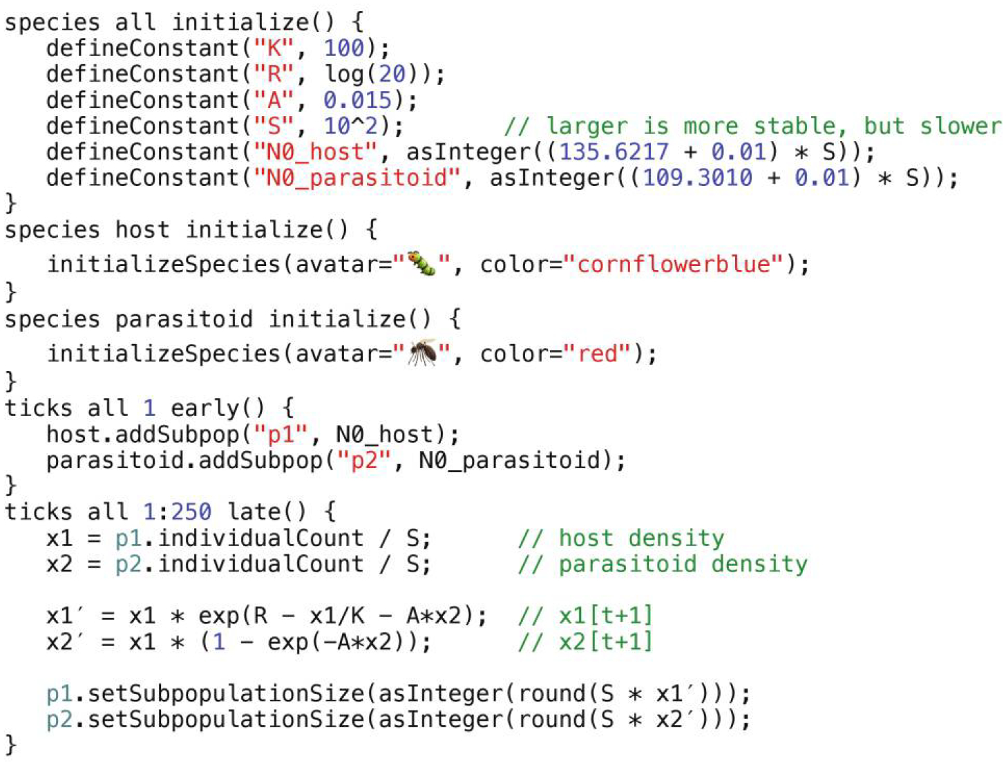
The “simple example” multispecies SLiM model.

Similarly, a review by Urban et al. (2021) reviewed 50 different modeling software packages (including SLiM 3) and found that overall, “current biodiversity models generally lack the biological realism, adaptability, interoperability, and integration needed to address the complexities of the biodiversity crisis” (p. 94). Figure 1 of Urban et al. (2021) shows a summary of their review; SLiM 3 suffers in their review particularly for its lack of support in areas such as species diversity, species interactions, biodiversity, and biomass. As they write, “We now find ourselves in the middle of the Anthropocene and ill equipped to predict and prevent biodiversity and ecosystem change” (p. 102).

We did a brief survey of the findings of Urban et al. (2021) to look for existing software packages that satisfied what we view as three key criteria for this area: (i) the software must provide support for genetics that allows evolution, (ii) the software must provide support for simulating multiple species, and (iii) the software must be individual-based (since models of multiple species with complex genetics are generally beyond the reach of analytical and coalescent approaches).

We found two software packages among those summarized in their review that satisfy those criteria. One is sPEGG (Okamoto and Amarasekare 2018), a C++ library that utilizes advanced GPU programming techniques such as THRUST and CUDA to provide extremely fast simulations. The other is HexSim (Schumaker and Brookes 2018), a Windows-based simulator that uses a hexagonal grid to represent space. We believe, however, that SLiM offers advantages over these packages, particularly in terms of the versatility of its genetics architecture, its overall scriptability and flexibility, and its ease of use. Finally, there are certainly many other very good forward genetic simulation software packages out there, such as fwdpp (Thornton 2014), Nemo (Guillaume and Rougemont 2006), MimicrEE2 (Vlachos and Kofler 2018), and SimBit (Matthey-Doret 2021). However, none of these provide intrinsic support for simulating multiple species as far as we are aware. In summary, as Urban et al. (2021) concluded, no existing software fulfils the important eco-evo-biodiversity modeling requirements they describe.

To fill this gap, we here announce the release of SLiM 4, a new major release of SLiM that adds extensive support for multispecies modeling. We will discuss the new additions to SLiM 4 that make multispecies modeling possible, and we will provide two example multispecies SLiM models for illustration.

Combined with the existing extensive and scriptable capabilities of SLiM, all of which can be used in multispecies SLiM 4 models, this represents a significant advance toward the “universal modeling platform” for biodiversity envisioned by Urban et al. (2021), although there is no doubt that much work still remains.

SLiM 4 Architecture

To introduce SLiM 4’s new multispecies capabilities we will need to get into some technical details, but we will try to illuminate the important concepts even if there are some aspects that are not completely clear for those who have never used SLiM. In SLiM 3, the top-level object class representing the entire single-species simulation, in the Eidos script that drives a SLiM simulation, is the class SLiMSim. The overall redesign strategy for SLiM 4 is to repurpose the SLiMSim class to represent a single species, as before, but now embedded in a multispecies context that is controlled by a new top-level class, the Community class. To better represent its new role, the SLiMSim class is renamed to Species. This redesign strategy is shown in figure 1.

Figure 1:

The architectural shift in SLiM to allow multispecies modeling. A, The architecture of SLiM 3, with a single SLiMSim object representing the entire simulation, comprising one species. Various aspects of the configuration of that single species are shown with shaded blocks, managed by the SLiMSim object. B, The new architecture of SLiM 4. The SLiMSim class has been renamed Species and represents one species in the simulation (as it did in SLiM 3). A new level in the object hierarchy, the Community class, has been added above the Species class, and can manage more than one Species.

This redesign strategy minimizes the complexity of the architectural change. Existing SLiM 3 models will continue to run in SLiM 4, with minor (if any) code changes, because the architecture of the two is so parallel. Multispecies models simply need to manage each species as a single-species SLiM 3 model would, with initialization and setup code, reproduction code, callbacks, output events, and so forth; such code just needs to exist for each species in the multispecies model. Finally, for situations where the species need to interact with each other or access global simulation state, the new top-level Community class ties everything together.

SLiM executes the “life cycle” of a simulated organism as a repeated sequence of stages like reproduction, fitness calculation, and mortality. In SLiM 3 this sequence was called the “generation cycle”; in SLiM 4 it is called the “tick cycle,” and each completed cycle is now called a “tick” instead of a “generation” for clarity (for details on this terminological shift, see box 2). The tick cycle executes for all active species, in an interleaved fashion; essentially, all species will reproduce (one immediately after the other), then all species will recalculate their fitness, then all species will undergo mortality, and so forth. A species might be inactive if it runs on a slower timescale than other species; in that case, it will not participate in the currently executing tick cycle. In a mosquito-human model, for example, mosquitoes might be active in every tick, while humans might be active only every tenth or hundredth tick. In many simple models, however, all of the species are active in every tick, and so the tick cycle executes simultaneously, in an interleaved fashion, for all of them.

Box 2: Time units in SLiM.

In SLiM 3 (and before), the term “generation” was used to refer to a single loop through SLiM’s life cycle stages, providing an opportunity for reproduction, event execution, fitness calculation, mortality, and so forth. Originally, when SLiM supported only Wright-Fisher models with nonoverlapping generations, this terminology made sense; one loop through those life cycle stages was, indeed, one generation. When SLiM 3 added non-Wright-Fisher models with overlapping generations and age structure, the term no longer fit well; one loop through those life cycle stages no longer necessarily had any relationship to biological generations at all. Now, with SLiM 4’s multispecies models, the term fits even less well because each species in a multispecies model might have a different life cycle with a different generation time.

To avoid further confusion, we have therefore abandoned the term “generation” in SLiM 4 and have instead introduced two new terms for specifying time: ticks and cycles. Ticks typically correspond to objective time; one tick might represent a day, a month, a season, a year, or any other fixed duration that you, the modeler, choose. Because ticks pass at the same rate for all species, the tick counter is managed by the Community object. By and large, the tick counter is the replacement for the generation counter of SLiM 3. Each species also has its own “cycle counter,” which represents time as observed by that species; in a model of mosquitoes and humans, for example, the mosquitoes might move and reproduce much more frequently than the humans do, so their cycle counter might advance more quickly than the human cycle counter does, but the tick counter kept by the global Community object is the same for all.

Some details of the multispecies architecture of SLiM 4 have been glossed over for brevity here; a complete description of the SLiM 4 rearchitecture is provided in the supplemental PDF. Rather than getting bogged down in those technical details, let us look at two example SLiM 4 multispecies models to see what all this looks like in practice.

A Simple Example

To illustrate the new capabilities outlined above, we will here look briefly at a simple example model (also shown in section 19.3 of the SLiM manual), based on a deterministic host-parasitoid model given in Faure and Schreiber (2014). The hosts are something like insects, perhaps caterpillars; they compete for food, and if they survive that competition then they reproduce by generating offspring, with some mean clutch size. The parasitoids are something like parasitoid wasps; they hunt the caterpillars and, when they find one, lay an egg. The egg, when it hatches, contains a larval wasp that will kill its host caterpillar and eventually turn into an adult wasp. Unlike the host, then, the parasitoids have no mean clutch size; instead, they generate one new offspring for each successful hunt. The deterministic model of Faure and Schreiber (2014) uses two iterative equations to calculate the population densities in the next generation for the host and parasitoid species, based on their population densities in the current generation:

$$x_1[t+1]=x_1[t]{\text{e}}^{r-x_1[t]/K-a{x}_2[t]}\text{, }$$

$$x_2[t+1]=x_1[t]\left(1-e^{-a{x}_2[t]}\right)\text{, }$$

where x₁ is the host density and x₂ is the parasitoid density, t is the time (in discrete time, not continuous time), and a, r, and K are free parameters (discussed more below, in the context of the SLiM model). The biological motivations for these equations are that (in sequential order) with probability 1 2 e^2ax2[t] each host is killed by a parasitoid, with probability e^2×1[t]=K each host then escapes death via competition, each surviving host produces a Poisson number of offspring with mean e^r, and all hosts killed by a parasitoid turn into a parasitoid in the next year. Faure and Schreiber (2014) provide further details; it is not really our focus here.

Instead, our focus is on the realization of this deterministic model in SLiM. Figure 2 shows the population dynamics of the implemented SLiM model. The abundance of the parasitoid tends to mirror that of the host, but with a lag of one or more ticks since high host abundance leads to a greater number of parasitoid offspring in the following tick. The dynamics are approximately cyclical, but the cycles are complex, even chaotic, because of the nature of the ecological interactions between the two species.

Figure 2:

Population size cycles in the host (blue) and parasitoid (red) species in the simple example model. Cycling begins slowly because the model starts near an equilibrium point.

This is a very trivial SLiM model, with no genetics, no individual-level behavior, and no population structure; it could be coded just as easily in Python, R, or any other programming language. The goal, with this first example model, is not to showcase SLiM’s capabilities; our second example model will begin to do that. Instead, the goal here is just to show a minimal multispecies model, to provide a first look at SLiM for those who have never used it before, and to show more experienced users the new multispecies extensions in SLiM 4.

The model, shown in figure 3, begins with three initialize() callbacks that initialize the simulation. The first, designated species all, initializes the overall model by setting up a few parameters: K, a scaling factor for the strength of competition between hosts; R, which scales the reproductive output of the host; A, which scales the probability that a host will be killed by a parasitoid; and S, which scales the size of the habitat and thus scales the population sizes attained by the model. It also calculates the initial population sizes for the host and parasitoid, which are slightly perturbed away from an equilibrium point of the model. The other two initialize() callbacks, designated species host and species parasitoid, declare the existence of these two species and configure them. Since this example model contains no genetics, the initialization code for them is very simple: we just set an “avatar” emoji and a color for each species, for the benefit of SLiMgui’s visualization of the model. As a result of these species declarations, global constants named host and parasitoid will exist in the simulation representing the two species (just as the global constant sim represents the single species in a SLiM 3 model).

After that is an early() event (an Eidos event that executes early in the tick cycle), declared to execute in tick 1, that creates initial subpopulations for each species, using the global host and parasitoid symbols to specify the species for each subpopulation. The addSubpop() method is called on each species to create the subpopulations, named p1 and p2. This event is designated with a ticks all prefix; this is a new SLiM 4 extension. The ticks all specifier tells SLiM that this event is not associated with any particular species, in terms of the timing of its execution; ticks host or ticks parasitoid would specify that the event ought to run only when that species is active, as mentioned earlier.

Finally, there is a late() event (an Eidos event that executes late in the tick cycle), declared to execute in every tick from 1 to 250, that implements the population dynamics of the model. It begins by calculating the current population density for each species (by dividing the population size by the habitat size S). It then uses the equations from Faure and Schreiber (2014), as shown above, to calculate the population densities for the two species in the next tick. (Note that Eidos allows a prime mark and other Unicode symbols like Greek letters and accented characters in variable names; x1′ and x2′ are simply variable names). At the end it sets the new population sizes for p1 and p2, obtained by multiplying the new population densities by the habitat size S.

That is the entirety of the model; its implementation is quite straightforward. We will look at a more interesting model next.

A Coevolutionary Example

As noted above, the first example model was quite trivial—really just a very fancy way of iterating the deterministic equations of the mathematical model. However, each individual in both species is actually created by SLiM as that model runs, and it would be a fairly small step to then add genetics to those individuals, make them interact with each other at an individual level in a way that depends on those genetics, and evolve in response to the selection pressures exerted by each other, producing coevolutionary dynamics. We will explore those possibilities now in our second example model.

This second model adds a quantitative phenotypic trait to both the host and the parasitoid species. You might think of the host phenotype as the scent of the host, perhaps a cuticular hydrocarbon signature or some such, and the parasitoid phenotype is the host scent that that parasitoid instinctively hunts, as coded by its genetics. If the phenotypic values of a particular host and parasitoid match, that parasitoid will be highly attracted by the scent of that host and thus more likely to find it, lay an egg in it, and kill it. Both of these phenotypic traits are based on the genetics of each individual, using a quantitative genetics type of approach: specific quantitative trait locus (QTL) mutations are simulated, each with a particular effect size drawn from an effect size distribution, and the phenotypic value of each individual is calculated from the additive effects of the mutations each individual possesses.

Furthermore, the hunting behavior of the parasitoids in this model is now simulated at the individual level and depends on the phenotypes of the parasitoids and the hosts. More specifically, this model simulates trait-based matching: each parasitoid preferentially hunts for hosts with a phenotypic value that is similar to the phenotypic value of the parasitoid itself. Both quantitative traits are under stabilizing selection; apart from that constraint, they are free to evolve in response to the ecology simulated by the model.

The resulting population dynamics from this SLiM model are shown in figure 4, both for a run with the trait-based matching in the hunting code turned off (fig. 4A) and for a run with that code enabled (fig. 4B). In the run without trait-based hunting (fig. 4A), the mean phenotypic value of each species essentially does a random walk around the stabilizing selection optimum and the evolutionary trajectories of the two species are uncorrelated. With trait-based matching (fig. 4B), however, the host evolves away from the parasitoid; more extreme phenotypic values decrease the probability of being killed. The parasitoid, however, evolves toward the host, chasing its phenotype. At a certain point, the host species runs into a wall due to the stabilizing selection in the model; it is so distant from the phenotypic optimum that evolving farther away from the parasitoid is not worth the price of the decrease in fitness due to stabilizing selection. The host is thus trapped between a rock and a hard place; but a few host individuals with extreme phenotypes exist on the opposite side of the parasitoid, and those hosts have the highest fitness. They survive while most of the other hosts get hunted, and so the host’s phenotypic mean actually jumps over that of the parasitoid and the host species begins to run away from the parasitoid species in the opposite direction. This pattern repeats cyclically, with some variations. These are so-called Red Queen coevolutionary dynamics (Van Valen 1973): the two species are both under continuous selective pressure to evolve, and yet, over time, they do not really get anywhere but merely cycle around an average phenotypic value.

Figure 4:

Evolutionary dynamics in the “coevolutionary example” multispecies SLiM model. The blue and red curves show the mean phenotype of the host and parasitoid, respectively, as a function of simulation time (tick). The shaded regions show 1 standard deviation around the mean. Note that the y-axis scales differ. A, The model with trait-based matching in the hunting code turned off (stabilizing selection is still enabled). B, The model with trait-based matching in the hunting code turned on.

The implementation of this model is shown in two parts in figures 5 and 6 (and is also presented in section 19.6 of the SLiM manual, in somewhat different form). The first part (fig. 5) begins again with initialize() callbacks. The species all initialize() callback sets up model parameters, as before; there are two new parameters, S_M and S_S, that we will see below. It also designates this model as a non-Wright-Fisher (nonWF) model; this will provide us with additional control over individual reproduction and mortality compared with the Wright-Fisher model type used in the first example.

Figure 5:

The “coevolutionary example” multispecies SLiM model (part I).

Figure 6:

The “coevolutionary example” multispecies SLiM model (part II).

The two species-specific initialize() callbacks now set up a genetic architecture for each species. It is essentially the same for both: a chromosome with discrete base positions from 0 to 9999, composed of a single “genomic element type” that undergoes mutations of a single “mutation type.” The mutation type models QTL mutations with additive effects upon a quantitative phenotypic trait in each species. The effect sizes for new QTL mutations are drawn from a normal distribution (type “n”) with a mean of 0.0 and a standard deviation of 0.1. Both species use a recombination rate of 10⁻⁸ and a mutation rate of 10⁻⁷ (per base position per tick). These parameters are somewhat arbitrarily chosen; we are not closely modeling any particular organism.

Next come two mutationEffect() callbacks. These essentially tell SLiM that all of the QTL mutations in this model (mutation types m1 and m2) should be treated by SLiM as neutral; we will handle the fitness effects due to these mutations ourselves, in script. This is because these mutations are not intrinsically beneficial or deleterious; instead, their effect on fitness will depend on the scripted interactions between the individuals in the two species.

Next, an early() event creates the two subpopulations p1 and p2 in tick 1, just as before.

Finally, this part of the model ends with an early() event that executes in every tick. This event begins by enforcing nonoverlapping generations to better match the Wright-Fisher dynamics of the first example model. To do this for the host species, it fetches a vector of all the host individuals into a variable named hosts, calls the killIndividuals() method to kill every host with an age greater than 0, and then narrows down the hosts variable to the survivors—new juveniles just created by reproduction. Nonoverlapping generations for the parasitoids is implemented identically, leaving us with a variable named parasitoids with the survivors.

This event then calculates phenotypic trait values for all surviving individuals and applies stabilizing selection to the individuals based on their phenotypes. All of this work is done with a series of vectorized operations, first for the hosts and then for the parasitoids: adding up the effect sizes of the QTL mutations possessed by each individual with sumOfMutationsOfType() to produce phenotypic values, looking up fitness values for those phenotypic values using dnorm() to implement a Gaussian fitness function, setting those fitness values into each individual’s fitnessScaling property, and remembering the phenotype for each individual in its tagF property. Vectorized operations like this are common in Eidos because they are highly efficient; a single Eidos statement can process a given step in these calculations across the whole vector of individuals in a species.

Note that the stabilizing fitness function provided by dnorm() has an optimum phenotypic value of 0.0 for both species in this model, and the further the phenotypic value of a given individual is from that optimum, the lower that individual’s fitness will be. The “width,” or standard deviation, of the Gaussian fitness function is controlled by the new parameter S_S, and the variable scale calculated beforehand is used to rescale the Gaussian fitness function to have a maximum value of exactly 1 at the fitness optimum. In nonWF models such as this, the default fitness implementation assumes absolute fitness with hard selection; if an individual’s fitness is, say, 0.6, that individual then has a 60% chance of surviving selection and a 40% chance of dying. The individual’s fitnessScaling property gets multiplied together with any other fitness effects in the model (in this model there are no others) to produce a final fitness value for the individual; setting fitnessScaling thus sets up the probability that each individual will survive stabilizing selection according to the fitness value provided by dnorm().

The second part of this model, shown in figure 6, begins with a first() event (executed first thing in each tick) that will run in every tick from 2 to 10000. (It starts in tick 2 because the subpopulations for the two species do not yet exist at that point in tick 1—they are created in an early() event in tick 1, as we saw above, which executes after first() events.) This first() event is really the core of the logic of the model; it handles the hunting of the hosts by the parasitoids, as well as the competition among the surviving hosts. It is fairly complex; we will go through it part by part beginning at the top, where the host and parasitoid individuals are fetched from the species objects and the density of each species is calculated by dividing by the habitat size S as before.

Next we assess the match between the phenotypes of the hosts and the phenotypes of the parasitoids. The appeal of a given host to the hunting parasitoids can be approximated by the match between the phenotype of the host and the mean phenotype of all of the parasitoids; to do this, we first calculate the mean parasitoid phenotype, and we then compare each host’s phenotype to that mean. To make that comparison we use dnorm() to implement a Gaussian trait-matching function, this time with a width of S_M, again rescaling to a maximum of 1 for a perfect match.

Next, armed with the vector host_match that contains the degree of match between each host and the mean parasitoid, we can conduct the hunt. Each parasitoid keeps track of the number of eggs it has laid in its tag property; like tagF above (where we stored individual phenotype values), this is a general-purpose property that we are free to use for whatever purpose we wish. We zero out the tag values for all parasitoids at the start of the hunt. Then we do a vectorized calculation to obtain the probability that each host will be hunted and killed, based on its match to the mean parasitoid; this is essentially one of the terms in the original mathematical model, scaled by the degree of the phenotypic match for each host. Given this vector of probabilities (one per host), we do a binomial draw for each host to see whether it does get hunted and killed, producing a vector named dead that contains all of the hosts slated for death. Next we need to determine which parasitoid hunted each killed host; this is done with a call to sapply() that does a weighted draw of a parasitoid for each killed host. The weights for the draw are the match between each parasitoid and the host in question, from the same Gaussian trait-matching function as before, implemented again with dnorm() using the width S_M. (Note that the syntax for the sapply() function is a bit odd because it takes executable code, executed for every individual in dead, as a string value; in its effect it is much like a for loop run over the elements of dead.) Having determined which parasitoids got each kill, a for loop increments the parasitoid tag values for each successful kill; at the end of this loop, the tag value of each parasitoid is equal to its total number of kills. Finally, we actually kill the hosts that were hunted, by passing dead to killIndividuals().

The last part of the first() event handles densitydependent competition among the surviving hosts. This is essentially the same, mechanistically, as the corresponding term in the mathematical model, but it is individual-based. As in the hunt code, we use rbinom() to do a binomial draw for each individual host, determining which specific individuals live and die. We use the killIndividuals() method again to kill the hosts that did not survive competition, as we did for hunting.

The reproduction() callbacks in figure 6 are called by SLiM for each living individual in the model, at the point in the tick cycle when reproduction occurs, as in SLiM 3. Each time one of these callbacks is called, there is a specific focal individual that is expected to reproduce itself, provided by SLiM in the local variable individual, which lives in the subpopulation named subpop. The code first determines the litter size to generate—for the hosts with a Poisson draw with mean e^r (as in the mathematical model) and for the parasitoids using the number of kills that individual got (as recorded in the parasitoid’s tag property). We then choose a mate with sampleIndividuals() and generate new offspring up to the calculated litter size with that mate by calling the addCrossed() method in a for loop. This is fairly typical reproduction code for a SLiM nonWF model. Notice, however, that these callbacks are declared with species host and species parasitoid prefixes, just as the species-specific initialize() callbacks were, to tell SLiM which species each reproduction() callback applies to.

That is the entirety of the second model. It is, in some sense, two separate SLiM 3 models, one for each species; the two species have separate initialization code and separate reproduction code, live in different subpopulations, and have very different behaviors. However, they are specified in a single script, and their life cycles execute simultaneously, in an interleaved fashion. They interact with each other, and their survival and reproduction depends on the outcome of that interaction. This model is a bit complex to explain line by line, but in about two pages of code we have constructed a two-species model of coevolutionary dynamics, underpinned by explicitly modeled QTL mutations that additively influence quantitative phenotypic traits in the two species. SLiM handles all of the details of the genetics for us, including new mutation generation, recombination, and linkage between QTLs; a great deal goes on under the covers with each call to addCrossed().

This model could be extended in many ways. The individuals could live on a continuous spatial landscape, for example, with spatial variation in the stabilizing selection optima. The species could possess multiple phenotypic traits influenced (pleiotropically or not) by the mutations in the model, affecting behaviors besides hunting, such as dispersal propensity or fecundity. Other species—perhaps a plant species for the hosts to eat?—could be added, perhaps introducing more complex trophic effects that would cascade through the food web. Temporal change could occur in the spatial landscape and other parameters, perhaps due to climate change. Many other ideas are possible too; because SLiM is scriptable, you can construct more or less whatever evolutionary model you wish.

Discussion

SLiM 4 extends the existing SLiM forward genetic simulation framework, adding the capability of modeling multiple species and the ecological interactions between them. This moves SLiM much closer to the universal modeling platform that Urban et al. (2021) make clear is needed for evolutionary ecology and biodiversity studies.

There are a few changes in SLiM 4 that we have not explored here, for reasons of brevity. One is extensions to SLiMgui, SLiM’s graphical modeling environment, to support multispecies models. Suffice to say that it now displays the state of each simulated species (or all together, in a unified view), it can graph results from each species separately (or, in some cases, show results from multiple species in a single plot), it can annotate the display of the SLiM script to indicate which species each code block is associated with, and so forth, providing a high level of integration between the scripting environment and the model.

Another is extensions to InteractionType, the class used in SLiM to find and evaluate interactions between individuals (particularly local interactions in continuous-space models). InteractionType now supports interspecies interactions, in addition to the intraspecies interactions supported in SLiM 3. To achieve this, a fundamental redesign of InteractionType was needed under the hood; however, the calling interface for it is almost completely unchanged, and it is actually more efficient, particularly in its memory usage, than it was in SLiM 3.

A third change involves tree-sequence recording, the recording of true local genetic ancestry information along the genome for individuals in a SLiM model. In a multispecies tree-sequence model, each species has its own separate recorded tree sequence. In most respects this works as it did in SLiM 3, but some changes, such as the shift from “generations” to ticks and cycles, necessitated minor changes to the tree-sequence metadata annotations used by SLiM. Corresponding changes were made to the pyslim package; pyslim version 1.0 or later should therefore be used with SLiM 4 for correct functioning and can be installed with pip. Documentation for pyslim is at https://tskit.dev/pyslim/docs, and an overview of what changed and how to update your pyslim code is at https://tskit.dev/pyslim/docs/latest/previous_versions.html.

There are areas pointed out by Urban et al. (2021) where further additions to SLiM might make biodiversity modeling easier, such as support for modeling physiology and functional groups (although SLiM’s scriptability may be the best way to approach some such problems). We plan to address such limitations in future versions of SLiM, which remains under very active development. We also welcome feedback from users, including feature requests, and we would be particularly interested to hear from researchers who are trying out the new multispecies features of SLiM 4.

We are very excited by what SLiM 4 can do, and we believe that its new features will broaden its utility beyond population genetics into eco-evolutionary and ecological modeling, biodiversity modeling, and conservation and management applications.

Data and Code Availability

SLiM is open source on GitHub (https://github.com/MesserLab/SLiM). An archive of the source code and manuals for SLiM version 4.0.1 is available on Zenodo (https://doi.org/10.5281/zenodo.7331688; Haller and Messer 2022).

Literature Cited

- Baumdicker F, Bisschop G, Goldstein D, Gower G, Ragsdale AP, Tsambos G, Zhu S, et al. 2022. Efficient ancestry and mutation simulation with msprime 1.0. Genetics 220:iyab229. [DOI] [PMC free article] [PubMed] [Google Scholar]
- Faure M, and Schreiber SJ. 2014. Quasi-stationary distributions for randomly perturbed dynamical systems. Annals of Applied Probability 24:553–598. [Google Scholar]
- Guillaume F, and Rougemont J. 2006. Nemo: an evolutionary and population genetics programming framework. Bioinformatics 22:2556–2557. [DOI] [PubMed] [Google Scholar]
- Haller BC, Galloway J, Kelleher J, Messer PW, and Ralph PL. 2019. Tree-sequence recording in SLiM opens new horizons for forward-time simulation of whole genomes. Molecular Ecology Resources 19:552–566. [DOI] [PMC free article] [PubMed] [Google Scholar]
- Haller BC, and Messer PW. 2017. SLiM 2: flexible, interactive forward genetic simulations. Molecular Biology and Evolution 34:230–240. [DOI] [PubMed] [Google Scholar]
- ———. 2019a. Evolutionary modeling in SLiM 3 for beginners. Molecular Biology and Evolution 36:1101–1109. [DOI] [PMC free article] [PubMed] [Google Scholar]
- ———. 2019b. SLiM 3: forward genetic simulations beyond the Wright–Fisher model. Molecular Biology and Evolution 36:632–637. [DOI] [PMC free article] [PubMed] [Google Scholar]
- ———. 2022. SLiM version 4.0.1. American Naturalist. 10.5281/zenodo.7331688. [DOI] [Google Scholar]
- Matthey-Doret R 2021. SimBit: a high performance, flexible and easy-to-use population genetic simulator. Molecular Ecology Resources 21:1745–1754. [DOI] [PubMed] [Google Scholar]
- Messer PW 2013. SLiM: simulating evolution with selection and linkage. Genetics 194:1037–1039. [DOI] [PMC free article] [PubMed] [Google Scholar]
- Okamoto KW, and Amarasekare P. 2018. A framework for high-throughput eco-evolutionary simulations integrating multilocus forward-time population genetics and community ecology. Methods in Ecology and Evolution 9:525–534. [Google Scholar]
- Ralph PL, Thornton K, and Kelleher J. 2020. Efficiently summarizing relationships in large samples: a general duality between statistics of genealogies and genomes. Genetics 215:779–797. [DOI] [PMC free article] [PubMed] [Google Scholar]
- Schumaker NH, and Brookes A. 2018. HexSim: a modeling environment for ecology and conservation. Landscape Ecology 33:197–211. [DOI] [PMC free article] [PubMed] [Google Scholar]
- Thornton KR 2014. A C11 template library for efficient forward-time population genetic simulation of large populations. Genetics 198:157–166. [DOI] [PMC free article] [PubMed] [Google Scholar]
- Urban MC, Travis JMJ, Zurell D, Thompson PL, Synes NW, Scarpa A, Peres-Neto PR, et al. 2021. Coding for life: designing a platform for projecting and protecting global diversity. BioScience 72:91–104. [Google Scholar]
- Van Valen L 1973. A new evolutionary law. Evolutionary Theory 1:1–30. [Google Scholar]
- Vlachos C, and Kofler R. 2018. MimicrEE2: genome-wide forward simulations of evolve and resequencing studies. PLoS Computational Biology 14:e1006413. [DOI] [PMC free article] [PubMed] [Google Scholar]
- Zurell D, König C, Malchow A-K, Kapitza S, Bocedi G, Travis J, and Fandos G. 2022. Spatially explicit models for decisionmaking in animal conservation and restoration. Ecography 2022: e05787. [Google Scholar]
Associated Data
This section collects any data citations, data availability statements, or supplementary materials included in this article.
Data Availability Statement