Review of machine learning and deep learning models for toxicity prediction

Wenjing Guo; Jie Liu; Fan Dong; Meng Song; Zoe Li; Md Kamrul Hasan Khan; Tucker A Patterson; Huixiao Hong

doi:10.1177/15353702231209421

. 2023 Dec 6;248(21):1952–1973. doi: 10.1177/15353702231209421

Review of machine learning and deep learning models for toxicity prediction

Wenjing Guo ¹, Jie Liu ¹, Fan Dong ¹, Meng Song ¹, Zoe Li ¹, Md Kamrul Hasan Khan ¹, Tucker A Patterson ¹, Huixiao Hong ^1,^✉

PMCID: PMC10798180 PMID: 38057999

Abstract

The ever-increasing number of chemicals has raised public concerns due to their adverse effects on human health and the environment. To protect public health and the environment, it is critical to assess the toxicity of these chemicals. Traditional in vitro and in vivo toxicity assays are complicated, costly, and time-consuming and may face ethical issues. These constraints raise the need for alternative methods for assessing the toxicity of chemicals. Recently, due to the advancement of machine learning algorithms and the increase in computational power, many toxicity prediction models have been developed using various machine learning and deep learning algorithms such as support vector machine, random forest, k-nearest neighbors, ensemble learning, and deep neural network. This review summarizes the machine learning- and deep learning-based toxicity prediction models developed in recent years. Support vector machine and random forest are the most popular machine learning algorithms, and hepatotoxicity, cardiotoxicity, and carcinogenicity are the frequently modeled toxicity endpoints in predictive toxicology. It is known that datasets impact model performance. The quality of datasets used in the development of toxicity prediction models using machine learning and deep learning is vital to the performance of the developed models. The different toxicity assignments for the same chemicals among different datasets of the same type of toxicity have been observed, indicating benchmarking datasets is needed for developing reliable toxicity prediction models using machine learning and deep learning algorithms. This review provides insights into current machine learning models in predictive toxicology, which are expected to promote the development and application of toxicity prediction models in the future.

Keywords: Toxicity, machine learning, deep learning, model, dataset, data quality

Impact Statement

Machine learning- and deep learning-based toxicity prediction models have become popular due to their ability to predict the toxicity of chemicals accurately and economically. There is not a comprehensive review that summarizes current developments and applications of machine learning and deep learning models for predicting various toxicity endpoints and discusses factors impacting model performance, especially the quality of datasets. This review aims to fill this cap by discussing the current machine learning and deep learning models to aid the development of more reliable toxicity prediction models using machine learning. We examine current machine learning and deep learning models for toxicity prediction from common toxicities, machine learning algorithms, and datasets. We also discuss the efforts that are crucial to improving the performance of toxicity prediction models in the future.

Introduction

The safety of chemical-containing products and the risks of environmental chemicals have become one of the most serious problems for people all over the world due to the ever-increasing number of chemicals. To reduce the potential adverse effects of chemicals on human health, it is crucial to assess the toxic effects associated with exposure to chemicals. Toxicity assessments have been used by regulatory decision-making bodies such as the U.S. Food and Drug Administration (FDA), U.S. Environmental Protection Agency (EPA), European Environment Agency, and European Medicines Agency (EMA) to ensure public safety by reducing human and environmental exposure to harmful chemicals. Currently, the standard methods of toxicity evaluation are based on animal experiments. However, these tests are constrained by time, cost, and ethical issues. Moreover, it is impossible to test such a large number of compounds for toxicological, regulatory, or drug development purposes via animal experimentation. To address these challenges, it is crucial to develop fast and economical alternatives to avoid conducting animal toxicity tests, including in vitro and in silico methods.

In recent decades, various computational methods such as structural alerts, read-across, and quantitative structure-activity relationship (QSAR) have been used to predict the toxicological effects of chemicals.^1–14 QSAR builds a quantitative relationship between the structural or physicochemical characteristics of chemicals and their toxic effects. It has been one of the widely used methods to build toxicity prediction models. Recently, due to the continuous improvement of computational power, the emergence of big data, and the rapid development of machine learning (ML) and deep learning (DL) techniques, QSAR based on ML and DL has become increasingly prominent in predictive toxicology. The ability to automatically learn from data to perform predictions makes ML and DL very attractive computational techniques to predict toxicity for a large number of chemicals. Our group has used ML to estimate various physicochemical properties and toxicological activities of chemicals.^{1,2,4,6,8,9,15,16}

Although enormous progress has been made in implementing ML- and DL-based models in predictive toxicology, there are growing interests in developing more reliable toxicity prediction models using ML and DL. A comprehensive review to summarize the current development and applications of ML and DL models in predictive toxicology may provide insight and promote and improve the development of more reliable ML and DL models in predictive toxicology. This review recapitulates current ML and DL models in predictive toxicology and discusses various factors related to the models and their performance.

Toxicity types

Many ML and DL models have been built to predict a variety of toxicity types. In Table 1, ML algorithms and their performance were analyzed for models from 82 papers. For paper selection, we conducted searches on PubMed (https://pubmed.ncbi.nlm.nih.gov/) using a combination of keywords including (“toxicity” or “carcinogenicity” or “cardiotoxicity” or “cytotoxicity” or “genotoxicity” or “hepatoxicity” or “acute toxicity” or “skin toxicity” or “reprotoxicity”) and (“machine learning” or “deep learning”). To ensure the reports are current, we only considered papers published after 2008. Furthermore, we focused on papers with classification models that reported balanced accuracy in their cross validation (on the entire dataset, not just the training dataset), holdout, and external validation. From this analysis, we summarized a total of 82 papers, specifically addressing models for predicting carcinogenicity, cardiotoxicity, cytotoxicity, genotoxicity, hepatoxicity, acute toxicity, skin toxicity, and reprotoxicity. This review intentionally excludes models geared toward predicting other types of toxicity to maintain a focused scope. The balanced accuracy values for cross validation, holdout validation, and external validation are given in this table. For some external validations, the external dataset was obtained by splitting the same dataset into training and external datasets, and we listed them as holdout validations in the table. For models without balanced accuracy reported, the reported sensitivity and specificity were used to calculate balance accuracy.

Table 1.

Summary of machine learning and deep learning models for toxicity prediction.

Toxicity type	Dataset		Algorithm	Descriptors	Feature selection	Model validation			Ref
Toxicity type	Endpoint	Size	Algorithm	Descriptors	Feature selection	CV	Holdout	External	Ref
Carcinogenicity	In vivo (dog)	25	RF	MOE, MACCS	SW, PCA1	0.72	0.7		⁵⁹
	In vivo (hamster)	72	RF	MOE, MACCS	SW, PCA1	0.72	0.54		⁵⁹
	In vivo (rat)	829	DT	PaDEL	NS		0.697^a		⁶⁷
		829	kNN	PaDEL	NS		0.806^a	0.700 ^a	⁶⁷
		829	NB	PaDEL	NS		0.640^a		⁶⁷
		829	RF	PaDEL	NS		0.734^a	0.724	⁶⁷
		829	SVM	PaDEL	NS		0.802^a	0.692 ^a	⁶⁷
		852	SVM	MOE, MACCS	SW, PCA2	0.738^a	0.825^a		⁶⁶
		897	RF	MOE, MACCS	SW, PCA1	0.64	0.665		⁵⁹
		1003	CNN	Multiple₁	NA	0.663^a		0.679^a	⁶⁴
		1003	EL^b	PaDEL	PCA2	0.676^a		0.665	⁶⁵
		1003	EL^c	PaDEL	PCA2	0.670^a		0.687	⁶⁵
		1003	EL^d	PaDEL	PCA2	0.682^a		0.709	⁶⁵
		1003	kNN	Multiple₁	NA	0.599^a		0.648^a	⁶⁴
		1003	RF	PaDEL	PCA2	0.647^a			⁶⁵
		1003	RF	Multiple₁	NA	0.656^a		0.663^a	⁶⁴
		1003	SVM	PaDEL	PCA2	0.638^a			⁶⁵
		1003	SVM	Multiple₁	NA	0.618^a		0.701^a	⁶⁴
		1003	XGBoost	PaDEL	PCA2	0.647^a			⁶⁵
		1003	XGBoost	Multiple₁	NA	0.641^a		0.609^a	⁶⁴
		1042	NB	Multiple₂	NS	0.643^a			⁶³
		844	MLP	Multiple₃	PCA2, F-score, MC-SA		0.824		⁷⁰
		844	SVM	Multiple₃	PCA2, F-score, MC-SA		0.834		⁷⁰
		854	RF	PaDEL	CAS	0.782		0.58	⁶¹
		374	RF	PaDEL	CAS	0.6			⁶¹
	In vivo	172	SVM	SMILES	NS	0.909^a	0.904		⁶⁹
		665	SVM	SMILES	NS	0.756^a	0.76		⁶⁹
	Multicell	818	RF	MOE, MACCS	SW, PCA1	0.685	0.685		⁵⁹
	Single-cell	1121	RF	MOE, MACCS	SW, PCA1	0.625	0.665		⁵⁹
	In vivo (mouse)	1391	RF	MACCS, Morgan	NS	0.812		0.833	³⁰
	In vivo (rat and mice)	314	kNN	MCZ	NS		0.675^a		⁶²
		384	kNN	MCZ	NS		0.764^a	0.615	⁶²
Cardiotoxicity	IC50 (hERG)	172	EL^e	PaDEL	NA	0.703^a		0.578^a	⁵¹
		172	kNN	PaDEL	NA	0.656^a		0.556^a	⁵¹
		368	RF	Multiple₄	NS			0.745^a	⁴⁵
		368	SVM	Multiple₄	NS			0.77^a	⁴⁵
		476	RF	Multiple₄	NS			0.49^a	⁴⁵
		476	SVM	Multiple₄	NS			0.63^a	⁴⁵
		620	Bayesian	Multiple₅	NS	0.828^a			⁴⁴
		620	RP	ECFP_8	NS	0.845^a			⁴⁴
		697	MLP	Multiple₆	LV, HC		0.775^a	0.556^a	⁴⁹
		697	RF	Multiple₆	LV, HC		0.782^a	0.546^a	⁴⁹
		740	Bayesian	Multiple₅	NS		0.852^a	0.658^a	⁴⁴
		740	RP	ECFP_8	NS		0.805^a		⁴⁴
		1163	DT	Multiple₇	NS	0.664^a			⁵⁴
		1163	kNN	Multiple₇	NS	0.700^a		0.612^a	⁵⁴
		1163	NB	Multiple₇	NS	0.649^a			⁵⁴
		1163	RF	Multiple₇	NS	0.641^a			⁵⁴
		1163	SVM	Multiple₇	NS	0.701^a		0.597^a	⁵⁴
		1668	SVM	Multiple₈	NS	0.912^a		0.706^a	⁴⁶
		1865	EL^f	PaDEL	LV, HC	0.726^a		0.68	⁵⁰
		1865	RF	PaDEL	LV, HC	0.693^a			⁵⁰
		1865	SVM	PaDEL	LV, HC	0.690^a			⁵⁰
		1865	XGBoost	PaDEL	LV, HC	0.712^a			⁵⁰
		1939	ASNN	Multiple₉	PW	0.846^a		0.783^a	⁴⁸
		1939	kNN	Multiple₉	PW	0.838^a		0.735^a	⁴⁸
		1939	SVM	Multiple₉	PW	0.853^a		0.770^a	⁴⁸
		1939	RF	Multiple₉	PW	0.836^a		0.753^a	⁴⁸
		2117	kNN	Multiple₄	NS	0.58^a			⁴⁵
		2117	RF	Multiple₄	NS	0.515^a			⁴⁵
		2117	SVM	Multiple₄	NS	0.505^a			⁴⁵
		2130	LR	DRAGON, ECFP	HC	0.701			⁴⁷
		2130	MLP	DRAGON, ECFP	HC	0.644			⁴⁷
		2130	RR	DRAGON, ECFP	HC	0.68			⁴⁷
		2217	kNN	Multiple₄	NS	0.77^a			⁴⁵
		2217	RF	Multiple₄	NS	0.675^a			⁴⁵
		2217	SVM	Multiple₄	NS	0.66			⁴⁵
		2317	kNN	Multiple₄	NS	0.855^a			⁴⁵
		2317	RF	Multiple₄	NS	0.815^a			⁴⁵
		2317	SVM	Multiple₄	NS	0.78			⁴⁵
		2389	Bayesian	PC	NS		0.83	0.625	⁵⁵
		2389	Bayesian	PC, ECFP_14	NS		0.91	0.59	⁵⁵
		2389	RF	Multiple₄	NS			0.89	⁴⁵
		2389	SVM	Multiple₄	NS			0.83	⁴⁵
		2660	GCN	MG	NA		0.863		⁵²
		2660	SVM	Morgan	LV, HC, RFE		0.837		⁵²
		3024	RF	Multiple₄	NS			0.76^a	⁴⁵
		3024	SVM	Multiple₄	NS			0.75^a	⁴⁵
		3223	kNN	Multiple₄	NS	0.848^a			⁴⁵
		3223	RF	Multiple₄	NS	0.865^a		0.789^a	⁴⁵
		3223	SVM	Multiple₄	NS	0.79^a		0.748^a	⁴⁵
		3591	RF	Multiple₄	NS			0.765^a	⁴⁵
		3591	SVM	Multiple₄	NS			0.75^a	⁴⁵
		3634	GCN	MG	NA		0.81		⁵²
		3634	SVM	MD	NA		0.809		⁵²
		3699	RF	Multiple₄	NS			0.84^a	⁴⁵
		3699	SVM	Multiple₄	NS			0.785^a	⁴⁵
		3721	ASNN^g1	Multiple₉	PW	0.743^a		0.770^a	⁴⁸
		3721	ASNN^g2	Multiple₉	PW	0.727^a		0.742^a	⁴⁸
		3721	EL^g1h	Multiple₉	PW	0.757^a		0.776^a	⁴⁸
		3721	kNN^g1	Multiple₉	PW	0.718^a		0.629^a	⁴⁸
		3721	kNN^g2	Multiple₉	PW	0.674		0.678	⁴⁸
		3721	SVM^g1	Multiple₉	PW	0.714^a		0.736^a	⁴⁸
		3721	SVM^g2	Multiple₉	PW	0.722^a		0.737^a	⁴⁸
		3721	RF^g1	Multiple₉	PW	0.687^a		0.690^a	⁴⁸
		3721	RF^g2	Multiple₉	PW	0.704^a		0.716^a	⁴⁸
		4556	GCN	MG	NA		0.756		⁵²
		4556	GCN	MG	NA		0.802		⁵²
		4556	GCN	MG	NA		0.778		⁵²
		4556	RF	Morgan	LV, HC, RFE		0.734		⁵²
		4556	RF	Morgan	LV, HC, RFE		0.743		⁵²
		4556	SVM	Morgan	LV, HC, RFE		0.755		⁵²
		5612	RF	Multiple₄	NS			0.91^a	⁴⁵
		5612	SVM	Multiple₄	NS			0.86^a	⁴⁵
		5804	kNN^g1	Multiple₄	NS	0.74^a			⁴⁵
		5804	kNN^g2	Multiple₄	NS	0.715^a			⁴⁵
		5804	RF^g1	Multiple₄	NS	0.718^a			⁴⁵
		5804	RF^g2	Multiple₄	NS	0.72^a			⁴⁵
		5804	SVM^g1	Multiple₄	NS	0.623^a			⁴⁵
		5804	SVM^g2	Multiple₄	NS	0.633^a			⁴⁵
		5984	EL^b	Multiple₁₀	HC		0.798^a		²⁸
		5984	NN-MDRA	Multiple₁₀	HC		0.765^a		²⁸
		6247	RF	Multiple₄	NS			0.82^a	⁴⁵
		6247	SVM	Multiple₄	NS			0.80^a	⁴⁵
		7889	MLP	Mol2vec, MOE	NS		0.873^a		⁴²
		12,620	MLP	Multiple₁₁	NS	0.843^a			¹²²
		12,620	GCNN	Multiple₁₁	NS	0.81			¹²²
		12,620	CNN	Multiple₁₁	NS	0.818^a			¹²²
		12,620	EL^t	Multiple₁₁	NS	0.847^a		0.770^a	¹²²
		14,440	MLP	Multiple₁₂	NA	0.822^a	0.830^a		⁴³
		14,440	DLⁱ	Multiple₁₃	NA		0.811	0.738	⁴³
		14,440	GCNN	MG	NA	0.8	0.797		⁴³
Cytotoxicity	Human cell line	50	SVM	Multiple₁₄	NS			0.536^a	⁸²
		547	RF	PC	NS		0.782		⁸¹
		651	RF	PC	NS		0.761		⁸¹
		965	RF	PC	NS		0.854		⁸¹
		1099	RF	PC	NS		0.862		⁸¹
		1244	RF	PC	NS		0.809	0.692	⁸¹
		1300	RF	Multiple₁₄	NS			0.521^a	⁸²
		1300	SVM	Multiple₁₄	NS			0.529^a	⁸²
		1659	RF	PC	NS		0.808		⁸¹
		1685	RF	PC	NS		0.767		⁸¹
		2041	RF	PC	NS		0.796		⁸¹
		2258	RF	PC	NS		0.826		⁸¹
		3316	EL^b	Multiple₁₅	LV, HC	0.725^a	0.67		⁸⁴
		3316	RF	Multiple₁₅	LV, HC	0.582^a			⁸⁴
		5201	RF	PC	NS		0.783		⁸¹
		5429	RF	PC	NS		0.8		⁸¹
		5487	RF	MACCS, Morgan	NS	0.85		0.836	³⁰
		5784	RF	ECFP_4	NS			0.775^a	⁸⁵
		8833	RF	PC	NS		0.783		⁸¹
		27,492	MLP	Morgan	5-time	0.689			⁸³
		27,492	RF	Morgan	5-time	0.683			⁸³
		41,198	EL^b	Multiple₁₅	LV, HC	0.704			⁸⁴
		52,513	EL^b	Multiple₁₅	LV, HC	0.746			⁸⁴
		62,655	EL^b	Multiple₁₅	LV, HC	0.74			⁷⁸
	Mouse cell line	338	RF	PC	NS		0.83		⁸¹
		378	RF	PC	NS		0.605		⁸¹
		4080	RF	PC	NS		0.759		⁸¹
		12,388	EL^b	Multiple₁₅	LV, HC	0.856			⁸⁴
	Rat cell line	3727	RF	PC	NS		0.783		⁸¹
Genotoxicity	Combined^r	230	DF	PC, OFG	NS	0.989			⁹²
		230	DT	PC, OFG	NS	0.652^a			⁹²
	Comet assay	49	DT	MLB	NS		0.75		⁹⁴
	GreenScreen assay	1415	RF	PaDEL	CAS	0.908		0.541	⁵⁵
	In vivo micronucleus assay	641	MLP	Multiple₁₆	LV, HC, RFE	0.841^a	0.906^a		⁹³
		641	DT	Multiple₁₆	LV, HC, RFE	0.810^a			⁹³
		641	kNN	Multiple₁₆	LV, HC, RFE	0.806^a			⁹³
		641	NB	Multiple₁₆	LV, HC, RFE	0.819^a	0.86		⁹³
		641	RF	Multiple₁₆	LV, HC, RFE	0.817^a	0.937		⁹³
		641	SVM	Multiple₁₆	LV, HC, RFE	0.863^a	0.877^a		⁹³
	Mammalian cells	85	MLP	PC, OFG	NS			0.915	⁹²
		85	EL^j	PC, OFG	NS			0.927	⁹²
		85	LR	PC, OFG	NS			0.902	⁹²
		85	RF	PC, OFG	NS			0.816	⁹²
	Ames assay	49	DT	MLB	NS		0.83		⁹⁴
		658	RF	MOE, MACCS	PCA1, SW	0.74	0.715		⁵⁹
		2262	MLP	DRAGON, TSAR	SFFS, HC		0.607		⁷⁸
		2262	Bayesian	DRAGON, TSAR	SFFS, HC		0.67		⁷⁸
		2262	SVM	DRAGON, TSAR	SFFS, HC		0.717		⁷⁸
		4361	EL^b	Multiple₉	HC			0.788^a	²⁸
		4361	NN-MDRA	Multiple₉	HC			0.793^a	²⁸
		6156	RF	MACCS, Morgan	NS	0.84		0.85	³⁰
		6307	GCNN	MG	NA	0.805^a		0.759^a	⁷⁷
		6448	NB	Multiple₁₇	NS	0.694^a		0.624^a	⁷⁶
		6448	RP	Multiple₁₈	NS	0.757		0.653	⁷⁶
		6509	MLP	Multiple₁₉	NS	0.715^a			⁷⁵
		6509	Light GBM	Multiple₁₉	NS	0.793^a			⁷⁵
		6509	RF	Multiple₁₉	NS	0.726^a			⁷⁵
		6509	SVM	Multiple₁₉	NS	0.779^a			⁷⁵
		6509	XGBoost	Multiple₁₉	NS	0.776^a			⁷⁵
		6512	AdaBoost	Multiple₂₀	NA		0.788^a		⁷⁴
		6512	DT	Multiple₂₀	NA		0.767		⁷⁴
		6512	EL^k	Multiple₂₀	NA		0.801 ^a		⁷⁴
		6512	EL^e	Multiple₂₀	NA		0.746^a		⁷⁴
		6512	EL^c	Multiple₂₀	NA		0.813^a		⁷⁴
		6512	kNN	Multiple₂₀	NA		0.779		⁷⁴
		6512	RF	PaDEL	CAS	0.815		0.532	⁵⁵
		6512	SVM	Multiple₂₀	NA		0.797		⁷⁴
		8348	MLP	PaDEL	NS	0.795			⁷³
		18,947	MLP	ECFP	LRFS		0.875		⁷²
		18,947	LR	ECFP	LRFS		0.878		⁷²
		18,947	LSTM	ECFP	LRFS		0.873^a		⁷²
Hepatotoxicity	DILI	96	Bayesian^l1	ECPF6	NS	0.702		0.586^a	²⁴
		96	Bayesian^l2	ECPF6	NS	0.636		0.589^a	²⁴
		102	EL^b	Multiple₉	HC			0.490^a	²⁸
		102	NN-MDRA	Multiple₉	HC			0.509^a	²⁸
		116	SVM	Toxicogenomics	NS	0.731^a			²⁷
		221	Bayesian^l3	ECPF6	NS	0.733		0.614^a	²⁴
		221	Bayesian ^l4	ECPF6	NS	0.716		0.615^a	²⁴
		221	Bayesian ^l5	ECPF6	NS	0.718		0.660^a	²⁴
		221	Bayesian ^l6	ECPF6	NS	0.793		0.603^a	²⁴
		312	RF	PaDEL	NS			0.574^a	¹¹⁷
		312	SVM	PaDEL	NS			0.575^a	¹¹⁷
		387	DF	Mold2	CR1	0.69		0.632 ^a	¹³⁸
		401	RF	ECFP4	NS	0.734	0.741^a	0.583^a	³²
		401	SVM	ECFP5	NS	0.714	0.736^a	0.598^a	³²
		451	DF	Mold2	CR2	0.713			¹
		617	EL^m	Multiple₂₁	CR3		0.65^a		²⁹
		617	GLM	CCR	HC		0.56^a		²⁹
		617	MLP	Multiple₂₂	HC		0.59^a		²⁹
		617	QDA	CCR	HC		0.63		²⁹
		617	RF	GA	HC		0.61^a		²⁹
		617	RPART	GA	HC		0.54		²⁹
		617	SVM	Multiple₂₃	FT		0.634^a		²⁹
		627	SVM	PaDEL	CR4	0.98			³⁵
		640	kNN	Transcriptomic	KS		0.698		²⁶
		640	MLP	Transcriptomic	KS		0.721		²⁶
		640	RF	Transcriptomic	KS		0.7		²⁶
		640	SVM	Transcriptomic	KS		0.709		²⁶
		661	SVM	ECFP5	NS	0.671	0.697		³²
		694	ELⁿ	Dragon	LV, HC	0.728^a			¹²¹
		694	EL^o	Dragon	CR5	0.746			¹²¹
		694	EL^b	Dragon	CR5	0.744			¹²¹
		705	Bayesian^l7	ECPF6	NS	0.748		0.572	²⁴
		705	Bayesian^l8	ECPF6	NS	0.699		0.532	²⁴
		850	RF	MACCS, Morgan	NS	0.82		0.86	³⁰
		914	Bayesian	ECPF6	NS	0.736		0.711^a	²⁴
		923	SVM	ECFP5	NS	0.643	0.709		³²
		938	Bayesian^l9	ECPF6	NS	0.657		0.56	²⁴
		938	Bayesian^l10	ECPF6	NS	0.676		0.602	²⁴
		938	Bayesian^l11	ECPF6	NS	0.721		0.558	²⁴
		966	RF	Multiple₂₄	NS	0.642^a		0.611^a	¹¹⁸
		988	MLP	gene	CR6		0.953^a		³⁴
		988	SVM	gene	CR6		0.884^a		³⁴
		1087	EL^e	PaDEL	CR1	0.684		0.611^a	¹²⁰
		1087	EL^p	PaDEL	CR1	0.637		0.608^a	¹²⁰
		1241	EL^f	PaDEL	LV, HC	0.700^a		0.812	¹¹⁶
		1241	RF	PaDEL	LV, HC	0.665^a		0.804^a	¹¹⁶
		1241	SVM	PaDEL	LV, HC	0.657^a		0.762^a	¹¹⁶
		1241	XGBoost	PaDEL	LV, HC	0.659^a		0.741^a	¹¹⁶
		1254	AdaBoost	Multiple₂₅	LV, HC	0.749			³³
		1254	Bagging	Multiple₂₅	LV, HC	0.759			³³
		1254	DT	Multiple₂₅	LV, HC	0.667			³³
		1254	EL^q	Multiple₂₅	LV, HC	0.783		0.716	³³
		1254	kNN	Multiple₂₅	LV, HC	0.777			³³
		1254	KStar	Multiple₂₅	LV, HC	0.736			³³
		1254	MLP	Multiple₂₅	LV, HC	0.6			³³
		1254	NB	Multiple₂₅	LV, HC	0.629			³³
		1254	RF	Multiple₂₅	LV, HC	0.761			³³
		1274	EL^e	PaDEL	CR1		0.83		¹²⁰
		1274	EL^o	PaDEL	CR1		0.772^a		¹²⁰
		1597	CNN	Morgan₁	NA	0.89			³⁷
		2144	DT	Multiple₂₆	NS		0.684^a	0.667	²⁵
		2144	kNN	Multiple₂₆	NS		0.727^a	0.702^a	²⁵
		2144	NB	Multiple₂₆	NS		0.675^a		²⁵
		2144	NN	CDK	NS		0.715		²⁵
		2144	RF	Multiple₂₆	NS		0.696^a	0.725	²⁵
		2144	SVM	Multiple₂₆	NS		0.714^a	0.741^a	²⁵
	In vivo (mouse)	233	EL^b	Multiple₂₇	LV, HC	0.735^a			³¹
		233	RF	Multiple₂₇	LV, HC	0.614^a			³¹
	Rat liver hypertrophy	677	DT	Multiple₂₈	CR1	0.817^a			¹³¹
		677	EL^u	Multiple₂₈	CR1	0.760^a			¹³¹
		677	KNN	Multiple₂₈	CR1	0.747^a			¹³¹
		677	LDA	Multiple₂₈	CR1	0.727^a			¹³¹
		677	NB	Multiple₂₈	CR1	0.727^a			¹³¹
		677	SVM	Multiple₂₈	CR1	0.745^a			¹³¹
	Rat liver hypertrophy	677	DT	Multiple₂₈	CR1	0.787^a			¹³¹
		677	EL^u	Multiple₂₈	CR1	0.720^a			¹³¹
		677	KNN	Multiple₂₈	CR1	0.710^a			¹³¹
		677	LDA	Multiple₂₈	CR1	0.697^a			¹³¹
		677	NB	Multiple₂₈	CR1	0.697^a			¹³¹
		677	SVM	Multiple₂₈	CR1	0.714^a			¹³¹
	Rat liver proliferative	677	DT	Multiple₂₈	CR1	0.780^a			¹³¹
		677	EL^u	Multiple₂₈	CR1	0.703^a			¹³¹
		677	KNN	Multiple₂₈	CR1	0.700^a			¹³¹
		677	LDA	Multiple₂₈	CR1	0.677^a			¹³¹
		677	NB	Multiple₂₈	CR1	0.687^a			¹³¹
		677	SVM	Multiple₂₈	CR1	0.700^a			¹³¹
Acute toxicity	LC50 (Daphina magna)	485	ASNN	SIRMS	PW		0.886		¹⁰⁴
		485	DNN	Chemaxon	PW		0.832		¹⁰⁴
		485	DNN	SIRMS	PW		0.838		¹⁰⁴
		485	XGBoost	FCFP4	PW		0.861		¹⁰⁴
		485	EAGCNG	SMILES	NA		0.828		¹⁰⁴
		485	EL^x	Multiple₂₉	PW		0.902		¹⁰⁴
		660	SVM	Multiple₃₀	LV, HC		0.795^a		⁹⁵
	LC50 (fathead minnow)	400	EL^c	PaDEL	LV, HC		0.843		¹⁰⁶
		573	PNN	Multiple₃₁	CR7		0.813		¹⁰⁷
		573	MLPN	Multiple₃₁	CR7		0.803		¹⁰⁷
		573	RBFN	Multiple₃₁	CR7		0.798		¹⁰⁷
		573	SVC	Multiple₃₁	CR7		0.842		¹⁰⁷
		573	DT	Multiple₃₁	CR7		0.867		¹⁰⁷
		961	ASNN	SIRMS	PW		0.857		¹⁰⁴
		961	XGBOOST	SIRMS	PW		0.824		¹⁰⁴
		961	RF	SIRMS	PW		0.873		¹⁰⁴
		961	RF	Chemaxon	PW		0.838		¹⁰⁴
		961	TRANSNNI	SMILES	NA		0.815		¹⁰⁴
		961	EL^x	Multiple₂₉	PW		0.852		¹⁰⁴
	IG50 (Tetrahymena pyriformis assay)	1129	SVM	Multiple₃₂	RFE	0.837			¹⁰⁵
		1129	SVM	Multiple₃₂	NA	0.878			¹⁰⁵
		1129	LR	Multiple₃₂	RFE	0.819	0.842		¹⁰⁵
		1129	DT	Multiple₃₂	RFE	0.812	0.864		¹⁰⁵
		1129	kNN	Multiple₃₂	RFE	0.829	0.863		¹⁰⁵
		1129	PNN	Multiple₃₂	RFE	0.872	0.95		¹⁰⁵
		1129	SVM	Multiple₃₂	RFE	0.878	0.941		¹⁰⁵
		1129	LR	Multiple₃₂	NA	0.666			¹⁰⁵
		1129	DT	Multiple₃₂	NA	0.807			¹⁰⁵
		1129	kNN	Multiple₃₂	NA	0.848			¹⁰⁵
		1129	PNN	Multiple₃₂	NA	0.856			¹⁰⁵
		1129	SVM	Multiple₃₂	NA	0.837			¹⁰⁵
		1438	ASNN	Chemaxon	PW		0.924		¹⁰⁴
		1438	ASNN	SIRMS	PW		0.927		¹⁰⁴
		1438	RF	SIRMS	PW		0.91		¹⁰⁴
		1438	TCNN	SMILES	NA		0.939		¹⁰⁴
		1438	GIN	SMILES	NA		0.929		¹⁰⁴
		1438	EL^x	Multiple₂₉	PW		0.945		¹⁰⁴
	LD50 (oral, rat)	80	MLP	PaDEL	NS	0.698^a	0.589^a		¹⁰¹
		80	LR	PaDEL	NS	0.675^a	0.735^a		¹⁰¹
		80	RF	PaDEL	NS	0.7	0.54		¹⁰¹
		80	SVM	PaDEL	NS	0.66	0.825		¹⁰¹
		1296	EL^Y	PaDEL, CDK2	FS		0.84		¹⁰³
		1153	EL^Y	PaDEL, CDK2	FS		0.78		¹⁰³
		1089	EL^Y	PaDEL, CDK2	FS		0.74		¹⁰³
		1083	EL^Y	PaDEL, CDK2	FS		0.74		¹⁰³
		8515	AdaBoost	ECFP6	NS	0.581^a			⁹⁷
		8515	Bayesian	ECFP6	NS	0.770^a		0.756^a	⁹⁷
		8515	MLP	ECFP6	NS	0.685^a			⁹⁷
		8515	kNN	ECFP6	NS	0.715^a			⁹⁷
		8515	NB	ECFP6	NS	0.648^a			⁹⁷
		8515	RF	ECFP6	NS	0.702^a			⁹⁷
		8515	SVM	ECFP6	NS	0.745^a			⁹⁷
		8582	AdaBoost	ECFP6	NS	0.597^a			⁹⁷
		8582	Bayesian	ECFP6	NS	0.795^a		0.783^a	⁹⁷
		8582	MLP	ECFP6	NS	0.688^a			⁹⁷
		8582	kNN	ECFP6	NS	0.719^a			⁹⁷
		8582	NB	ECFP6	NS	0.616^a			⁹⁷
		8582	RF	ECFP6	NS	0.718^a			⁹⁷
		8582	SVM	ECFP6	NS	0.684^a			⁹⁷
		8613	AdaBoost	ECFP6	NS	0.623			⁹⁷
		8613	Bayesian	ECFP6	NS	0.653		0.753^a	⁹⁷
		8613	MLP	ECFP6	NS	0.754			⁹⁷
		8613	kNN	ECFP6	NS	0.731			⁹⁷
		8613	NB	ECFP6	NS	0.698			⁹⁷
		8613	RF	ECFP6	NS	0.735			⁹⁷
		8613	SVM	ECFP6	NS	0.718			⁹⁷
		10,863	EL^z	ISIDA	GTM			0.69	¹⁰⁰
		11,981	EL^z	ISIDA	GTM			0.72	¹⁰⁰
		11,981	RF	ISIDA	GTM			0.74	¹⁰⁰
		11,981	SVM	ISIDA	GTM			0.73	¹⁰⁰
		11,981	NB	ISIDA	GTM			0.64	¹⁰⁰
		13,544	EL^z	ISIDA	GTM			0.87	¹⁰⁰
		132,979	LLL	ECFP_4	lV, HC		0.692	0.7365	¹¹⁴
		132,979	LLL	FCFP_4	lV, HC		0.679		¹¹⁴
		132,979	LLL	Interactions	lV, HC		0.62		¹¹⁴
Reprotoxicity	AR binding	1662	EL^v	PaDEL	CR8			0.78	¹⁴⁰
	AR agonist	1659	EL^v	PaDEL	CR8			0.86	¹⁴⁰
	AR antagonist	1525	EL^v	PaDEL	CR8			0.74	¹⁴⁰
	DIDT	284	AdaBoost	Multiple₃₃	LV, HC		0.748		⁹⁰
		284	DT	Multiple₃₃	LV, HC		0.733		⁹⁰
		284	kNN	Multiple₃₃	LV, HC		0.74		⁹⁰
		284	NB	Multiple₃₃	LV, HC		0.819		⁹⁰
		284	RF	Multiple₃₃	LV, HC		0.723		⁹⁰
		284	RP	Multiple₃₃	LV, HC		0.78		⁹⁰
		284	SVM	Multiple₃₃	LV, HC		0.794		⁹⁰
		286	EL^c	Multiple₃₄	LV		0.949		⁸⁹
		286	SVM	Multiple₃₄	LV		0.878^a		⁸⁹
		290	NB	Multiple₃₅	GA		0.751^a		⁹¹
	ECTA	356	RF	PaDEL	CAS	0.808		0.567	⁶¹
	ER binding	222	SVM	SMILES	CR9	0.838^a	0.817		⁶⁹
		1812	DF	Mold2	LV	0.744		0.562	⁹
		3308	DF	Mold2	LV	0.862		0.576^a	²
		1677	EL^w	Multiple₃₆	CR10			0.59	⁸⁸
	In vivo ^s	1458	MLP	PaDEL	NS	0.810^a			¹⁸
		1458	DT	PaDEL	NS	0.776^a			¹⁸
		1458	kNN	PaDEL	NS	0.805^a			¹⁸
		1458	NB	PaDEL	NS	0.730^a			¹⁸
		1458	RF	PaDEL	NS	0.801^a			¹⁸
		1823	MLP	PaDEL	NS		0.785^a		¹⁸
		1823	DT	PaDEL	NS		0.757^a		¹⁸
		1823	EL^f	PaDEL	LV, HC	0.857^a	0.829^a		¹⁷
		1823	kNN	PaDEL	NS		0.768^a		¹⁸
		1823	NB	PaDEL	NS		0.720^a		¹⁸
		1823	RF	PaDEL	LV, HC	0.815^a	0.793^a		¹⁷
		1823	RF	PaDEL	NS		0.780^a		¹⁸
		1823	SVM	PaDEL	LV, HC	0.808^a	0.785^a		¹⁷
		1823	SVM	PaDEL	NS		0.799^a		¹⁸
		1823	XGBoost	PaDEL	LV, HC	0.811^a	0.794^a		¹⁷
Skin	LLNA	194	DT	gene	NS		0.825		¹¹¹
	LLNA	1416	SVM	Multiple₃₇	NS	0.734a	0.735a		¹¹⁰
	LLNA	1416	RF	Multiple₃₇	NS	0.716a	0.658a		¹¹⁰
	GARD assay	108	SVM	gene	NS		0.884a		¹¹¹
	Human cell line	102	DT	Multiple₃₈	NS		0.85		¹¹²
	Irritation	6415	LLL	PC	LV, HC		0.668		¹¹⁴
		6415	LLL	ECFP_4	LV, HC		0.68	0.7565	¹¹⁴
		6415	LLL	FCFP_4	LV, HC		0.678		¹¹⁴
		6415	LLL	Interactions	LV, HC		0.59		¹¹⁴

Open in a new tab

In descriptors: MACCS: Molecular Access System descriptors. MOE: a set of molecular descriptors calculated using the MOE (Molecular Operating Environment) software package. PaDEL: PaDEL (Prediction and Activity of Chemicals) descriptors refer to a set of molecular descriptors generated by the PaDEL-Descriptor software tool. MCZ: MolConnZ chemical descriptors. Morgan: Morgan circular fingerprints. PC: physicochemical descriptors OFG: organic functional groups. MD: molecular descriptor. MLB: metal-ligand binding-derived descriptors including covalent index (CI), cation polarizing power (CPP), their reverse values (1/CI) and (1/CPP), and combined descriptor. TSAR: Topological Surface Area and Reactivity descriptors. LRRS: the L1 regularization/Lasso regression to remove irrelevant descriptors. CCR: concentration-response curve ranks. GA: gender and age demographic features. ISIDA: ISIDA property-label molecular descriptors.

Multiple₁: Seven types of molecular fingerprints were utilized: CDK, CDKExt, CDKGraph, MACCS, PubChem, KR, and KRC. Each of these fingerprints, along with six physicochemical and structural descriptors, was used to construct seven models. The validation results display the average performance of these models. Multiple₂: the combination of ECFPs (a type of molecular fingerprint) and 22 physicochemical and structural descriptors. Multiple₃: 3778 descriptors, encompassing various categories, including constitutional descriptors, electronic descriptors, physicochemical properties, topological indices, geometrical molecular descriptors, and quantum chemistry descriptors. Multiple₄: Four molecular fingerprints were utilized: Molecular Accession System (MACCS) keys, PubChem fingerprints, Extended Connectivity Fingerprints (ECFP), and Morgan fingerprints. Each model was constructed using one type of fingerprint, and the validation results display the average values. Multiple₅: six fingerprints: ECFP, FCFP, LCFP, EPFP, FPFP, and LPFP. Multiple₆: 2D Chemopy, 2D MOE, and PaDEL descriptors were used. Three combinations of descriptors (only 2D, only fingerprint, and 2D with fingerprint) were explored for each model. The validation results display the average performance of the three models. Multiple₇: 13 molecular descriptors and 5 PaDEL descriptors were used. Both the fingerprints and molecular descriptors were used to build models. The validation results display the average values of these models. Multiple₈: Models were built using only 4D-FP, only MOE, and combinations of 4D-FP and MOE. The averages of the models were shown in the validation results. Multiple₉: CDK (3D, 274 descriptors), Dragon v.6 (3D, 4885 descriptors grouped in 29 different blocks), Dragon6_part (blocks: 1 28), OEstate and ALogPS, ISIDA Fragments (length 2–4), GSFrag, Mera, and Mersy (3D), Chemaxon (3D, 499 descriptors), Inductive (3D), Adriana (3D, 211 descriptors), Spectrophores (3D), QNPR(length 1–3), Structural Alerts, and Simplex Representation of Molecular Structure (SIRMS). All the above descriptor packages were used individually to create classification models. The averages of the models were shown in the validation results. Multiple₁₀: The combination of ECFP4-like circular fingerprints (Morgan), PaDEL, SiRMS, and DRAGON. Multiple₁₁: The combination of 2D and 3D physicochemical descriptors (DESC) from Mordred, molecular graph features, EFCP2 and PubChem from PyBioMed, SMILES vectorizer, and fingerprint vectorizer. Multiple₁₂: Models were built using 995 molecular descriptors and molecular fingerprints from PyBioMed (1024 EFCP fingerprints and 881 PubChem fingerprints) separately. The average values of the models were shown in the validation results. Multiple₁₃: 995 molecular descriptors, molecular fingerprints from PyBioMed (1024 EFCP fingerprints and 881 PubChem fingerprints), and graph-based GCN were used to train the model. Multiple₁₄: The models were constructed using 4D-FPs, MOE (1D, 2D, and 2.5D), noNP (4D Fingerprints excluding NP) combined with MOE, and CATS2D trial descriptor pools. The validation results display the average results of the models. Multiple₁₅: Models were constructed using 10 descriptors, including nine PaDEL descriptors (AD2D, APC2D, Estate, KR, KRC, MACCSFP, PubChem, FP4C, and FP4) along with ECFP. The validation results display the average performance of these models. Multiple₁₆: Models were built using six fingerprints (CDK fingerprint, CDK Extended fingerprint, Estate fingerprint, MACCS fingerprint, PubChem Substructure fingerprint, and 325 physicochemical + structural descriptors). The validation results show the average values of these models. Multiple₁₇: Models were constructed using four molecular descriptors (Apol, No. of H donors, Num-Rings, and Wiener) combined with ECFP_14, 22 molecular descriptors (physicochemical and structural descriptors) combined with ECFP_14, and again, four molecular descriptors (Apol, No. of H donors, Num-Rings, and Wiener). The validation results display the average values of these models. Multiple₁₈: Models were built using four molecular descriptors (Apol, No. of H donors, Num-Rings, and Wiener) combined with ECFP_14. Multiple₁₉: Models were constructed using 97 structural and physicochemical descriptors as well as ECFP fingerprints. The validation results show the average values of the models’ performance. Multiple₂₀: 117 descriptors, including constitutional, topological, hybrid, and van der Waals surface descriptors. Multiple₂₁: Ensemble models were constructed using three models built on gene expression data, 20 features corresponding to information on the percentage of reported adverse events for each drug compound by gender and age group demographic (FAERS), 32 features corresponding to concentration-response curve ranks (Tox21), and MOLD2. The average values of the model performance were shown in the validation results. Multiple₂₂: Models were built using 20 features corresponding to information on the percentage of reported adverse events for each drug compound by gender and age group demographic (FAERS) as well as 32 features corresponding to concentration-response curve ranks (Tox21). The average results of the two models were shown in the validation results. Multiple₂₃: Models were built on gene expression and MOLD2 separately. Average results were calculated for the validation results. Multiple₂₄: The combination of MOE, PaDEL, ECFP6, and transporter inhibition profile. Multiple₂₅: 30 physicochemical properties and 55 topological geometry properties. Multiple₂₆: Eight Models were constructed using each of seven fingerprints (Estate, CDK, CDK extended, Klekota–Roth, MACCS, PubChem, SubFP) and a set of molecular descriptors containing 12 key physical–chemical properties. The average of the models was shown in the results. Multiple₂₇: Individual models were built on CDK, Dragon, Mold2, and HTS descriptors separately. The average model performance was calculated for each algorithm. Multiple₂₈: The chemical structure descriptors include 51 molecular descriptors generated using the QikProp software (Schrödinger, version 3.2) and 4325 substructural fingerprints generated using publicly available SMARTS sets (FP3, FP4, and MACCS) from OpenBabel, PaDEL, and PubChem. Multiple₂₉: Consensus models were built on top performed individual models built on Chemaxon descriptors, Inductive descriptors, Spectrophores descriptors, SIRMS descriptors, ECFP4 fingerprint, and FCFP4 fingerprint. Multiple₃₀: Individual models were built on HYBOT descriptors and SiRMS descriptors. The average model performance was calculated for each algorithm. Multiple₃₁: the physical, constitutional, geometrical, and topological properties. Multiple₃₂: the combination of simple molecular properties, molecular connectivity and shape, electrotopological state, quantum chemical properties, and geometrical properties. Multiple₃₃: WHIM descriptors, connectivity indices, topological charge indices, 3D-MORSE descriptors, topological descriptors, molecular properties, RDF descriptors, information indices, constitutional descriptors, functional group counts, and getaway descriptors. Multiple₃₄: the combination of structural descriptors and physicochemical, geometrical, and topological descriptors. Multiple₃₅: the combination of element counts, molecular properties, molecular property counts, surface area and volume, and topological descriptors and ECFP6. Multiple₃₆: descriptors used in each model developed by research groups that participated in the Collaborative Acute Toxicity Modeling Suite. Multiple₃₇: Models were built on up to two different sets of molecular descriptors from MOE, PaDEL, MACCS, MORGAN2, and OASIS (OASIS skin sensitization protein binding fingerprint). The average values of different models were calculated in the validation results. Multiple₃₈: outputs from Derek Nexus, exclusion criteria, results from in chemico/in vitro assays, and the kNN potency prediction model into a decision tree to predict skin sensitization potential.

In Feature Selection: NS: not specified. This indicates that the reference does not clearly specify the feature selection methods used. NA: not applicable. This term is used when no feature selection methods are applied in the reference. 5-time: Atom Environments are only included if they appear at least five times in the data set. CAS: CfsSubsetEval attribute selection. CFS: correlation-based feature selection algorithm. F-score: the Fischer score. GTM: generative topographic mapping analysis. HC: high correlation removal for feature selection. LV: low variance removal for feature selection. MC-SA: Monte Carlo simulated annealing (MC-SA) procedure. MG: molecular graph. PCA1: principal component analysis (PCA), PCA2: Pearson correlation analysis. PW: pairwise decorrelation method. RFE: recursive feature elimination. SFFS: sequential forward feature selection algorithm. SW: stepwise feature selection. CR1: conditional removal by eliminating descriptors with constant values across all drugs and those with less than 5% of drugs exhibiting non-zero values. CR2: conditional removal by eliminating descriptors with constant values across all drugs. CR3: High correlation removal for feature selection for FAERS and Tox21 dataset; for gene expression descriptors, Fisher’s exact test was used to determine the gene’s significance (P value < 0.01) and select features. CR4: excluded all descriptors that failed in 5% of molecules and removed low-variance descriptors. CR5: Two methods were used. First, the full set of molecular descriptors were selected, and each molecular descriptor was weighted with respect to the class label. Second, a random number of descriptors were selected and weighted. Varying cutoff weights were used to select descriptors. CR6: Two methods were used: (1) differential gene expression analysis and (2) feature selection based on weight values of feature vectors. CR7: Both the correlative and model-fitting approaches were used to select relevant descriptors. CR8: KNN coupled with genetic algorithms were used to select a minimized optimal subset of molecular descriptors. CR9: (1) remove those near zero or zero variance descriptors; (2) remove any one of two descriptors with correlation > 0.95; and (3) calculate the descriptor importance by receiver operating characteristic (ROC) area and then retain those descriptors with importance > 1.5. CR10: feature selection methods used by each individual model such as GA and RF.

AR: androgen receptor; ECTA: embryonic cell transformation assay; ER: estrogen receptor; LD50: the dose of a substance required to cause death in 50% of a tested population of organisms; IC50: the concentration of a substance required to inhibit a specific biological or biochemical function by 50% in an in vitro assay; Multicell: experimental bioassay results of multiple carcinogenicity sex/species cell (e.g., rat male, rat female, mouse male, etc.); Single-Cell: experimental bioassay results of one or more species; DILI: drug-induced liver injury; DIDT: drug-induced developmental toxicity; EL: ensemble learning with base classifier specified in the parenthesis; CV: cross validation; ASNN: associative neural network; CNN: convolutional neural network; DT: decision tree; GBM: gradient boosting machines; GCNN: graph convolutional neural network; GLM: generalized linear model; RF: random forest; kNN: k-nearest neighbors; LDA: linear discriminant analysis; LR: linear regression; MLP: multilayer perceptron; NB: Naïve Bayes; NN-MDRA: nearest neighbor-multidescriptor read-across; QDA: quadratic discriminant analysis; RF: random forest; RP: recursive partition; RPART: recursive partitioning and regression trees; RR: ridge regression; SVM: support vector machine; TCNN: transformer convolutional neural network; GIN: graph isomorphism network; EAGCNG: edge attention-based multirelational graph convolutional.

Average values of balanced accuracy when multiple values were calculated in the literature.

The ensemble model developed using RF models and various descriptors.

The ensemble model developed using SVM models and various descriptors.

The ensemble model developed using XGBoost models and various descriptors.

The ensemble model developed using kNN models and various descriptors.

The ensemble model developed using SVM, RF, and XGBoost algorithms with different descriptors.

^{g1, g2}

Two models developed with the compounds classified as blockers and non-blockers using thresholds of 1 and 10 µm, respectively.

^g1h

The ensemble model developed using ASNN, kNN, SVM, and RF models with different descriptors and a 1-µm threshold to classify blockers and non-blockers in the dataset.

ⁱ

The ensemble model developed using MLP and GCNN models with different descriptors.

The ensemble model developed using LR, MLP, and RF models with the same descriptors.

The ensemble model developed using DT models and various descriptors.

^{l1, l2}

Two models generated using compounds from the same dataset, with compounds classified as “active” and “non-active” using two thresholds: DILI severity scores score = 3 and score ⩾ 2, respectively.

^{l3, l4, l5, l6}

Four models built using compounds from the same dataset, with compounds classified as “active” and “non-active” using four thresholds: partition hybrid scoring system threshold = 4, partition hybrid scoring system threshold = 8, Ro2 scoring system threshold = 3, and Ro2 scoring system threshold = 8, respectively.

^{l7, l8}

Two models developed based compounds from the same dataset, with compounds classified as “active” and “non-active” using two thresholds: most and less DILI (arbitrary threshold ⩾ 3) and most DILI with arbitrary threshold = 4, respectively.

^{l9, l10, l11}

Three models developed based on DILIRank’s DILI severity datasets where compounds were classified as “active” versus “non-active” using three thresholds: severe liver damage (threshold ⩾ 6), moderate and severe liver damage (threshold ⩾ 4), and any kind of liver damage (threshold ⩾ 1), respectively.

The ensemble model developed using GLM, RF, SVM, NB, RPART, and QDA models with different descriptors.

ⁿ

The ensemble model developed using kNN, SVM, NB, and DT models with different descriptors.

The ensemble model developed using NB models and various descriptors.

The ensemble model developed using kNN, SVM, and NB algorithms and various descriptors.

The ensemble model developed using MLP, DT, NB, RF, kNN, KStar, Bagging, and AdaBoost models and the same descriptors.

Toxicity of chemicals is determined by combining results of the Ames test, in vitro mammalian assay, and in vivo micronucleus assay.

The in vivo studies observing sperm reduction, gonadal dysgenesis, abnormal ovulation, teratogenicity and infertility growth, and retardation.

Ensemble models developed using MLP, GCNN, and CNN with different descriptors.

Ensemble model developed using LDA, NB, SVM, DT, and kNN models with different descriptors.

Ensemble models developed using all the models built by research groups that participated in the Collaborative Modeling Project for Androgen Receptor Activity.

Ensemble models were built using models developed by research groups that participated in the Collaborative Estrogen Receptor Activity Prediction Project.

Ensemble models were built using ASNN, DNN, XGBoost, EACNG, TCNN, and GIN.

Ensemble models were built using models developed by research groups that participated in the Collaborative Acute Toxicity Modeling Suite.

The ensemble model developed using SVM, RF, and NB models.

As shown in Figure 1, the most studied toxicity types are cardiotoxicity with 504 models, hepatotoxicity with 293 models, and carcinogenicity with 147 models. Despite the 141 models developed for reprotoxicity, 108 models were developed by Feng et al.¹⁷ and Jiang et al.^18; therefore, this toxicity type is less studied. For the various endpoints of these toxicity types, both ML and DL have been applied to develop the prediction models.

Hepatotoxicity is one of the main causes of drug clinical trial termination and drug withdrawal because the liver is the main organ for the metabolism of drugs and compounds.¹⁹ Drug-induced liver injury (DILI) refers to the damage to a large number of hepatocytes and other liver cells.²⁰ In recent decades, DILI has become one of the most concerning topics in drug discovery and development.^21,22 When building prediction models, DILI is often simplified to a classification problem. For example, in Chen et al.’s²³ work, drugs were annotated into three categories: “no DILI,” “less DILI,” and “most DILI.” Various classification models have been developed based on well-known ML algorithms such as Bayesian,²⁴ support vector machines (SVMs),^25–27 ensemble modeling (EL),^28,29 random forest (RF),^30–32 k-nearest neighbors (kNN),^25,33 and deep neural networks (DNNs) such as multilayer perceptron (MLP)^26,34–36 and convolutional neural network (CNN).^36,37

Cardiotoxicity is another important toxicity that requires assessment because the related side effects like cardiac arrest may cause serious undesirable consequences. The occurrence of cardiotoxicity is closely connected to the human ether-a-go-go related gene (hERG), a potassium ion channel protein. The inhibition of hERG can lead to potentially fatal QT prolongation syndrome.³⁸ Therefore, screening of drug candidates with hERG inhibition potential early in drug discovery is crucial to prevent the candidates from entering the next phase in the drug development process. In recent years, the large hERG datasets extracted from BindingDB,³⁹ PubChem Bioassay,⁴⁰ ChEMBL bioactivity database,⁴¹ and other literature-derived data⁴² allow for developing QSAR models based on ML and DL algorithms.^42–51 In these QSAR models, molecules are categorized as hERG blockers and non-blockers based on the activity threshold that ranges from 1 to 40 µm. Although 1 and 10 µm have been commonly used as the activity thresholds, there is no widely accepted threshold, and multiple threshold settings are often used to change the compositions of the training datasets. Therefore, many ML and DL models, including graph convolutional neural network (GCN) by Chen et al.,⁵² DNN by Cai et al.,⁴² hERG-Att by Kim et al.,⁵³ Deep HIT by Ryu et al.⁴³ and BayeshERG as presented by Kim et al.,⁵³ have been reported for the same training dataset.^47,50,51,54 This is one reason that many models (504 models) have been reported for cardiotoxicity prediction. As shown in Table 1, by holdout validation, Liu et al.⁵⁵ achieved a balanced accuracy of 0.91 using Bayesian models on a dataset containing 2389 compounds. Chen et al.⁵² reported a balanced accuracy of 0.863 on a dataset of 2660 compounds, and Cai et al.⁴² reported an average balanced accuracy of 0.873 on 7889 compounds. Using cross validations, Siramshetty et al.⁴⁵ obtained an average balanced accuracy of 0.865 with RF on 3223 compounds and Shen et al.⁴⁶ reached an average balanced accuracy of 0.912 on 1668 compounds. In external validation conducted by Siramshetty et al.⁴⁵ RF and SVM models yielded average balanced accuracy of 0.91 and 0.86 on 4556 compounds, respectively. In addition to hERG inhibition, ML and DL models were developed for predicting cardiotoxicity as a drug-induced side effect.^56,57 For example, DL models were developed to predict drug-induced cardiotoxicity.⁴²

Carcinogenicity is also one of the most important toxicity types since chemical carcinogens can interact with DNA or damage cellular metabolic processes and cause undesirable effects such as cancer. Carcinogenicity of compounds is generally measured using animal experiments including the 2-year animal carcinogenicity study and the 26-week Tg-rasH2 mice carcinogenicity test.⁵⁸ However, due to constraints such as labor, time, cost, and ethical concerns with animal studies, computational methods have been used to predict carcinogenicity to supplement rodent carcinogenicity bioassays. Recently, diverse ML approaches have been developed based on the Carcinogenic Potency Database (CPDB).⁵⁹ As shown in Table 1, most ML and DL models were built using datasets from rodent bioassays such as rat, mice, and hamster. Carcinogenicity has been widely studied, with 147 models published using ML^60–69 and DL algorithms.^64,70 Similar to carcinogenicity, mutagenicity may also result in certain diseases such as cancer by causing abnormal genetic mutations such as changes in the DNA of a cell. The Ames test is commonly used to test the mutagenicity of chemicals using a short-term bacterial reverse mutation assay.⁷¹ Currently, most of the databases for mutagenicity are based on in vitro experiments. In the past few years, several ML^{28,30,61,72–78} and DL^72,73,75,77 classification models have been developed for predicting mutagenicity. Most models are built on Ames mutagenicity benchmark datasets developed by Hansen et al.⁷⁹

Cytotoxicity is an adverse event that may result in cell lysis, cell growth inhibition, or cell death. The experimental evaluation of cytotoxicity measures the survival rates of a cell line following treatment with a specific substance.⁸⁰ In drug discovery, evaluating cytotoxicity is an early step for toxicity assessment of a drug candidate. As shown in Table 1, some computational cytotoxicity prediction models have been developed using ML and DL algorithms such as RF,^30,81–85 SVM,⁸² and MLP.⁸³

Reprotoxicity includes endpoints such as developmental toxicity and reproductive toxicity. Developmental toxicity is the adverse effect of a substance on an organism’s development which may cause the death of the developing organism, structural or functional abnormality, or altered growth. Reproductive toxicity can cause significant harm to the fetus, including teratogenicity, growth retardation, and dysplasia. The in vitro testing of pregnant animals, preferably rats and rabbits, allows for the prediction of toxic effects in both the dams and their fetuses.^86,87 In addition to traditional in vivo methods, computational approaches, including ML models^{2,9,17,18,88–91} and DL models,¹⁸ have been used as alternative methods to assess several endpoints of reproductive toxicity such as sperm reduction, gonadal dysgenesis, abnormal ovulation, teratogenicity, and infertility growth retardation.

In vitro, chemical genotoxicity is toxicity from chemical interactions with genomic material. Genotoxicity has been extensively investigated with computational models by associating physicochemical properties and structural features of chemicals with their experimentally tested in vitro genotoxicity endpoints. Both ML and DL models have been reported for predicting genotoxicity with toxicity endpoints on mammalian cells,⁹² in vivo micronucleus assay,⁹³ comet assay,⁹⁴ and Ames assay.^74,76,77

Acute toxicity represents the immediate adverse change occurring within 24 h of exposure to a substance and the assessment continues for a mandatory observation period of at least 14 days. Assessing acute toxicity is crucial for determining the immediate harmful impacts of chemicals and is a fundamental aspect of chemical safety regulation to classify and manage chemical hazards.⁹⁵ For example, EPA has established four categories for oral, dermal, and inhalation toxicities to represent the level of toxicity based on median lethal dose (LD₅₀) or median lethal concentration (LC₅₀).⁹⁶ LD₅₀ or LC₅₀ refers to the amount expected to kill 50% of the tested animals. Traditionally, these studies involved conducting experiments on live animals, exposing them to chemicals via different routes such as ingestion, skin contact, or inhalation, which is costly, time-consuming, and ethically problematic due to animal use. To address these challenges, an increasing number of ML^97–100 and DL^101,102 classification models have been developed to improve toxicity prediction, particularly in the context of acute oral toxicity. Recently, a collaborative effort between the NTP Interagency Center for the Evaluation of Alternative Toxicological Methods (NICEATM) and the EPA National Center for Computational Toxicology (NCCT) has generated a comprehensive repository of acute oral LD50 data on about 12,000 chemicals.¹⁰³ These data have been made available to the scientific community to develop new computational models for predicting acute oral toxicity essential for regulatory purposes. Furthermore, in addition to acute oral toxicity, ML and DL models have been applied to study other representative acute toxicity endpoints including Tetrahymena pyriformis IGC50,^104,105 fathead minnow LC50,^106,107 and Daphnia magna LC50.^95,104 These efforts contributed to the advancement of predictive models across a range of acute toxicity assessments.

Skin toxicity refers to the adverse effects or damage inflicted on the skin when exposed to potentially harmful or toxic substances. These effects include irritations, rashes, burns, or other negative reactions on the skin. Skin toxicity plays a vital role in assessing the safety of products, particularly in determining their potential to induce skin-related health issues. The evaluation of skin irritation/corrosion has been included in regulatory requirements and must be fulfilled before a compound enters the market.¹⁰⁸ In addition, skin sensitizing hazard represents another important regulatory endpoint, particularly relevant to allergic contact dermatitis. Currently, the murine lymph node assay (LLNA)¹⁰⁹ has been considered the gold standard in animal experiments for evaluating the potential for skin sensitization. This method quantifies the proliferation rates of cells within the draining lymph nodes of mice. However, to address the concerns associated with in vivo studies and promote ethical alternatives, there has been an increasing number of ML and DL models developed to predict skin sensitization^110–113 and skin irritation.¹¹⁴ These computational models leverage diverse datasets and advanced techniques to provide predictive insights, thereby advancing our ability to assess and mitigate skin-related toxicological risks.

ML and DL models

The toxicity of chemicals can be experimentally determined using animal models, but the experimental evaluation is time-consuming and costly. Therefore, ML and DL have become an attractive approach to evaluate chemical toxicity. There are two types of ML models: regression and classification models. Regression models are built on quantitative toxicity values such as LD₅₀ and LC₅₀, while classification models are built on categorical toxicity values. In the predictive toxicology field, classification models are more popular. In this view, only classification models for predicting two-class toxicity such as active and inactive will be recapped.

Many ML and DL algorithms such as SVM, RF, kNN, EL, and neural network (NN) have been applied to develop toxicity prediction models. Table 1 lists the ML and DL algorithms that have been used in the reported toxicity prediction models. Figure 2 summarizes the frequency of ML and DL algorithms in the toxicity prediction models as well as model performance in internal and external validations. For ML models, SVM, RF, and EL are the most frequently used algorithms, with 304, 241, and 172 models reported, respectively. For DL models, MLP and CNN are the widely used algorithms, with 78 and 9 models reported, respectively.

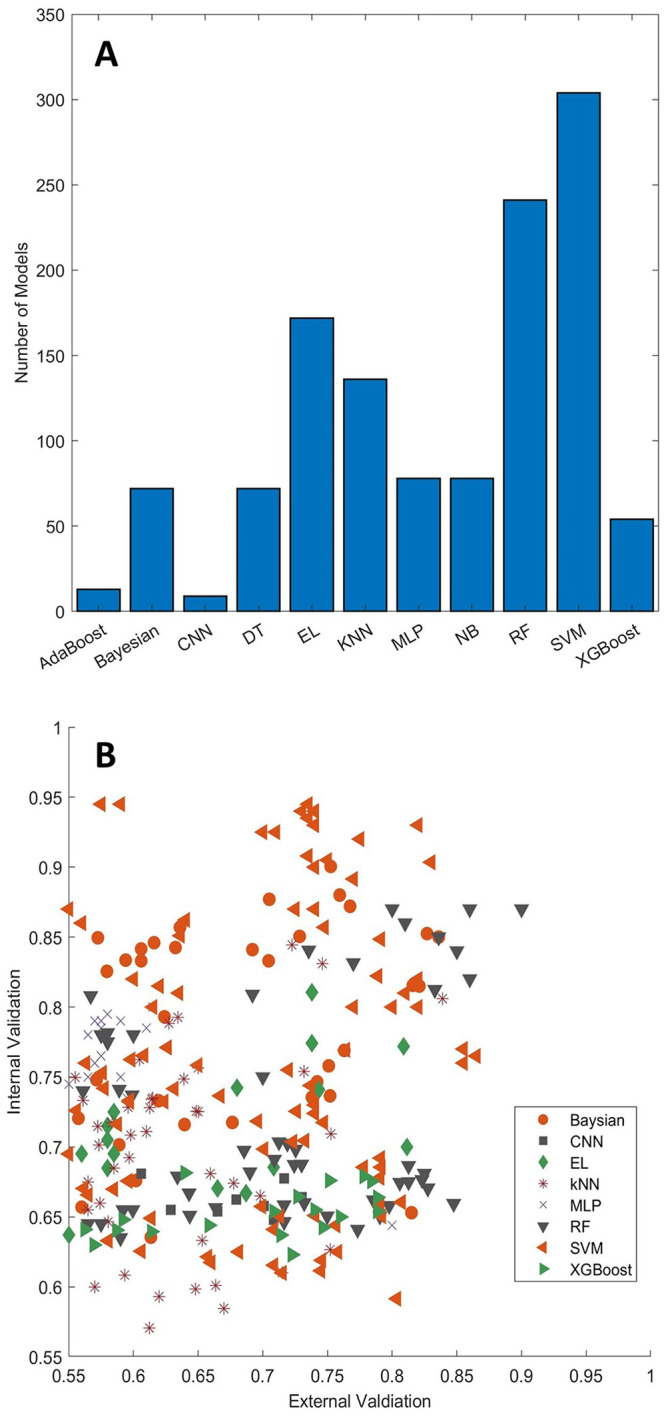
Figure 2. — Distribution of toxicity prediction models for machine learning and deep learning algorithms marked at the x-axis (a). Comparison between external validations (x-axis) and internal validations (y-axis) for toxicity prediction models (b). The machine learning and deep learning algorithms are depicted with different shapes and colors as shown in the figure legend. AdaBoost: adaptive boosting; CNN: convolutional neural network; DT: decision tree; EL: ensemble learning; KNN: k-nearest neighbors; MLP: multilayer perceptron; NB: Naïve Bayes; RF: random forest; SVM: support vector machine; XGBoost: extreme gradient boosting.

SVM is one of the most popular supervised ML algorithms and was introduced by Vapnik et al.¹¹⁵ based on the structural risk minimization principle. In SVM, chemicals described by the original input descriptors are mapped into a higher dimensional space using a kernel function, and a hyperplane is then identified in the mapped space to separate classes of chemicals. When training an SVM model, the algorithmic parameters such as the ones associated with kernel function are tuned to determine the optimal hyperplane that maximizes the distance between the hyperplane and the margin (samples are most close to the hyperplane, they form the support vector) of each class of chemicals. Since SVM can handle correlated descriptors and has good generalization performance, it has been widely used in the development of models for predicting toxicity of chemicals, with 304 models reported.^{18,25–27,29,32,34,35,64–70,82,89,93,101,116,117}

Decision tree (DT) is an upside-down tree-like classification and regression algorithm with the root on the top, leaf nodes at the bottom, and several layers of internal nodes in the middle. A path from the root to a leaf forms a branch which represents a series of decision rules used to classify chemicals. Since the decision rules can be easily retrieved from a DT model, chemical toxicity prediction models constructed with a DT algorithm are easy to interpret the predicted toxicity and intuitive to understand the importance of chemical features of the toxicity. However, the paths of decisions in a DT model use cutoffs for chemical features but do not take into consideration the values of chemical features. This results in chemicals that meet the same cutoffs but have very different feature values being assigned to the same class, which may make the performance of a DT model on testing not as good as in training. Therefore, relatively few prediction models are developed using DT in predictive toxicology, with only 72 models reported for predicting carcinogenicity,⁶⁷ genotoxicity,^74,92–94 hepatotoxicity,^25,33 and reprotoxicity.^18,90

An RF model is built based on DT models. It makes predictions by taking majority votes from its member DT models. In RF, chemicals and structural features are randomly selected from the training dataset to construct a set of DT models for making a prediction model. The consensus of DT models generated using different chemicals and structural features selected by randomization is expected to minimize the effect of overfitting of individual DT models and to improve prediction performance. For example, Fujita et al.⁹² developed both DT and RF models to evaluate the carcinogenicity of 230 chemicals. The balanced accuracy from the evaluation for the RF model was 0.755, which was substantially higher than the balanced accuracy of 0.54 for the DT model. Although RF is less interpretable, it is computationally efficient and has been very successful in developing classification models for a wide range of toxicity types.^{18,25,29,30,45,48,50,65,75,93,101,118}

Ensemble learning models that combine individual models other than DT models in RF have also been reported for predicting various toxicity endpoints. These ensemble learning models used majority voting of their individual models as the final predictions. Most of the ensemble learning models outperformed the individual models, especially when the individual models are diverse. The ensemble learning models given in Table 1 used combinations of individual models constructed from SVM, DT, kNN, and Naïve Bayes. Table 1 and Figure 2 showed that ensemble learning has been widely used in the predictive toxicology field, with 172 models published.^{28,29,33,48,50,51,65,74,116,119–121}

kNN is one of the simplest ML algorithms. In a kNN model, the activity of a chemical is predicted using k chemicals with the shortest distances to it among the training chemicals in the chemical space that is represented with a set of chemical descriptors. For classification, the class prediction for a chemical is usually determined by majority voting, that is, the class with most of its k-nearest chemicals. kNN algorithm is simple and easy to understand and prediction models constructed with kNN have high interpretability. Therefore, it has been widely used in predictive toxicology with 136 kNN models reported for predicting carconogenicty,^62,64,67 cardiotoxicity,^45,48,51 genotoxicity,⁹³ hepatotoxicity,^25,26,33 and reprotoxicity.^18,90

Artificial neural networks (ANNs) are a set of algorithms that are used to recognize underlying relationships in data through a process that mimics the function of biological NNs. There are three layers in an ANN: an input layer, a hidden layer, and an output layer. Each layer consists of neurons, and each neuron is connected to all the neurons in the next layer by weight. The weights are randomly chosen at the beginning of a training process and are then calculated to minimize errors between predicted values from the output layers and actual values. As an extension to ANNs, DNNs with multiple hidden layers have been successfully applied in many fields due to the increase in computational power. In a DNN, the earlier layers can learn low-level simple features, while the later layers can learn more complex features. This complex model architecture makes DL well suited to build complex relationships between chemical structures and toxic effects that traditional ML models are unable to handle. In the reported DL models for toxicity prediction, MLP and CNN are the most used algorithms, with 78 and 9 models reported, respectively. MLP is a popular DNN with feedforward NN that utilizes a supervised learning technique called backpropagation to recognize underlying relationships in data. MLP models have been developed for predicting cardiotoxity,^42,49 cytotoxicity,⁸³ genotoxicity,^78,93,119 hepatotoxicity,^26,29,33,34 oral toxicity,¹⁰¹ and reprotoxicity.¹⁸ CNN is a feedforward NN and typically consists of convolutional and pooling layers, which differs from MLP models. CNN has an advantage over traditional ANNs since it requires fewer free parameters. However, a large amount of data is required for training a CNN model. Therefore, compared with MLP models, fewer CNN models have been reported for toxicity assessment.^37,64 Recently, GCN has attracted a lot of attention for its application in the analysis of biomolecular structures, which can be represented as undirected graphs. In the graphical representation of a molecule, atoms are denoted as nodes and bonds as edges. Since GCN can directly process graph structures, it bypasses the limitation typically associated with conventional molecular descriptors. This inherent feature contributes to its enhanced performance in predictive tasks, especially in the toxicity prediction fields where various GCN-based models have been developed to address diverse endpoints. ^{42,77,122–124} For example, Kearnes et al. ¹²⁵ developed a GCN model to extract informative features from the graph-based representation of atoms and bonds. Furthermore, researchers have advanced GCN-based models, including graph attention CNN,¹²⁶ DeepAffnity,¹²⁴ MutagenPre-GCNN,⁷⁷ to improve predictive accuracy and identification of structurally significant features.

Figure 2(a) shows the numbers of models developed using different ML algorithms. SVM and RF are the most frequently used ML algorithms. Various validation methods such as holdout validation, cross validation, and external validation have been used for assessing the performance of those ML and DL models developed for predicting the toxicity of chemicals. In a holdout validation, the original dataset is split into a training set and a test dataset. A model is trained on the training dataset and evaluated on the test dataset. In a k-fold cross validation, the original dataset is first randomly divided into k groups. Then, k-1 groups are used to build a model, and the remaining group is used to evaluate the model. This process is iterated k times so that each of the k groups is used only once as the test set. In an external validation, an external dataset is used to validate the performance of the model developed with a training dataset.

As shown in Table 1, most studies used only internal validations (holdout and k-fold cross validation) to assess model performance. About 25% of the models were validated using both internal and external validations. Figure 2(b) compares the internal and external validation results. Not surprisingly, the internal validations had better performance than the external validations. Furthermore, the differences between internal and external validations are not dependent on the ML algorithms used for model development. The comparative analysis suggests that external validation should be used for validating the performance of ML and DL models developed for predicting the toxicity of chemicals. When an external dataset is not available, internal validation provides a useful estimation of model performance though internal validation usually overestimates model performance.

Datasets

ML and DL models are trained using known experimental data to learn the relationships between chemical structures and toxicity endpoints in the training chemicals. Therefore, the quality of experimental data used for training ML and DL models is important for the reliability of developed toxicity prediction models. Many toxicity studies collected experimental data from a variety of data sources and established databases to manage the collected data, including ToxCast/Tox21,¹²⁷ ChEMBL,⁴¹ ToxRefDB,¹²⁸ PubChem,⁴⁰ CPDB,⁵⁹ EDKB,¹²⁹ and EADB.⁵ Since these databases contain data that were generated from different experiments and in various formats, data processing and curation are needed to prepare datasets from these databases for developing ML and DL models. For example, datasets extracted from the ToxCast/Tox21 database have been used to develop models for predicting reprotoxicity,^128,130 hepatotoxicity,¹³¹ and other organ toxicity.^132,133 The datasets that have been used for developing toxicity prediction models are summarized below.

Compared with large datasets with billions or even trillions of data in image analysis, data size for the predictive toxicology field is typically small due to the high cost and time involved in performing toxicological experiments. Figure 3 shows the size distribution of the datasets that have been used in the development of ML and DL models for predicting various toxicity types. The largest dataset is the cytotoxicity dataset that has 62,655 compounds,⁸⁴ and few datasets contain more than 10,000 compounds. Most of the datasets have around 1000 chemicals. The sizes of most datasets are not large enough to develop accurate and reliable DL models. Therefore, most of the toxicity prediction models have been developed using ML algorithms (Figure 2[a]). There are more datasets for cardiotoxicity, carcinogenicity, and hepatotoxicity than other types of toxicity. The average data sizes for cardiotoxicity, hepatotoxicity, and carcinogenicity are 2053, 958, and 896, respectively.

Figure 3. — Histogram of sizes of the datasets used in the development of machine learning and deep learning models for toxicity prediction.

For cardiotoxicity, Cai et al,⁴² Chavan et al.,⁵¹ Karim et al.,¹²² and Doddareddy et al.,¹³⁴ built datasets by collecting data from BindingDB,³⁹ PubChem,⁴⁰ and ChEMBL⁴¹ databases, as well as from the literature. Some cardiotoxicity datasets have thousands of molecules with inhibitory activity of the hERG channel.^{45,46,48,54,134} It is interesting to note that DL models have been developed for some large cardiotoxicity datasets. For example, various DL algorithms were used in the development of hERG channel blockade prediction models based on 12,620 chemicals that were curated from multiple sources.¹²² Different chemical descriptors such as fingerprints and features vectorized from SMILES strings were used in those DL models. However, cross validations had an accuracy between 60% and 86%, and external validations resulted in an accuracy between 75% and 81% for the best models. Compared with ML models (Table 1), DL did not show advantages over ML for such size hERG inhibition datasets.

For hepatotoxicity, some datasets have been generated and curated in the last decade, including ones published by Chen et al.,²³ Liew et al.,¹²⁰ Fourches et al.,¹³⁵ Zhu et al.,¹³⁶ and Zhang et al.¹³⁷ These datasets served as important resources for developing hepatotoxicity prediction models. As hepatotoxicity is a major concern in drug safety evaluation, DILI in humans is the objective for most of the ML and DL models for predicting hepatotoxicity. DILI in humans is caused by diverse and complicated mechanisms. Thus, predicting DILI in humans is very challenging, and high-quality datasets are vital for developing reliable and accurate prediction models using ML and DL learning algorithms. The DILI datasets used in training the reported ML and DL prediction models were generated using various methods which can be categorized into three approaches. The first approach is based on DFA-approved drug labeling documents.^23,138 The second approach is based on drug safety reports such as the FDA adverse event reporting system¹³⁶ and Micromedex Healthcare Series reports on adverse reactions.¹²⁰ The third approach is to search publications in the literature such as MEDLINE abstracts¹³⁵ and publications.¹³⁷ Hepatotoxicity endpoints based on animal experiments were also curated for developing ML prediction models.¹³¹ A chemical could be annotated as hepatotoxic in one dataset, but as non-hepatotoxic in another dataset due to the difference in the approaches to define hepatotoxicity, not only leading to quality and reliability concerns on ML models based on such datasets but also resulting in the discordance in predictions from those models. Figure 4 shows comparisons between drugs in the datasets obtained from three sources: postmarket surveillance reports (282 drugs),¹³⁶ literature (937 drugs),¹³⁵ and drug labeling documents (387 drugs).¹³⁸ Of those drugs, 79 drugs are included in all three datasets, 184 drugs are common to the datasets obtained from postmarket surveillance reports and from literature, 100 drugs are included in the datasets obtained from postmarket surveillance reports and from drug labeling documents, and 206 drugs are shared by the datasets obtained from drug labeling documents and from literature. Comparing DILI annotations between datasets for the same drugs revealed that a considerable number of drugs have conflict DILI annotations, raising concerns on utilization of ML and DL models developed based on different datasets. Figure 5 compares DILI annotations of drugs common in pairs of datasets obtained from different sources. Close examination of the figure found that few drugs have conflict DILI annotations between drug labeling documents and postmarket surveillance reports, while a notably large number of drugs have conflict DILI annotations between literature and drug labeling documents and between literature and postmarket surveillance reports. The high conflict rates may be due to the many DILI annotations obtained from literature mining are based on animal experimental data, which are different from observations in humans in postmarket surveillance reports and drug labeling documents. Therefore, a high-quality benchmarking is urgently needed to enhance the development of ML and DL models for predicting hepatotoxicity in drug safety evaluation and chemical risk assessment.

Figure 4. — Venn diagram for comparison of DILI datasets generated from different sources. The dataset PMR obtained from postmarket surveillance reports is represented in the red circle; the dataset DLD generated from drug labeling documents is shown in the purple circle; and the dataset LIT, yielded through mining publications in the literature, is indicated in the green circle.

Figure 5. — Comparison of DILI annotations for the same drugs common to two datasets. Drugs in different categories of annotations are given in bars depicted by the y-axis. Drugs with the same DILI annotations are shown in blue bars. Drugs with conflict DILI annotations are plotted in the orange and green bars. DILI annotations for the same drugs are marked at the x-axis.

For carcinogenicity, most of the developed ML and DL models are based on the dataset extracted from the CPDB.⁵⁹ CPDB is a comprehensive resource of long-term animal carcinogenesis studies and collected results on various animal studies. Chemicals are labeled as carcinogens or non-carcinogens according to their carcinogenic potency (TD₅₀) values obtained in the studies. A chemical could be carcinogenic in one animal study but could be shown as non-carcinogenic in another animal study, raising challenges in classifying chemicals as carcinogens or non-carcinogens. Therefore, integrating results from different animal studies such as the dataset from combining rat, dog, and hamster studies⁶⁰ has not been well investigated in the development of ML and DL models for predicting the carcinogenic activity of chemicals. Most of the developed carcinogenesis prediction models were developed based on datasets of in vivo studies on rat from the CPDB. However, different datasets of rat carcinogenic activity were derived from the same CPDB data source without clear descriptions on how they are generated, and they were used in the development of ML and DL prediction models, resulting in different prediction performances. Our observations indicate that a well-annotated carcinogenic activity dataset is extremely important for developing reproducible and accurate prediction models using ML and DL algorithms. Furthermore, a clear description of the process that is used for generating a dataset is highly recommended in the publication of an ML or DL model for better understanding and applying the developed model in safety evaluation and risk assessment.

In addition to cardiotoxicity, hepatotoxicity, and carcinogenicity datasets, genotoxicity datasets are also characterized by their large size. Most mutagenicity datasets have been derived from the Hansen Ames Salmonella mutagenicity benchmark dataset with around 6500 compounds.⁷⁹ It is encouraging to find that, as shown in Figure 6, some ML and DL models developed for Ames mutagenicity prediction have balanced accuracy within the range of 0.80–0.85, which is the technical repeatability range of the Ames test.¹³⁹ Balanced accuracy is the mean of sensitivity and specificity and should be smaller than overall accuracy or concordance or technical repeatability. Thus, more ML and DL models performed similarly to laboratory tests, indicating well-developed and validated ML and DL models may be an attractive alternative method to the Ames test in genotoxicity assessment.

Figure 6. — Validation results of machine learning and deep learning models for predicting Ames mutagenicity. Balanced accuracy values from cross validations, holdout validations, and external validations are plotted as circles, diamonds, and triangles, respectively. The technical repeatability range for Ames test experiments is given by the two red dashed lines.

We examined the impact of data size on the performance of ML and DL models for toxicity prediction. If balanced accuracy or sensitivity and specificity were not provided, models were excluded from the comparison in Table 1. As shown in Table 1, models developed using larger datasets did not outperform the models developed using smaller datasets. Several factors may contribute to this observation. First, the quality of large datasets is a critical factor influencing model performance. Second, large datasets often encompass a more diverse space of chemicals, making it inherently challenging to develop models that exhibit consistent and robust performance across such diverse data. For hepatotoxicity, the balanced accuracy is around 0.7 for models developed with datasets of different sizes. Compared with ML and DL models for predicting other toxicity types, prediction accuracy values of the models for predicting hepatotoxicity and carcinogenicity are low and have a large variation, while cardiotoxicity and reprotoxicity models have good performance, and balanced accuracy of some models reached above 0.9. The low model performance for carcinogenicity and hepatotoxicity may be due to diverse and complex mechanisms for such toxicity obtained from animal experiments and observed in humans, and thus the quality of the datasets is difficult to ensure.

Concluding remarks and future perspective

Recently, many ML models have been developed for predicting various chemical toxicity endpoints. The model performance could be impacted by various factors such as hyperparameters, descriptors, algorithms, and validation methods. It is challenging to incorporate all these factors for comparison. Therefore, this review focused on three key factors: toxicity types, algorithms, and validation methods. Using this approach, we sought to compare model performance within a manageable framework. This review investigated the impact of these factors on model performance. Although the direct comparability of performance may be challenging, our review highlighted the impact of these factors on the model performance.

Regarding toxicity types, this review focuses on some extensively explored toxicity types including carcinogenicity, cytotoxicity, genotoxicity, hepatotoxicity, oral toxicity, and reprotoxicity. Many ML and DL models have been developed for predicting hepatotoxicity, carcinogenicity, and cardiotoxicity due to the importance of these toxicity types. Most ML and DL models for cardiotoxicity prediction are based on in vitro hERG inhibitory data and have very good predictive performance, while the majority of the ML and DL models for predicting hepatotoxicity and carcinogenicity have poor performance as they are trained with in vivo animal testing data or text mining results from documents such as adverse reactions in case reports and regulatory documents as well as publications in the literature. Compared with in vitro experiments, in vivo animal testing is much more expensive. Therefore, it is a huge challenge to obtain large datasets of in vivo toxicity data for developing accurate and reliable prediction models using ML and DL algorithms.

Another challenge for predictive toxicology is the lack of high-quality data for developing ML and DL models since the reliability of ML and DL models depends on the quality of toxicity data and the diversity of chemicals for training the models. Despite the collaborative efforts within the research community,^88,140 establishing benchmark datasets for all types of toxicity endpoints is an important task for future application of ML and DL in predictive toxicology. Due to differences in in vitro assays and in vivo experiments, one of the most important quality issues is to integrate toxicity data from different experiments for the same toxicity types and endpoints which are often not consistent. Another data quality issue is high error rate of data curated from data mining, which will be extremely vital in the future as data volume will become larger and larger.

In predictive toxicology, the selection of molecular representation is one of the most important steps. Molecular representation can take various forms, including labeled molecular graphs where atoms are represented as nodes and bonds as edges, or molecular fingerprints, which indicate the presence or absence of specific substructures. As shown in Table 1, commonly used descriptors include constitutional, topological, geometrical, quantum chemical, and molecular properties as well as fingerprints such as MACCS Keys, PubChem Substructures Fingerprints (PCFP), and Extended Connectivity Fingerprints (ECFP). These descriptors are typically calculated using well-established software tools such as MOE,¹⁴¹ PaDEL,¹⁴² Dragon,¹⁴³ and Mold2.¹⁴⁴ The combination of molecular descriptors and fingerprints is a common practice for molecular representation. An equally critical step is the selection of the most relevant descriptors from a large feature set. Given that irrelevant descriptors could adversely affect prediction accuracy, various feature selection steps, including stepwise selection, pairwise decorrelation, low variance removal, and high correlation coefficient removal, have been employed to effectively eliminate redundant descriptors and improve prediction accuracy. It is worth noting that the necessity of conventional feature selection techniques is reduced for DL methods, which are capable of high-dimensional data reduction.^37,43,77,104 For example, in the case of GCN, the molecular graph can be used as direct input and there is no need for manual curation of descriptors. ^77,124,126

In predictive toxicology, supervised learning still plays a crucial role by primarily focusing on the classification of input data into distinct toxicity categories or the prediction of quantitative toxicity values. In supervised learning, models are trained using labeled datasets that include well-defined input parameters like molecular descriptors, paired with corresponding output labels or toxicity values. Model performance is evaluated by comparing predictions with experimental labels. In a different way, unsupervised learning models are trained using unlabeled data, with the primary goal of uncovering hidden patterns and clusters within the dataset. Self-supervised learning, a subset of unsupervised learning, could improve model performance by utilizing unlabeled data to generate labels for model training. In contrast, semi-supervised learning utilizes both labeled and unlabeled data to enhance model performance. It is worth noting that unsupervised and semi-supervised models are still relatively less prevalent when compared with supervised models. However, unsupervised learning, semi-supervised learning, and self-supervised learning offer great advantages for handling vast amounts of unlabeled data to improve toxicity prediction accuracy. Unsupervised learning has the potential to reveal concealed toxicity patterns and associations that may be ignored by supervised approaches. This is particularly useful in toxicity assessments when labeled data are limited. Moreover, given the dynamic nature of toxicity datasets characterized by the emergence of novel substances, unsupervised and semi-supervised models demonstrate the adaptability to accommodate evolving datasets and maintain the ongoing accuracy of toxicity predictions.

Despite these challenges in the applications of ML and DL for toxicity prediction, great progress has been made in building toxicity prediction models using various ML and DL algorithms. Among the algorithms used in the developed models, SVM and RF are the most used algorithms and the models built with SVM and RF generally performed well. In the future, SVM and RF may continue to be popular ML algorithms in predictive toxicology, but more toxicity prediction models are expected to be developed using other ML algorithms. Compared with ML, DL is less used in the development of models for predicting toxicity. For some cases, the use of DL improved model prediction accuracy, but, for most cases, the performance of DL models did not show a substantial improvement. This may be due to the lack of large datasets on which DL heavily relies. However, DL has great potential, and we expect more DL models will be developed to improve toxicity prediction in the future when more time and effort are invested in collecting high-quality data.

Model interpretability is important for the utilization of ML and DL models. The ability to understand the rationale behind specific model predictions is essential, not only for regulatory compliance but also for gaining insight into the toxicological mechanisms. However, achieving interpretability in DL and ML can be challenging, given that models are often regarded as black boxes with their decision-making process unclear or unexplained. Conventional tree-based models, such as DT or RF, are inherently interpretable due to their transparent decision paths. One can trace and understand the decision-making process by following the rules encoded within the structure of a tree-based model. However, DNN poses a great challenge to interpretability due to its complex architecture characterized by numerous layers and millions of parameters. The complexity makes it challenging to identify the specific features or interactions responsible for a particular prediction. Nevertheless, there has been remarkable progress in developing various methods and techniques to enhance model transparency and interpretability. For example, feature importance analysis, rule extraction methods, and the design of interpretable architectures have been developed to help models become more transparent and interpretable while handling complex problems effectively.

Acknowledgments

This research was supported in part by an appointment to the Research Participation Program at the National Center for Toxicological Research (Meng Song, Zoe Li, and Md Kamrul Hasan Khan), administered by the Oak Ridge Institute for Science and Education through an interagency agreement between the U.S. Department of Energy and the U.S. Food and Drug Administration.

Footnotes

Authors’ contributions: WG, JL, FD, MS, ZL, MK, and HH reviewed the literature. WG and HH wrote the first draft. TP revised the manuscript. All authors have reviewed and agreed to the published version of the manuscript.

The author(s) declared no potential conflicts of interest with respect to the research, authorship, and/or publication of this article.

Funding: The author(s) received no financial support for the research, authorship, and/or publication of this article.

Disclaimer: This article reflects the views of the authors and does not necessarily reflect those of the U.S. Food and Drug Administration.

ORCID iDs: Wenjing Guo Inline graphic https://orcid.org/0000-0002-0814-6982

Jie Liu Inline graphic https://orcid.org/0000-0001-6988-5773

Md Kamrul Hasan Khan Inline graphic https://orcid.org/0009-0004-9835-5594

Huixiao Hong Inline graphic https://orcid.org/0000-0001-8087-3968

References

1. Hong H, Thakkar S, Chen M, Tong W. Development of decision forest models for prediction of drug-induced liver injury in humans using a large set of FDA-approved drugs. Sci Rep 2017;7:17311. [DOI] [PMC free article] [PubMed] [Google Scholar]
2. Ng HW, Doughty SW, Luo H, Ye H, Ge W, Tong W, Hong H. Development and validation of decision forest model for estrogen receptor binding prediction of chemicals using large data sets. Chem Res Toxicol 2015;28:2343–51 [DOI] [PubMed] [Google Scholar]
3. Idakwo G, Luttrell J, Chen M, Hong H, Zhou Z, Gong P, Zhang C. A review on machine learning methods for in silico toxicity prediction. J Environ Sci Health C Environ Carcinog Ecotoxicol Rev 2018;36:169–91 [DOI] [PubMed] [Google Scholar]
4. Luo H, Ye H, Ng HW, Shi L, Tong W, Mendrick DL, Hong H. Machine learning methods for predicting HLA-peptide binding activity. Bioinform Biol Insights 2015;9:21–9 [DOI] [PMC free article] [PubMed] [Google Scholar]
5. Shen J, Xu L, Fang H, Richard AM, Bray JD, Judson RS, Zhou G, Colatsky TJ, Aungst JL, Teng C, Harris SC, Ge W, Dai SY, Su Z, Jacobs AC, Harrouk W, Perkins R, Tong W, Hong H. Eadb: an estrogenic activity database for assessing potential endocrine activity. Toxicol Sci 2013;135:277–91 [DOI] [PubMed] [Google Scholar]
6. Hong H, Tong W, Xie Q, Fang H, Perkins R. An in silico ensemble method for lead discovery: decision forest. SAR QSAR Environ Res 2005;16:339–47 [DOI] [PubMed] [Google Scholar]
7. Idakwo G, Luttrell J IV, Chen M, Hong H, Gong P, Zhang C. A review of feature reduction methods for qsar-based toxicity prediction. In: Hong H. (ed.) Advances in computational toxicology. Cham: Springer, 2019, pp.119–39 [Google Scholar]
8. Hong H, Zhu J, Chen M, Gong P, Zhang C, Tong W. Quantitative structure–activity relationship models for predicting risk of drug-induced liver injury in humans. In: Chen M, Will Y. (eds) Drug-induced liver toxicity. New York: Humana, 2018, pp.77–100 [Google Scholar]
9. Sakkiah S, Selvaraj C, Gong P, Zhang C, Tong W, Hong H. Development of estrogen receptor beta binding prediction model using large sets of chemicals. Oncotarget 2017;8:92989–3000 [DOI] [PMC free article] [PubMed] [Google Scholar]
10. Wang Z, Chen J, Hong H. Developing QSAR models with defined applicability domains on pparγ binding affinity using large data sets and machine learning algorithms. Environ Sci Technol 2021;55:6857–66 [DOI] [PubMed] [Google Scholar]
11. Idakwo G, Thangapandian S, Luttrell J, Li Y, Wang N, Zhou Z, Hong H, Yang B, Zhang C, Gong P. Structure–activity relationship-based chemical classification of highly imbalanced Tox21 datasets. J Cheminform 2020;12:1–19 [DOI] [PMC free article] [PubMed] [Google Scholar]
12. Maxwell A, Li R, Yang B, Weng H, Ou A, Hong H, Zhou Z, Gong P, Zhang C. Deep learning architectures for multi-label classification of intelligent health risk prediction. BMC Bioinform 2017;18:121–31 [DOI] [PMC free article] [PubMed] [Google Scholar]
13. Tang W, Chen J, Wang Z, Xie H, Hong H. Deep learning for predicting toxicity of chemicals: a mini review. J Environ Sci Health C Environ Carcinog Ecotoxicol Rev 2018;36:252–71 [DOI] [PubMed] [Google Scholar]
14. Raies AB, Bajic VB. In silico toxicology: computational methods for the prediction of chemical toxicity. Wiley Interdiscip Rev Comput Mol Sci 2016;6:147–72 [DOI] [PMC free article] [PubMed] [Google Scholar]
15. Huang Y, Li X, Xu S, Zheng H, Zhang L, Chen J, Hong H, Kusko R, Li R. Quantitative structure–activity relationship models for predicting inflammatory potential of metal oxide nanoparticles. Environ Health Perspect 2020;128:067010. [DOI] [PMC free article] [PubMed] [Google Scholar]
16. Ng HW, Shu M, Luo H, Ye H, Ge W, Perkins R, Tong W, Hong H. Estrogenic activity data extraction and in silico prediction show the endocrine disruption potential of bisphenol a replacement compounds. Chem Res Toxicol 2015;28:1784–95 [DOI] [PubMed] [Google Scholar]
17. Feng H, Zhang L, Li S, Liu L, Yang T, Yang P, Zhao J, Arkin IT, Liu H. Predicting the reproductive toxicity of chemicals using ensemble learning methods and molecular fingerprints. Toxicol Lett 2021;340:4–14 [DOI] [PubMed] [Google Scholar]
18. Jiang C, Yang H, Di P, Li W, Tang Y, Liu G. In silico prediction of chemical reproductive toxicity using machine learning. J Appl Toxicol 2019;39:844–54 [DOI] [PubMed] [Google Scholar]
19. Segall MD, Barber C. Addressing toxicity risk when designing and selecting compounds in early drug discovery. Drug Discov Today 2014;19:688–93 [DOI] [PubMed] [Google Scholar]
20. Andrade RJ, Chalasani N, Björnsson ES, Suzuki A, Kullak-Ublick GA, Watkins PB, Devarbhavi H, Merz M, Lucena MI, Kaplowitz N, Aithal GP. Drug-induced liver injury. Nature Reviews Disease Primers 2019;5:58. [DOI] [PubMed] [Google Scholar]
21. Kullak-Ublick GA, Andrade RJ, Merz M, End P, Benesic A, Gerbes AL, Aithal GP. Drug-induced liver injury: recent advances in diagnosis and risk assessment. Gut 2017;66:1154–64 [DOI] [PMC free article] [PubMed] [Google Scholar]
22. Kuna L, Bozic I, Kizivat T, Bojanic K, Mrso M, Kralj E, Smolic R, Wu GY, Smolic M. Models of Drug Induced Liver Injury (DILI)—current issues and future perspectives. Curr Drug Metab 2018;19:830–8 [DOI] [PMC free article] [PubMed] [Google Scholar]
23. Chen M, Suzuki A, Thakkar S, Yu K, Hu C, Tong W. DILIrank: the largest reference drug list ranked by the risk for developing drug-induced liver injury in humans. Drug Discov Today 2016;21:648–53 [DOI] [PubMed] [Google Scholar]
24. Minerali E, Foil DH, Zorn KM, Lane TR, Ekins S. Comparing machine learning algorithms for predicting Drug-Induced Liver Injury (DILI). Mol Pharm 2020;17:2628–37 [DOI] [PMC free article] [PubMed] [Google Scholar]
25. Li X, Chen Y, Song X, Zhang Y, Li H, Zhao Y. The development and application of in silico models for drug induced liver injury. RSC Adv 2018;8:8101–11 [DOI] [PMC free article] [PubMed] [Google Scholar]
26. Li T, Tong W, Roberts R, Liu Z, Thakkar S. Deep learning on high-throughput transcriptomics to predict drug-induced liver injury. Front Bioeng Biotechnol 2020;8:562677. [DOI] [PMC free article] [PubMed] [Google Scholar]
27. Su R, Wu H, Xu B, Liu X, Wei L. Developing a multi-dose computational model for drug-induced hepatotoxicity prediction based on toxicogenomics data. IEEE/ACM Trans Comput Biol Bioinform 2019;16:1231–9 [DOI] [PubMed] [Google Scholar]
28. Alves VM, Golbraikh A, Capuzzi SJ, Liu K, Lam WI, Korn DR, Pozefsky D, Andrade CH, Muratov EN, Tropsha A. Multi-Descriptor Read across (MuDRA): a simple and transparent approach for developing accurate quantitative structure–activity relationship models. J Chem Inf Model 2018;58:1214–23 [DOI] [PMC free article] [PubMed] [Google Scholar]
29. Adeluwa T, McGregor BA, Guo K, Hur J. Predicting drug-induced liver injury using machine learning on a diverse set of predictors. Front Pharmacol 2021;12:648805. [DOI] [PMC free article] [PubMed] [Google Scholar]
30. Banerjee P, Eckert AO, Schrey AK, Preissner R. Protox-Ii: a webserver for the prediction of toxicity of chemicals. Nucleic Acids Res 2018;46:W257–163 [DOI] [PMC free article] [PubMed] [Google Scholar]
31. Zhu XW, Xin YJ, Chen QH. Chemical and in vitro biological information to predict mouse liver toxicity using recursive random forests. SAR QSAR Environ Res 2016;27:559–72 [DOI] [PubMed] [Google Scholar]
32. Liu A, Walter M, Wright P, Bartosik A, Dolciami D, Elbasir A, Yang H, Bender A. Prediction and mechanistic analysis of Drug-Induced Liver Injury (DILI) based on chemical structure. Biol Direct 2021;16:6. [DOI] [PMC free article] [PubMed] [Google Scholar]
33. He S, Ye T, Wang R, Zhang C, Zhang X, Sun G, Sun X. An in silico model for predicting drug-induced hepatotoxicity. Int J Mol Sci 2019;20:1897. [DOI] [PMC free article] [PubMed] [Google Scholar]
34. Feng C, Chen H, Yuan X, Sun M, Chu K, Liu H, Rui M. Gene expression data based deep learning model for accurate prediction of drug-induced liver injury in advance. J Chem Inf Model 2019;59:3240–50 [DOI] [PubMed] [Google Scholar]
35. Hammann F, Schöning V, Drewe J. Prediction of clinically relevant drug-induced liver injury from structure using machine learning. J Appl Toxicol 2019;39:412–9 [DOI] [PubMed] [Google Scholar]
36. Xu Y, Dai Z, Chen F, Gao S, Pei J, Lai L. Deep learning for drug-induced liver injury. J Chem Inf Model 2015;55:2085–93 [DOI] [PubMed] [Google Scholar]
37. Nguyen-Vo TH, Nguyen L, Do N, Le PH, Nguyen TN, Nguyen BP, Le L. Predicting drug-induced liver injury using convolutional neural network and molecular fingerprint-embedded features. ACS Omega 2020;5:25432–9 [DOI] [PMC free article] [PubMed] [Google Scholar]
38. Recanatini M, Poluzzi E, Masetti M, Cavalli A, De Ponti F. Qt Prolongation through hERG K(+) channel blockade: current knowledge and strategies for the early prediction during drug development. Med Res Rev 2005;25:133–66 [DOI] [PubMed] [Google Scholar]
39. Gilson MK, Liu T, Baitaluk M, Nicola G, Hwang L, Chong J. Bindingdb in 2015: a public database for medicinal chemistry, computational chemistry and systems pharmacology. Nucleic Acids Res 2016;44:D1045–D1153 [DOI] [PMC free article] [PubMed] [Google Scholar]
40. Wang Y, Xiao J, Suzek TO, Zhang J, Wang J, Zhou Z, Han L, Karapetyan K, Dracheva S, Shoemaker BA, Bolton E, Gindulyte A, Bryant SH. Pubchem’s bioassay database. Nucleic Acids Res 2011;40:D400–D412 [DOI] [PMC free article] [PubMed] [Google Scholar]
41. Gaulton A, Bellis LJ, Bento AP, Chambers J, Davies M, Hersey A, Light Y, McGlinchey S, Michalovich D, Al-Lazikani B, Overington JP. Chembl: a large-scale bioactivity database for drug discovery. Nucleic Acids Res 2012;40:D1100–17 [DOI] [PMC free article] [PubMed] [Google Scholar]
42. Cai C, Guo P, Zhou Y, Zhou J, Wang Q, Zhang F, Fang J, Cheng F. Deep learning-based prediction of drug-induced cardiotoxicity. J Chem Inf Model 2019;59:1073–84 [DOI] [PMC free article] [PubMed] [Google Scholar]
43. Ryu JY, Lee MY, Lee JH, Lee BH, Oh KS. Deephit: a deep learning framework for prediction of hERG-induced cardiotoxicity. Bioinformatics 2020;36:3049–55 [DOI] [PubMed] [Google Scholar]
44. Wang S, Li Y, Wang J, Chen L, Zhang L, Yu H, Hou T. Admet evaluation in drug discovery. 12. Development of binary classification models for prediction of hERG potassium channel blockage. Mol Pharm 2012;9:996–1010 [DOI] [PMC free article] [PubMed] [Google Scholar]
45. Siramshetty VB, Chen Q, Devarakonda P, Preissner R. The catch-22 of predicting hERG blockade using publicly accessible bioactivity data. J Chem Inf Model 2018;58:1224–33 [DOI] [PubMed] [Google Scholar]
46. Shen M-y, Su B-H, Esposito EX, Hopfinger AJ, Tseng YJ. A comprehensive support vector machine binary hERG classification model based on extensive but biased end point hERG data sets. Chem Res Toxicol 2011;24:934–49 [DOI] [PubMed] [Google Scholar]
47. Lee HM, Yu MS, Kazmi SR, Oh SY, Rhee KH, Bae MA, Lee BH, Shin DS, Oh KS, Ceong H, Lee D, Na D. Computational determination of hERG-related cardiotoxicity of drug candidates. BMC Bioinform 2019;20:250. [DOI] [PMC free article] [PubMed] [Google Scholar]
48. Li X, Zhang Y, Li H, Zhao Y. Modeling of the hERG K+ channel blockage using online chemical database and modeling environment (OCHEM). Mol Inform 2017;36:12. [DOI] [PubMed] [Google Scholar]
49. Zhang Y, Zhao J, Wang Y, Fan Y, Zhu L, Yang Y, Chen X, Lu T, Chen Y, Liu H. Prediction of hERG K+ channel blockage using deep neural networks. Chem Biol Drug Des 2019;94:1973–85 [DOI] [PubMed] [Google Scholar]
50. Liu M, Zhang L, Li S, Yang T, Liu L, Zhao J, Liu H. Prediction of hERG potassium channel blockage using ensemble learning methods and molecular fingerprints. Toxicol Lett 2020;332:88–96 [DOI] [PubMed] [Google Scholar]
51. Chavan S, Abdelaziz A, Wiklander JG, Nicholls IA. A K-nearest neighbor classification of hERG K+ channel blockers. J Comput Aided Mol Des 2016;30:229–36 [DOI] [PMC free article] [PubMed] [Google Scholar]
52. Chen Y, Yu X, Li W, Tang Y, Liu G. In silico prediction of hERG blockers using machine learning and deep learning approaches. J Appl Toxicol 2023;43:1462–75 [DOI] [PubMed] [Google Scholar]
53. Kim H, Park M, Lee I, Nam H. Bayesherg: a robust, reliable and interpretable deep learning model for predicting hERG channel blockers. Brief Bioinform 2022;23:bbac211 [DOI] [PubMed] [Google Scholar]
54. Zhang C, Zhou Y, Gu S, Wu Z, Wu W, Liu C, Wang K, Liu G, Li W, Lee PW, Tang Y. In silico prediction of hERG potassium channel blockage by chemical category approaches. Toxicol Res 2016;5:570–82 [DOI] [PMC free article] [PubMed] [Google Scholar]
55. Liu LL, Lu J, Lu Y, Zheng MY, Luo XM, Zhu WL, Jiang HL, Chen KX. Novel Bayesian classification models for predicting compounds blocking hERG potassium channels. Acta Pharmacol Sin 2014;35:1093–102 [DOI] [PMC free article] [PubMed] [Google Scholar]
56. Ye L, Ngan DK, Xu T, Liu Z, Zhao J, Sakamuru S, Zhang L, Zhao T, Xia M, Simeonov A, Huang R. Prediction of drug-induced liver injury and cardiotoxicity using chemical structure and in vitro assay data. Toxicol Appl Pharmacol 2022;454:116250. [DOI] [PMC free article] [PubMed] [Google Scholar]
57. Mamoshina P, Bueno-Orovio A, Rodriguez B. Dual transcriptomic and molecular machine learning predicts all major clinical forms of drug cardiotoxicity. Front Pharmacol 2020;11:639. [DOI] [PMC free article] [PubMed] [Google Scholar]
58. Jacobs AC, Brown PC. Regulatory forum opinion piece*: transgenic/alternative carcinogenicity assays: a retrospective review of studies submitted to CDER/FDA 1997-2014. Toxicol Pathol 2015;43:605–10 [DOI] [PubMed] [Google Scholar]
59. Fitzpatrick RB. CPDB: carcinogenic potency database. Med Ref Serv Q 2008;27:303–11 [DOI] [PubMed] [Google Scholar]
60. Moorthy NSHN, Kumar S, Poongavanam V. Classification of carcinogenic and mutagenic properties using machine learning method. Comput Toxicol 2017;3:33–43 [Google Scholar]
61. Guan D, Fan K, Spence I, Matthews S. Combining machine learning models of in vitro and in vivo bioassays improves rat carcinogenicity prediction. Regul Toxicol Pharmacol 2018;94:8–15 [DOI] [PubMed] [Google Scholar]
62. Zhu H, Rusyn I, Richard A, Tropsha A. Use of cell viability assay data improves the prediction accuracy of conventional quantitative structure–activity relationship models of animal carcinogenicity. Environ Health Perspect 2008;116:506–13 [DOI] [PMC free article] [PubMed] [Google Scholar]
63. Zhang H, Cao ZX, Li M, Li YZ, Peng C. Novel naïve bayes classification models for predicting the carcinogenicity of chemicals. Food Chem Toxicol 2016;97:141–9 [DOI] [PubMed] [Google Scholar]
64. Wang YW, Huang L, Jiang SW, Li K, Zou J, Yang SY. Capscarcino: a novel sparse data deep learning tool for predicting carcinogens. Food Chem Toxicol 2020;135:110921. [DOI] [PubMed] [Google Scholar]
65. Zhang L, Ai H, Chen W, Yin Z, Hu H, Zhu J, Zhao J, Zhao Q, Liu H, CarcinoPred-EL: novel models for predicting the carcinogenicity of chemicals using molecular fingerprints and ensemble learning methods. Sci Rep 2017;7:2118. [DOI] [PMC free article] [PubMed] [Google Scholar]
66. Zhong M, Nie X, Yan A, Yuan Q. Carcinogenicity prediction of noncongeneric chemicals by a support vector machine. Chem Res Toxicol 2013;26:741–9 [DOI] [PubMed] [Google Scholar]
67. Li X, Du Z, Wang J, Wu Z, Li W, Liu G, Shen X, Tang Y. In silico estimation of chemical carcinogenicity with binary and ternary classification methods. Mol Inform 2015;34:228–35 [DOI] [PubMed] [Google Scholar]
68. Luan F, Zhang R, Zhao C, Yao X, Liu M, Hu Z, Fan B. Classification of the carcinogenicity of N-nitroso compounds based on support vector machines and linear discriminant analysis. Chem Res Toxicol 2005;18:198–203 [DOI] [PubMed] [Google Scholar]
69. Cao DS, Zhao JC, Yang YN, Zhao CX, Yan J, Liu S, Hu QN, Xu QS, Liang YZ. In silico toxicity prediction by support vector machine and smiles representation-based string kernel. SAR QSAR Environ Res 2012;23:141–53 [DOI] [PubMed] [Google Scholar]
70. Tan NX, Rao HB, Li ZR, Li XY. Prediction of chemical carcinogenicity by machine learning approaches. SAR QSAR Environ Res 2009;20:27–75 [DOI] [PubMed] [Google Scholar]
71. Ames BN, McCann J, Yamasaki E. Methods for detecting carcinogens and mutagens with the salmonella/mammalian-microsome mutagenicity Test. Mutat Res 1975;31:347–64 [DOI] [PubMed] [Google Scholar]
72. Chakravarti SK, Alla SRM. Descriptor free QSAR modeling using deep learning with long short-term memory neural networks. Front Artif Intell 2019;2:17. [DOI] [PMC free article] [PubMed] [Google Scholar]
73. Xu C, Cheng F, Chen L, Du Z, Li W, Liu G, Lee PW, Tang Y. In silico prediction of chemical ames mutagenicity. J Chem Inf Model 2012;52:2840–7 [DOI] [PubMed] [Google Scholar]
74. García G, García-Pedrajas N, Ruiz I, Gómez-Nieto M. An ensemble approach for in silico prediction of ames mutagenicity. J Math Chem 2018;56:2085–98 [Google Scholar]
75. Zhang J, Mucs D, Norinder U, Svensson F. Lightgbm: an effective and scalable algorithm for prediction of chemical toxicity–application to the Tox21 and mutagenicity data sets. J Chem Inf Model 2019;59:4150–8 [DOI] [PubMed] [Google Scholar]
76. Zhang H, Kang YL, Zhu YY, Zhao KX, Liang JY, Ding L, Zhang TG, Zhang J. Novel naïve bayes classification models for predicting the chemical ames mutagenicity. Toxicol in Vitro 2017;41:56–63 [DOI] [PubMed] [Google Scholar]
77. Li S, Zhang L, Feng H, Meng J, Xie D, Yi L, Arkin IT, Liu H. Mutagenpred-Gcnns: a graph convolutional neural network-based classification model for mutagenicity prediction with data-driven molecular fingerprints. Interdiscip Sci 2021;13:25–33 [DOI] [PubMed] [Google Scholar]
78. Sharma A, Kumar R, Varadwaj PK, Ahmad A, Ashraf GM. A comparative study of support vector machine, artificial neural network and bayesian classifier for mutagenicity prediction. Interdiscip Sci 2011;3:232–9 [DOI] [PubMed] [Google Scholar]
79. Hansen K, Mika S, Schroeter T, Sutter A, ter Laak A, Steger-Hartmann T, Heinrich N, Müller KR. Benchmark data set for in silico prediction of ames mutagenicity. J Chem Inf Model 2009;49:2077–81 [DOI] [PubMed] [Google Scholar]
80. Riss TL, Moravec RA, Niles AL. Cytotoxicity testing: measuring viable cells, dead cells, and detecting mechanism of cell death. Methods Mol Biol 2011;740:103–14 [DOI] [PubMed] [Google Scholar]
81. Svensson F, Norinder U, Bender A. Modelling compound cytotoxicity using conformal prediction and pubchem hts data. Toxicol Res 2017;6:73–80 [DOI] [PMC free article] [PubMed] [Google Scholar]
82. Chang C-Y, Hsu M-T, Esposito EX, Tseng YJ. Oversampling to overcome overfitting: exploring the relationship between data set composition, molecular descriptors, and predictive modeling methods. J Chem Inf Model 2013;53:958–71 [DOI] [PubMed] [Google Scholar]
83. Webel HE, Kimber TB, Radetzki S, Neuenschwander M, Nazaré M, Volkamer A. Revealing cytotoxic substructures in molecules using deep learning. J Comput Aided Mol Des 2020;34:731–46 [DOI] [PMC free article] [PubMed] [Google Scholar]
84. Yin Z, Ai H, Zhang L, Ren G, Wang Y, Zhao Q, Liu H. Predicting the cytotoxicity of chemicals using ensemble learning methods and molecular fingerprints. J Appl Toxicol 2019;39:1366–77 [DOI] [PubMed] [Google Scholar]
85. Mervin LH, Cao Q, Barrett IP, Firth MA, Murray D, McWilliams L, Haddrick M, Wigglesworth M, Engkvist O, Bender A. Understanding cytotoxicity and cytostaticity in a high-throughput screening collection. ACS Chem Biol 2016;11:3007–23 [DOI] [PubMed] [Google Scholar]
86. OECD. Test No. 414: Prenatal Developmental Toxicity Study. 2018
87. Piersma AH. Validation of alternative methods for developmental toxicity testing. Toxicol Lett 2004;149:147–53 [DOI] [PubMed] [Google Scholar]
88. Mansouri K, Abdelaziz A, Rybacka A, Roncaglioni A, Tropsha A, Varnek A, Zakharov A, Worth A, Richard AM, Grulke CM, Trisciuzzi D, Fourches D, Horvath D, Benfenati E, Muratov E, Wedebye EB, Grisoni F, Mangiatordi GF, Incisivo GM, Hong H, Ng HW, Tetko IV, Balabin I, Kancherla J, Shen J, Burton J, Nicklaus M, Cassotti M, Nikolov NG, Nicolotti O, Andersson PL, Zang Q, Politi R, Beger RD, Todeschini R, Huang R, Farag S, Rosenberg SA, Slavov S, Hu X, Judson RS. CERAPP: collaborative estrogen receptor activity prediction project. Environ Health Perspect 2016;124:1023–33 [DOI] [PMC free article] [PubMed] [Google Scholar]
89. Gunturi SB, Ramamurthi N. A novel approach to generate robust classification models to predict developmental toxicity from imbalanced datasets. SAR QSAR Environ Res 2014;25:711–27 [DOI] [PubMed] [Google Scholar]
90. Zhang H, Mao J, Qi HZ, Ding L. In silico prediction of drug-induced developmental toxicity by using machine learning approaches. Mol Divers 2020;24:1281–90 [DOI] [PubMed] [Google Scholar]
91. Zhang H, Ren JX, Kang YL, Bo P, Liang JY, Ding L, Kong WB, Zhang J. Development of novel in silico model for developmental toxicity assessment by using naïve bayes classifier method. Reprod Toxicol 2017;71:8–15 [DOI] [PubMed] [Google Scholar]
92. Fujita Y, Honda H, Yamane M, Morita T, Matsuda T, Morita O. A decision tree-based integrated testing strategy for tailor-made carcinogenicity evaluation of test substances using genotoxicity test results and chemical spaces. Mutagenesis 2019;34:101–9 [DOI] [PubMed] [Google Scholar]
93. Fan D, Yang H, Li F, Sun L, Di P, Li W, Tang Y, Liu G. In silico prediction of chemical genotoxicity using machine learning methods and structural alerts. Toxicol Res 2018;7:211–20 [DOI] [PMC free article] [PubMed] [Google Scholar]
94. Sizochenko N, Syzochenko M, Fjodorova N, Rasulev B, Leszczynski J. Evaluating genotoxicity of metal oxide nanoparticles: application of advanced supervised and unsupervised machine learning techniques. Ecotoxicol Environ Saf 2019;185:109733. [DOI] [PubMed] [Google Scholar]
95. Strickland J, Clippinger AJ, Brown J, Allen D, Jacobs A, Matheson J, Lowit A, Reinke EN, Johnson MS, Quinn MJ, Jr, Mattie D, Fitzpatrick SC, Ahir S, Kleinstreuer N, Casey W. Status of acute systemic toxicity testing requirements and data uses by U.S. Regul Toxicol Pharmacol 2018;94:183–96 [DOI] [PMC free article] [PubMed] [Google Scholar]
96. EPA US. Label Review Manual Chapter 7: Precautionary Statements. Washington, DC, 2012 [Google Scholar]
97. Minerali E, Foil DH, Zorn KM, Ekins S. Evaluation of assay central machine learning models for rat acute oral toxicity prediction. ACS Sustain Chem Eng 2020;8:16020–7 [Google Scholar]
98. Lei T, Li Y, Song Y, Li D, Sun H, Hou T. Admet evaluation in drug discovery: 15. Accurate prediction of rat oral acute toxicity using relevance vector machine and consensus modeling. J Cheminform 2016;8:6. [DOI] [PMC free article] [PubMed] [Google Scholar]
99. García-Jacas CR, Marrero-Ponce Y, Cortés-Guzmán F, Suárez-Lezcano J, Martinez-Rios FO, García-González LA, Pupo-Meriño M, Martinez-Mayorga K. Enhancing acute oral toxicity predictions by using consensus modeling and algebraic form-based 0d-to-2d molecular encodes. Chem Res Toxicol 2019;32:1178–92 [DOI] [PubMed] [Google Scholar]
100. Lunghini F, Marcou G, Azam P, Horvath D, Patoux R, Van Miert E, Varnek A. Consensus models to predict oral rat acute toxicity and validation on a dataset coming from the industrial context. SAR QSAR Environ Res 2019;30:879–97 [DOI] [PubMed] [Google Scholar]
101. Fan T, Sun G, Zhao L, Cui X, Zhong R. QSAR and classification study on prediction of acute oral toxicity of n-nitroso compounds. Int J Mol Sci 2018;19:3015. [DOI] [PMC free article] [PubMed] [Google Scholar]
102. Liu R, Madore M, Glover KP, Feasel MG, Wallqvist A. Assessing deep and shallow learning methods for quantitative prediction of acute chemical toxicity. Toxicol Sci 2018;164:512–26 [DOI] [PubMed] [Google Scholar]
103. Mansouri K, Karmaus AL, Fitzpatrick J, Patlewicz G, Pradeep P, Alberga D, Alepee N, Allen TEH, Allen D, Alves VM, Andrade CH, Auernhammer TR, Ballabio D, Bell S, Benfenati E, Bhattacharya S, Bastos JV, Boyd S, Brown JB, Capuzzi SJ, Chushak Y, Ciallella H, Clark AM, Consonni V, Daga PR, Ekins S, Farag S, Fedorov M, Fourches D, Gadaleta D, Gao F, Gearhart JM, Goh G, Goodman JM, Grisoni F, Grulke CM, Hartung T, Hirn M, Karpov P, Korotcov A, Lavado GJ, Lawless M, Li X, Luechtefeld T, Lunghini F, Mangiatordi GF, Marcou G, Marsh D, Martin T, Mauri A, Muratov EN, Myatt GJ, Nguyen DT, Nicolotti O, Note R, Pande P, Parks AK, Peryea T, Polash AH, Rallo R, Roncaglioni A, Rowlands C, Ruiz P, Russo DP, Sayed A, Sayre R, Sheils T, Siegel C, Silva AC, Simeonov A, Sosnin S, Southall N, Strickland J, Tang Y, Teppen B, Tetko IV, Thomas D, Tkachenko V, Todeschini R, Toma C, Tripodi I, Trisciuzzi D, Tropsha A, Varnek A, Vukovic K, Wang Z, Wang L, Waters KM, Wedlake AJ, Wijeyesakere SJ, Wilson D, Xiao Z, Yang H, Zahoranszky-Kohalmi G, Zakharov AV, Zhang FF, Zhang Z, Zhao T, Zhu H, Zorn KM, Casey W, Kleinstreuer NC. Catmos: collaborative acute toxicity modeling suite. Environ Health Perspect 2021;129:47013. [DOI] [PMC free article] [PubMed] [Google Scholar]
104. Zhang R, Guo H, Hua Y, Cui X, Shi Y, Li X. Modeling and insights into the structural basis of chemical acute aquatic toxicity. Ecotoxicol Environ Saf 2022;242:113940. [DOI] [PubMed] [Google Scholar]
105. Xue Y, Li H, Ung CY, Yap CW, Chen YZ. Classification of a diverse set of tetrahymena pyriformis toxicity chemical compounds from molecular descriptors by statistical learning methods. Chem Res Toxicol 2006;19:1030–9 [DOI] [PubMed] [Google Scholar]
106. Ai H, Wu X, Zhang L, Qi M, Zhao Y, Zhao Q, Zhao J, Liu H. QSAR Modelling study of the bioconcentration factor and toxicity of organic compounds to aquatic organisms using machine learning and ensemble methods. Ecotoxicol Environ Saf 2019;179:71–8 [DOI] [PubMed] [Google Scholar]
107. Singh KP, Gupta S, Rai P. Predicting acute aquatic toxicity of structurally diverse chemicals in fish using artificial intelligence approaches. Ecotoxicol Environ Saf 2013;95:221–33 [DOI] [PubMed] [Google Scholar]
108. Consumer Product Safety Act, Pub. L. No. 92-573 Stat. 86 (1972).
109. Anderson SE, Siegel PD, Meade BJ. The llna: a brief review of recent advances and limitations. J Allergy 2011;2011:424203. [DOI] [PMC free article] [PubMed] [Google Scholar]
110. Wilm A, Stork C, Bauer C, Schepky A, Kühnl J, Kirchmair J. Skin doctor: machine learning models for skin sensitization prediction that provide estimates and indicators of prediction reliability. Int J Mol Sci 2019;20:4833. [DOI] [PMC free article] [PubMed] [Google Scholar]
111. Forreryd A, Norinder U, Lindberg T, Lindstedt M. Predicting skin sensitizers with confidence–using conformal prediction to determine applicability domain of gard. Toxicol in Vitro 2018;48:179–87 [DOI] [PubMed] [Google Scholar]
112. Macmillan DS, Canipa SJ, Chilton ML, Williams RV, Barber CG. Predicting skin sensitisation using a decision tree integrated testing strategy with an in silico model and in chemico/in vitro assays. Regul Toxicol Pharmacol 2016;76:30–8 [DOI] [PubMed] [Google Scholar]
113. Kleinstreuer NC, Tetko IV, Tong W. Introduction to special issue: computational toxicology. Chem Res Toxicol 2021;34:171–5 [DOI] [PubMed] [Google Scholar]
114. Lu J, Zhang P, Zou XW, Zhao XQ, Cheng KG, Zhao YL, Bi Y, Zheng MY, Luo XM. In silico prediction of chemical toxicity profile using local lazy learning. Comb Chem High Throughput Screen 2017;20:346–53 [DOI] [PubMed] [Google Scholar]
115. Cortes C, Vapnik V. Support-Vector Networks. Machine Learning 1995;20:273–97 [Google Scholar]
116. Ai H, Chen W, Zhang L, Huang L, Yin Z, Hu H, Zhao Q, Zhao J, Liu H. Predicting drug-induced liver injury using ensemble learning methods and molecular fingerprints. Toxicol Sci 2018;165:100–7 [DOI] [PubMed] [Google Scholar]
117. Kim E, Nam H. Prediction models for drug-induced hepatotoxicity by using weighted molecular fingerprints. BMC Bioinform 2017;18:227. [DOI] [PMC free article] [PubMed] [Google Scholar]
118. Kotsampasakou E, Montanari F, Ecker GF. Predicting drug-induced liver injury: the importance of data curation. Toxicology 2017;389:139–45 [DOI] [PMC free article] [PubMed] [Google Scholar]
119. Bryce SM, Bernacki DT, Smith-Roe SL, Witt KL, Bemis JC, Dertinger SD. Investigating the generalizability of the multiflow ® DNA damage assay and several companion machine learning models with a set of 103 diverse test chemicals. Toxicol Sci 2018;162:146–66 [DOI] [PMC free article] [PubMed] [Google Scholar]
120. Liew CY, Lim YC, Yap CW. Mixed learning algorithms and features ensemble in hepatotoxicity prediction. J Comput Aided Mol Des 2011;25:855–71 [DOI] [PubMed] [Google Scholar]
121. Ancuceanu R, Hovanet MV, Anghel AI, Furtunescu F, Neagu M, Constantin C, Dinu M. Computational models using multiple machine learning algorithms for predicting drug hepatotoxicity with the DILIrank dataset. Int J Mol Sci 2020;21:2114. [DOI] [PMC free article] [PubMed] [Google Scholar]
122. Karim A, Lee M, Balle T, Sattar A. Cardiotox net: a robust predictor for herg channel blockade based on deep learning meta-feature ensembles. J Cheminform 2021;13:60. [DOI] [PMC free article] [PubMed] [Google Scholar]
123. Chen J, Si YW, Un CW, Siu SWI. Chemical toxicity prediction based on semi-supervised learning and graph convolutional neural network. J Cheminform 2021;13:93. [DOI] [PMC free article] [PubMed] [Google Scholar]
124. Karimi M, Wu D, Wang Z, Shen Y. Deepaffinity: interpretable deep learning of compound-protein affinity through unified recurrent and convolutional neural networks. Bioinformatics 2019;35:3329–38 [DOI] [PMC free article] [PubMed] [Google Scholar]
125. Kearnes S, McCloskey K, Berndl M, Pande V, Riley P. Molecular graph convolutions: moving beyond fingerprints. J Comput Aided Mol Des 2016;30:595–608 [DOI] [PMC free article] [PubMed] [Google Scholar]
126. Wang F, Yang J-F, Wang M-Y, Jia C-Y, Shi X-X, Hao G-F, Yang G-F. Graph attention convolutional neural network model for chemical poisoning of honey bees’ prediction. Science Bulletin 2020;65:1184–91 [DOI] [PubMed] [Google Scholar]
127. Krewski D, Andersen ME, Tyshenko MG, Krishnan K, Hartung T, Boekelheide K, Wambaugh JF, Jones D, Whelan M, Thomas R, Yauk C, Barton-Maclaren T, Cote I. Toxicity testing in the 21st century: progress in the past decade and future perspectives. Arch Toxicol 2020;94:1–58 [DOI] [PubMed] [Google Scholar]
128. Martin MT, Knudsen TB, Reif DM, Houck KA, Judson RS, Kavlock RJ, Dix DJ. Predictive model of rat reproductive toxicity from toxcast high throughput screening. Biol Reprod 2011;85:327–39 [DOI] [PubMed] [Google Scholar]
129. Ding D, Xu L, Fang H, Hong H, Perkins R, Harris S, Bearden ED, Shi L, Tong W. The EDKB: an established knowledge base for endocrine disrupting chemicals. BMC Bioinform 2010;11:S5 [DOI] [PMC free article] [PubMed] [Google Scholar]
130. Sipes NS, Martin MT, Reif DM, Kleinstreuer NC, Judson RS, Singh AV, Chandler KJ, Dix DJ, Kavlock RJ, Knudsen TB. Predictive models of prenatal developmental toxicity from toxcast high-throughput screening data. Toxicol Sci 2011;124:109–27 [DOI] [PubMed] [Google Scholar]
131. Liu J, Mansouri K, Judson RS, Martin MT, Hong H, Chen M, Xu X, Thomas RS, Shah I. Predicting hepatotoxicity using toxcast in vitro bioactivity and chemical structure. Chem Res Toxicol 2015;28:738–51 [DOI] [PubMed] [Google Scholar]
132. Xu T, Ngan DK, Ye L, Xia M, Xie HQ, Zhao B, Simeonov A, Huang R. Predictive models for human organ toxicity based on in vitro bioactivity data and chemical structure. Chem Res Toxicol 2020;33:731–41 [DOI] [PMC free article] [PubMed] [Google Scholar]
133. Liu J, Patlewicz G, Williams AJ, Thomas RS, Shah I. Predicting organ toxicity using in vitro bioactivity data and chemical structure. Chem Res Toxicol 2017;30:2046–59 [DOI] [PMC free article] [PubMed] [Google Scholar]
134. Doddareddy MR, Klaasse EC, Shagufta Ijzerman AP, Bender A. Prospective validation of a comprehensive in silico herg model and its applications to commercial compound and drug databases. ChemMedChem 2010;5:716–29 [DOI] [PubMed] [Google Scholar]
135. Fourches D, Barnes JC, Day NC, Bradley P, Reed JZ, Tropsha A. Cheminformatics analysis of assertions mined from literature that describe drug-induced liver injury in different species. Chem Res Toxicol 2010;23:171–83 [DOI] [PMC free article] [PubMed] [Google Scholar]
136. Zhu X, Kruhlak NL. Construction and analysis of a human hepatotoxicity database suitable for QSAR modeling using post-market safety data. Toxicology 2014;321:62–72 [DOI] [PubMed] [Google Scholar]
137. Zhang C, Cheng F, Li W, Liu G, Lee PW, Tang Y. In silico prediction of drug induced liver toxicity using substructure pattern recognition method. Mol Inform 2016;35:136–44 [DOI] [PubMed] [Google Scholar]
138. Chen M, Hong H, Fang H, Kelly R, Zhou G, Borlak J, Tong W. Quantitative structure-activity relationship models for predicting drug-induced liver injury based on fda-approved drug labeling annotation and using a large collection of drugs. Toxicol Sci 2013;136:242–9 [DOI] [PubMed] [Google Scholar]
139. Piegorsch WW, Zeiger E. Measuring intra-assay agreement for the ames salmonella assay. In: Hothorn L. (ed.) Statistical methods in toxicology. Berlin: Springer, 1991, pp.35–41 [Google Scholar]
140. Mansouri K, Kleinstreuer N, Abdelaziz AM, Alberga D, Alves VM, Andersson PL, Andrade CH, Bai F, Balabin I, Ballabio D, Benfenati E, Bhhatarai B, Boyer S, Chen J, Consonni V, Farag S, Fourches D, García-Sosa AT, Gramatica P, Grisoni F, Grulke CM, Hong H, Horvath D, Hu X, Huang R, Jeliazkova N, Li J, Li X, Liu H, Manganelli S, Mangiatordi GF, Maran U, Marcou G, Martin T, Muratov E, Nguyen DT, Nicolotti O, Nikolov NG, Norinder U, Papa E, Petitjean M, Piir G, Pogodin P, Poroikov V, Qiao X, Richard AM, Roncaglioni A, Ruiz P, Rupakheti C, Sakkiah S, Sangion A, Schramm KW, Selvaraj C, Shah I, Sild S, Sun L, Taboureau O, Tang Y, Tetko IV, Todeschini R, Tong W, Trisciuzzi D, Tropsha A, Van Den Driessche G, Varnek A, Wang Z, Wedebye EB, Williams AJ, Xie H, Zakharov AV, Zheng Z, Judson RS. CoMPARA: collaborative modeling project for androgen receptor activity. Environ Health Perspect 2020;128:27002. [DOI] [PMC free article] [PubMed] [Google Scholar]
141. Vilar S, Cozza G, Moro S. medicinal chemistry and the molecular operating environment (Moe): application of QSAR and molecular docking to drug discovery. Curr Top Med Chem 2008;8:1555–72 [DOI] [PubMed] [Google Scholar]
142. Yap CW. Padel-descriptor: an open source software to calculate molecular descriptors and fingerprints. J Comput Chem 2011;32:1466–74 [DOI] [PubMed] [Google Scholar]
143. Talete Srl. Dragon 7.0. https://www.talete.mi.it/products/dragon_description.htm
144. Hong H, Xie Q, Ge W, Qian F, Fang H, Shi L, Su Z, Perkins R, Tong W. Mold2, molecular descriptors from 2d structures for chemoinformatics and toxicoinformatics. J Chem Inf Model 2008;48:1337–44 [DOI] [PubMed] [Google Scholar]

[bibr1-15353702231209421] 1. Hong H, Thakkar S, Chen M, Tong W. Development of decision forest models for prediction of drug-induced liver injury in humans using a large set of FDA-approved drugs. Sci Rep 2017;7:17311. [DOI] [PMC free article] [PubMed] [Google Scholar]

[bibr2-15353702231209421] 2. Ng HW, Doughty SW, Luo H, Ye H, Ge W, Tong W, Hong H. Development and validation of decision forest model for estrogen receptor binding prediction of chemicals using large data sets. Chem Res Toxicol 2015;28:2343–51 [DOI] [PubMed] [Google Scholar]

[bibr3-15353702231209421] 3. Idakwo G, Luttrell J, Chen M, Hong H, Zhou Z, Gong P, Zhang C. A review on machine learning methods for in silico toxicity prediction. J Environ Sci Health C Environ Carcinog Ecotoxicol Rev 2018;36:169–91 [DOI] [PubMed] [Google Scholar]

[bibr4-15353702231209421] 4. Luo H, Ye H, Ng HW, Shi L, Tong W, Mendrick DL, Hong H. Machine learning methods for predicting HLA-peptide binding activity. Bioinform Biol Insights 2015;9:21–9 [DOI] [PMC free article] [PubMed] [Google Scholar]

[bibr5-15353702231209421] 5. Shen J, Xu L, Fang H, Richard AM, Bray JD, Judson RS, Zhou G, Colatsky TJ, Aungst JL, Teng C, Harris SC, Ge W, Dai SY, Su Z, Jacobs AC, Harrouk W, Perkins R, Tong W, Hong H. Eadb: an estrogenic activity database for assessing potential endocrine activity. Toxicol Sci 2013;135:277–91 [DOI] [PubMed] [Google Scholar]

[bibr6-15353702231209421] 6. Hong H, Tong W, Xie Q, Fang H, Perkins R. An in silico ensemble method for lead discovery: decision forest. SAR QSAR Environ Res 2005;16:339–47 [DOI] [PubMed] [Google Scholar]

[bibr7-15353702231209421] 7. Idakwo G, Luttrell J IV, Chen M, Hong H, Gong P, Zhang C. A review of feature reduction methods for qsar-based toxicity prediction. In: Hong H. (ed.) Advances in computational toxicology. Cham: Springer, 2019, pp.119–39 [Google Scholar]

[bibr8-15353702231209421] 8. Hong H, Zhu J, Chen M, Gong P, Zhang C, Tong W. Quantitative structure–activity relationship models for predicting risk of drug-induced liver injury in humans. In: Chen M, Will Y. (eds) Drug-induced liver toxicity. New York: Humana, 2018, pp.77–100 [Google Scholar]

[bibr9-15353702231209421] 9. Sakkiah S, Selvaraj C, Gong P, Zhang C, Tong W, Hong H. Development of estrogen receptor beta binding prediction model using large sets of chemicals. Oncotarget 2017;8:92989–3000 [DOI] [PMC free article] [PubMed] [Google Scholar]

[bibr10-15353702231209421] 10. Wang Z, Chen J, Hong H. Developing QSAR models with defined applicability domains on pparγ binding affinity using large data sets and machine learning algorithms. Environ Sci Technol 2021;55:6857–66 [DOI] [PubMed] [Google Scholar]

[bibr11-15353702231209421] 11. Idakwo G, Thangapandian S, Luttrell J, Li Y, Wang N, Zhou Z, Hong H, Yang B, Zhang C, Gong P. Structure–activity relationship-based chemical classification of highly imbalanced Tox21 datasets. J Cheminform 2020;12:1–19 [DOI] [PMC free article] [PubMed] [Google Scholar]

[bibr12-15353702231209421] 12. Maxwell A, Li R, Yang B, Weng H, Ou A, Hong H, Zhou Z, Gong P, Zhang C. Deep learning architectures for multi-label classification of intelligent health risk prediction. BMC Bioinform 2017;18:121–31 [DOI] [PMC free article] [PubMed] [Google Scholar]

[bibr13-15353702231209421] 13. Tang W, Chen J, Wang Z, Xie H, Hong H. Deep learning for predicting toxicity of chemicals: a mini review. J Environ Sci Health C Environ Carcinog Ecotoxicol Rev 2018;36:252–71 [DOI] [PubMed] [Google Scholar]

[bibr14-15353702231209421] 14. Raies AB, Bajic VB. In silico toxicology: computational methods for the prediction of chemical toxicity. Wiley Interdiscip Rev Comput Mol Sci 2016;6:147–72 [DOI] [PMC free article] [PubMed] [Google Scholar]

[bibr15-15353702231209421] 15. Huang Y, Li X, Xu S, Zheng H, Zhang L, Chen J, Hong H, Kusko R, Li R. Quantitative structure–activity relationship models for predicting inflammatory potential of metal oxide nanoparticles. Environ Health Perspect 2020;128:067010. [DOI] [PMC free article] [PubMed] [Google Scholar]

[bibr16-15353702231209421] 16. Ng HW, Shu M, Luo H, Ye H, Ge W, Perkins R, Tong W, Hong H. Estrogenic activity data extraction and in silico prediction show the endocrine disruption potential of bisphenol a replacement compounds. Chem Res Toxicol 2015;28:1784–95 [DOI] [PubMed] [Google Scholar]

[bibr17-15353702231209421] 17. Feng H, Zhang L, Li S, Liu L, Yang T, Yang P, Zhao J, Arkin IT, Liu H. Predicting the reproductive toxicity of chemicals using ensemble learning methods and molecular fingerprints. Toxicol Lett 2021;340:4–14 [DOI] [PubMed] [Google Scholar]

[bibr18-15353702231209421] 18. Jiang C, Yang H, Di P, Li W, Tang Y, Liu G. In silico prediction of chemical reproductive toxicity using machine learning. J Appl Toxicol 2019;39:844–54 [DOI] [PubMed] [Google Scholar]

[bibr19-15353702231209421] 19. Segall MD, Barber C. Addressing toxicity risk when designing and selecting compounds in early drug discovery. Drug Discov Today 2014;19:688–93 [DOI] [PubMed] [Google Scholar]

[bibr20-15353702231209421] 20. Andrade RJ, Chalasani N, Björnsson ES, Suzuki A, Kullak-Ublick GA, Watkins PB, Devarbhavi H, Merz M, Lucena MI, Kaplowitz N, Aithal GP. Drug-induced liver injury. Nature Reviews Disease Primers 2019;5:58. [DOI] [PubMed] [Google Scholar]

[bibr21-15353702231209421] 21. Kullak-Ublick GA, Andrade RJ, Merz M, End P, Benesic A, Gerbes AL, Aithal GP. Drug-induced liver injury: recent advances in diagnosis and risk assessment. Gut 2017;66:1154–64 [DOI] [PMC free article] [PubMed] [Google Scholar]

[bibr22-15353702231209421] 22. Kuna L, Bozic I, Kizivat T, Bojanic K, Mrso M, Kralj E, Smolic R, Wu GY, Smolic M. Models of Drug Induced Liver Injury (DILI)—current issues and future perspectives. Curr Drug Metab 2018;19:830–8 [DOI] [PMC free article] [PubMed] [Google Scholar]

[bibr23-15353702231209421] 23. Chen M, Suzuki A, Thakkar S, Yu K, Hu C, Tong W. DILIrank: the largest reference drug list ranked by the risk for developing drug-induced liver injury in humans. Drug Discov Today 2016;21:648–53 [DOI] [PubMed] [Google Scholar]

[bibr24-15353702231209421] 24. Minerali E, Foil DH, Zorn KM, Lane TR, Ekins S. Comparing machine learning algorithms for predicting Drug-Induced Liver Injury (DILI). Mol Pharm 2020;17:2628–37 [DOI] [PMC free article] [PubMed] [Google Scholar]

[bibr25-15353702231209421] 25. Li X, Chen Y, Song X, Zhang Y, Li H, Zhao Y. The development and application of in silico models for drug induced liver injury. RSC Adv 2018;8:8101–11 [DOI] [PMC free article] [PubMed] [Google Scholar]

[bibr26-15353702231209421] 26. Li T, Tong W, Roberts R, Liu Z, Thakkar S. Deep learning on high-throughput transcriptomics to predict drug-induced liver injury. Front Bioeng Biotechnol 2020;8:562677. [DOI] [PMC free article] [PubMed] [Google Scholar]

[bibr27-15353702231209421] 27. Su R, Wu H, Xu B, Liu X, Wei L. Developing a multi-dose computational model for drug-induced hepatotoxicity prediction based on toxicogenomics data. IEEE/ACM Trans Comput Biol Bioinform 2019;16:1231–9 [DOI] [PubMed] [Google Scholar]

[bibr28-15353702231209421] 28. Alves VM, Golbraikh A, Capuzzi SJ, Liu K, Lam WI, Korn DR, Pozefsky D, Andrade CH, Muratov EN, Tropsha A. Multi-Descriptor Read across (MuDRA): a simple and transparent approach for developing accurate quantitative structure–activity relationship models. J Chem Inf Model 2018;58:1214–23 [DOI] [PMC free article] [PubMed] [Google Scholar]

[bibr29-15353702231209421] 29. Adeluwa T, McGregor BA, Guo K, Hur J. Predicting drug-induced liver injury using machine learning on a diverse set of predictors. Front Pharmacol 2021;12:648805. [DOI] [PMC free article] [PubMed] [Google Scholar]

[bibr30-15353702231209421] 30. Banerjee P, Eckert AO, Schrey AK, Preissner R. Protox-Ii: a webserver for the prediction of toxicity of chemicals. Nucleic Acids Res 2018;46:W257–163 [DOI] [PMC free article] [PubMed] [Google Scholar]

[bibr31-15353702231209421] 31. Zhu XW, Xin YJ, Chen QH. Chemical and in vitro biological information to predict mouse liver toxicity using recursive random forests. SAR QSAR Environ Res 2016;27:559–72 [DOI] [PubMed] [Google Scholar]

[bibr32-15353702231209421] 32. Liu A, Walter M, Wright P, Bartosik A, Dolciami D, Elbasir A, Yang H, Bender A. Prediction and mechanistic analysis of Drug-Induced Liver Injury (DILI) based on chemical structure. Biol Direct 2021;16:6. [DOI] [PMC free article] [PubMed] [Google Scholar]

[bibr33-15353702231209421] 33. He S, Ye T, Wang R, Zhang C, Zhang X, Sun G, Sun X. An in silico model for predicting drug-induced hepatotoxicity. Int J Mol Sci 2019;20:1897. [DOI] [PMC free article] [PubMed] [Google Scholar]

[bibr34-15353702231209421] 34. Feng C, Chen H, Yuan X, Sun M, Chu K, Liu H, Rui M. Gene expression data based deep learning model for accurate prediction of drug-induced liver injury in advance. J Chem Inf Model 2019;59:3240–50 [DOI] [PubMed] [Google Scholar]

[bibr35-15353702231209421] 35. Hammann F, Schöning V, Drewe J. Prediction of clinically relevant drug-induced liver injury from structure using machine learning. J Appl Toxicol 2019;39:412–9 [DOI] [PubMed] [Google Scholar]

[bibr36-15353702231209421] 36. Xu Y, Dai Z, Chen F, Gao S, Pei J, Lai L. Deep learning for drug-induced liver injury. J Chem Inf Model 2015;55:2085–93 [DOI] [PubMed] [Google Scholar]

[bibr37-15353702231209421] 37. Nguyen-Vo TH, Nguyen L, Do N, Le PH, Nguyen TN, Nguyen BP, Le L. Predicting drug-induced liver injury using convolutional neural network and molecular fingerprint-embedded features. ACS Omega 2020;5:25432–9 [DOI] [PMC free article] [PubMed] [Google Scholar]

[bibr38-15353702231209421] 38. Recanatini M, Poluzzi E, Masetti M, Cavalli A, De Ponti F. Qt Prolongation through hERG K(+) channel blockade: current knowledge and strategies for the early prediction during drug development. Med Res Rev 2005;25:133–66 [DOI] [PubMed] [Google Scholar]

[bibr39-15353702231209421] 39. Gilson MK, Liu T, Baitaluk M, Nicola G, Hwang L, Chong J. Bindingdb in 2015: a public database for medicinal chemistry, computational chemistry and systems pharmacology. Nucleic Acids Res 2016;44:D1045–D1153 [DOI] [PMC free article] [PubMed] [Google Scholar]

[bibr40-15353702231209421] 40. Wang Y, Xiao J, Suzek TO, Zhang J, Wang J, Zhou Z, Han L, Karapetyan K, Dracheva S, Shoemaker BA, Bolton E, Gindulyte A, Bryant SH. Pubchem’s bioassay database. Nucleic Acids Res 2011;40:D400–D412 [DOI] [PMC free article] [PubMed] [Google Scholar]

[bibr41-15353702231209421] 41. Gaulton A, Bellis LJ, Bento AP, Chambers J, Davies M, Hersey A, Light Y, McGlinchey S, Michalovich D, Al-Lazikani B, Overington JP. Chembl: a large-scale bioactivity database for drug discovery. Nucleic Acids Res 2012;40:D1100–17 [DOI] [PMC free article] [PubMed] [Google Scholar]

[bibr42-15353702231209421] 42. Cai C, Guo P, Zhou Y, Zhou J, Wang Q, Zhang F, Fang J, Cheng F. Deep learning-based prediction of drug-induced cardiotoxicity. J Chem Inf Model 2019;59:1073–84 [DOI] [PMC free article] [PubMed] [Google Scholar]

[bibr43-15353702231209421] 43. Ryu JY, Lee MY, Lee JH, Lee BH, Oh KS. Deephit: a deep learning framework for prediction of hERG-induced cardiotoxicity. Bioinformatics 2020;36:3049–55 [DOI] [PubMed] [Google Scholar]

[bibr44-15353702231209421] 44. Wang S, Li Y, Wang J, Chen L, Zhang L, Yu H, Hou T. Admet evaluation in drug discovery. 12. Development of binary classification models for prediction of hERG potassium channel blockage. Mol Pharm 2012;9:996–1010 [DOI] [PMC free article] [PubMed] [Google Scholar]

[bibr45-15353702231209421] 45. Siramshetty VB, Chen Q, Devarakonda P, Preissner R. The catch-22 of predicting hERG blockade using publicly accessible bioactivity data. J Chem Inf Model 2018;58:1224–33 [DOI] [PubMed] [Google Scholar]

[bibr46-15353702231209421] 46. Shen M-y, Su B-H, Esposito EX, Hopfinger AJ, Tseng YJ. A comprehensive support vector machine binary hERG classification model based on extensive but biased end point hERG data sets. Chem Res Toxicol 2011;24:934–49 [DOI] [PubMed] [Google Scholar]

[bibr47-15353702231209421] 47. Lee HM, Yu MS, Kazmi SR, Oh SY, Rhee KH, Bae MA, Lee BH, Shin DS, Oh KS, Ceong H, Lee D, Na D. Computational determination of hERG-related cardiotoxicity of drug candidates. BMC Bioinform 2019;20:250. [DOI] [PMC free article] [PubMed] [Google Scholar]

[bibr48-15353702231209421] 48. Li X, Zhang Y, Li H, Zhao Y. Modeling of the hERG K+ channel blockage using online chemical database and modeling environment (OCHEM). Mol Inform 2017;36:12. [DOI] [PubMed] [Google Scholar]

[bibr49-15353702231209421] 49. Zhang Y, Zhao J, Wang Y, Fan Y, Zhu L, Yang Y, Chen X, Lu T, Chen Y, Liu H. Prediction of hERG K+ channel blockage using deep neural networks. Chem Biol Drug Des 2019;94:1973–85 [DOI] [PubMed] [Google Scholar]

[bibr50-15353702231209421] 50. Liu M, Zhang L, Li S, Yang T, Liu L, Zhao J, Liu H. Prediction of hERG potassium channel blockage using ensemble learning methods and molecular fingerprints. Toxicol Lett 2020;332:88–96 [DOI] [PubMed] [Google Scholar]

[bibr51-15353702231209421] 51. Chavan S, Abdelaziz A, Wiklander JG, Nicholls IA. A K-nearest neighbor classification of hERG K+ channel blockers. J Comput Aided Mol Des 2016;30:229–36 [DOI] [PMC free article] [PubMed] [Google Scholar]

[bibr52-15353702231209421] 52. Chen Y, Yu X, Li W, Tang Y, Liu G. In silico prediction of hERG blockers using machine learning and deep learning approaches. J Appl Toxicol 2023;43:1462–75 [DOI] [PubMed] [Google Scholar]

[bibr53-15353702231209421] 53. Kim H, Park M, Lee I, Nam H. Bayesherg: a robust, reliable and interpretable deep learning model for predicting hERG channel blockers. Brief Bioinform 2022;23:bbac211 [DOI] [PubMed] [Google Scholar]

[bibr54-15353702231209421] 54. Zhang C, Zhou Y, Gu S, Wu Z, Wu W, Liu C, Wang K, Liu G, Li W, Lee PW, Tang Y. In silico prediction of hERG potassium channel blockage by chemical category approaches. Toxicol Res 2016;5:570–82 [DOI] [PMC free article] [PubMed] [Google Scholar]

[bibr55-15353702231209421] 55. Liu LL, Lu J, Lu Y, Zheng MY, Luo XM, Zhu WL, Jiang HL, Chen KX. Novel Bayesian classification models for predicting compounds blocking hERG potassium channels. Acta Pharmacol Sin 2014;35:1093–102 [DOI] [PMC free article] [PubMed] [Google Scholar]

[bibr56-15353702231209421] 56. Ye L, Ngan DK, Xu T, Liu Z, Zhao J, Sakamuru S, Zhang L, Zhao T, Xia M, Simeonov A, Huang R. Prediction of drug-induced liver injury and cardiotoxicity using chemical structure and in vitro assay data. Toxicol Appl Pharmacol 2022;454:116250. [DOI] [PMC free article] [PubMed] [Google Scholar]

[bibr57-15353702231209421] 57. Mamoshina P, Bueno-Orovio A, Rodriguez B. Dual transcriptomic and molecular machine learning predicts all major clinical forms of drug cardiotoxicity. Front Pharmacol 2020;11:639. [DOI] [PMC free article] [PubMed] [Google Scholar]

[bibr58-15353702231209421] 58. Jacobs AC, Brown PC. Regulatory forum opinion piece*: transgenic/alternative carcinogenicity assays: a retrospective review of studies submitted to CDER/FDA 1997-2014. Toxicol Pathol 2015;43:605–10 [DOI] [PubMed] [Google Scholar]

[bibr59-15353702231209421] 59. Fitzpatrick RB. CPDB: carcinogenic potency database. Med Ref Serv Q 2008;27:303–11 [DOI] [PubMed] [Google Scholar]

[bibr60-15353702231209421] 60. Moorthy NSHN, Kumar S, Poongavanam V. Classification of carcinogenic and mutagenic properties using machine learning method. Comput Toxicol 2017;3:33–43 [Google Scholar]

[bibr61-15353702231209421] 61. Guan D, Fan K, Spence I, Matthews S. Combining machine learning models of in vitro and in vivo bioassays improves rat carcinogenicity prediction. Regul Toxicol Pharmacol 2018;94:8–15 [DOI] [PubMed] [Google Scholar]

[bibr62-15353702231209421] 62. Zhu H, Rusyn I, Richard A, Tropsha A. Use of cell viability assay data improves the prediction accuracy of conventional quantitative structure–activity relationship models of animal carcinogenicity. Environ Health Perspect 2008;116:506–13 [DOI] [PMC free article] [PubMed] [Google Scholar]

[bibr63-15353702231209421] 63. Zhang H, Cao ZX, Li M, Li YZ, Peng C. Novel naïve bayes classification models for predicting the carcinogenicity of chemicals. Food Chem Toxicol 2016;97:141–9 [DOI] [PubMed] [Google Scholar]

[bibr64-15353702231209421] 64. Wang YW, Huang L, Jiang SW, Li K, Zou J, Yang SY. Capscarcino: a novel sparse data deep learning tool for predicting carcinogens. Food Chem Toxicol 2020;135:110921. [DOI] [PubMed] [Google Scholar]

[bibr65-15353702231209421] 65. Zhang L, Ai H, Chen W, Yin Z, Hu H, Zhu J, Zhao J, Zhao Q, Liu H, CarcinoPred-EL: novel models for predicting the carcinogenicity of chemicals using molecular fingerprints and ensemble learning methods. Sci Rep 2017;7:2118. [DOI] [PMC free article] [PubMed] [Google Scholar]

[bibr66-15353702231209421] 66. Zhong M, Nie X, Yan A, Yuan Q. Carcinogenicity prediction of noncongeneric chemicals by a support vector machine. Chem Res Toxicol 2013;26:741–9 [DOI] [PubMed] [Google Scholar]

[bibr67-15353702231209421] 67. Li X, Du Z, Wang J, Wu Z, Li W, Liu G, Shen X, Tang Y. In silico estimation of chemical carcinogenicity with binary and ternary classification methods. Mol Inform 2015;34:228–35 [DOI] [PubMed] [Google Scholar]

[bibr68-15353702231209421] 68. Luan F, Zhang R, Zhao C, Yao X, Liu M, Hu Z, Fan B. Classification of the carcinogenicity of N-nitroso compounds based on support vector machines and linear discriminant analysis. Chem Res Toxicol 2005;18:198–203 [DOI] [PubMed] [Google Scholar]

[bibr69-15353702231209421] 69. Cao DS, Zhao JC, Yang YN, Zhao CX, Yan J, Liu S, Hu QN, Xu QS, Liang YZ. In silico toxicity prediction by support vector machine and smiles representation-based string kernel. SAR QSAR Environ Res 2012;23:141–53 [DOI] [PubMed] [Google Scholar]

[bibr70-15353702231209421] 70. Tan NX, Rao HB, Li ZR, Li XY. Prediction of chemical carcinogenicity by machine learning approaches. SAR QSAR Environ Res 2009;20:27–75 [DOI] [PubMed] [Google Scholar]

[bibr71-15353702231209421] 71. Ames BN, McCann J, Yamasaki E. Methods for detecting carcinogens and mutagens with the salmonella/mammalian-microsome mutagenicity Test. Mutat Res 1975;31:347–64 [DOI] [PubMed] [Google Scholar]

[bibr72-15353702231209421] 72. Chakravarti SK, Alla SRM. Descriptor free QSAR modeling using deep learning with long short-term memory neural networks. Front Artif Intell 2019;2:17. [DOI] [PMC free article] [PubMed] [Google Scholar]

[bibr73-15353702231209421] 73. Xu C, Cheng F, Chen L, Du Z, Li W, Liu G, Lee PW, Tang Y. In silico prediction of chemical ames mutagenicity. J Chem Inf Model 2012;52:2840–7 [DOI] [PubMed] [Google Scholar]

[bibr74-15353702231209421] 74. García G, García-Pedrajas N, Ruiz I, Gómez-Nieto M. An ensemble approach for in silico prediction of ames mutagenicity. J Math Chem 2018;56:2085–98 [Google Scholar]

[bibr75-15353702231209421] 75. Zhang J, Mucs D, Norinder U, Svensson F. Lightgbm: an effective and scalable algorithm for prediction of chemical toxicity–application to the Tox21 and mutagenicity data sets. J Chem Inf Model 2019;59:4150–8 [DOI] [PubMed] [Google Scholar]

[bibr76-15353702231209421] 76. Zhang H, Kang YL, Zhu YY, Zhao KX, Liang JY, Ding L, Zhang TG, Zhang J. Novel naïve bayes classification models for predicting the chemical ames mutagenicity. Toxicol in Vitro 2017;41:56–63 [DOI] [PubMed] [Google Scholar]

[bibr77-15353702231209421] 77. Li S, Zhang L, Feng H, Meng J, Xie D, Yi L, Arkin IT, Liu H. Mutagenpred-Gcnns: a graph convolutional neural network-based classification model for mutagenicity prediction with data-driven molecular fingerprints. Interdiscip Sci 2021;13:25–33 [DOI] [PubMed] [Google Scholar]

[bibr78-15353702231209421] 78. Sharma A, Kumar R, Varadwaj PK, Ahmad A, Ashraf GM. A comparative study of support vector machine, artificial neural network and bayesian classifier for mutagenicity prediction. Interdiscip Sci 2011;3:232–9 [DOI] [PubMed] [Google Scholar]

[bibr79-15353702231209421] 79. Hansen K, Mika S, Schroeter T, Sutter A, ter Laak A, Steger-Hartmann T, Heinrich N, Müller KR. Benchmark data set for in silico prediction of ames mutagenicity. J Chem Inf Model 2009;49:2077–81 [DOI] [PubMed] [Google Scholar]

[bibr80-15353702231209421] 80. Riss TL, Moravec RA, Niles AL. Cytotoxicity testing: measuring viable cells, dead cells, and detecting mechanism of cell death. Methods Mol Biol 2011;740:103–14 [DOI] [PubMed] [Google Scholar]

[bibr81-15353702231209421] 81. Svensson F, Norinder U, Bender A. Modelling compound cytotoxicity using conformal prediction and pubchem hts data. Toxicol Res 2017;6:73–80 [DOI] [PMC free article] [PubMed] [Google Scholar]

[bibr82-15353702231209421] 82. Chang C-Y, Hsu M-T, Esposito EX, Tseng YJ. Oversampling to overcome overfitting: exploring the relationship between data set composition, molecular descriptors, and predictive modeling methods. J Chem Inf Model 2013;53:958–71 [DOI] [PubMed] [Google Scholar]

[bibr83-15353702231209421] 83. Webel HE, Kimber TB, Radetzki S, Neuenschwander M, Nazaré M, Volkamer A. Revealing cytotoxic substructures in molecules using deep learning. J Comput Aided Mol Des 2020;34:731–46 [DOI] [PMC free article] [PubMed] [Google Scholar]

[bibr84-15353702231209421] 84. Yin Z, Ai H, Zhang L, Ren G, Wang Y, Zhao Q, Liu H. Predicting the cytotoxicity of chemicals using ensemble learning methods and molecular fingerprints. J Appl Toxicol 2019;39:1366–77 [DOI] [PubMed] [Google Scholar]

[bibr85-15353702231209421] 85. Mervin LH, Cao Q, Barrett IP, Firth MA, Murray D, McWilliams L, Haddrick M, Wigglesworth M, Engkvist O, Bender A. Understanding cytotoxicity and cytostaticity in a high-throughput screening collection. ACS Chem Biol 2016;11:3007–23 [DOI] [PubMed] [Google Scholar]

[bibr86-15353702231209421] 86. OECD. Test No. 414: Prenatal Developmental Toxicity Study. 2018

[bibr87-15353702231209421] 87. Piersma AH. Validation of alternative methods for developmental toxicity testing. Toxicol Lett 2004;149:147–53 [DOI] [PubMed] [Google Scholar]

[bibr88-15353702231209421] 88. Mansouri K, Abdelaziz A, Rybacka A, Roncaglioni A, Tropsha A, Varnek A, Zakharov A, Worth A, Richard AM, Grulke CM, Trisciuzzi D, Fourches D, Horvath D, Benfenati E, Muratov E, Wedebye EB, Grisoni F, Mangiatordi GF, Incisivo GM, Hong H, Ng HW, Tetko IV, Balabin I, Kancherla J, Shen J, Burton J, Nicklaus M, Cassotti M, Nikolov NG, Nicolotti O, Andersson PL, Zang Q, Politi R, Beger RD, Todeschini R, Huang R, Farag S, Rosenberg SA, Slavov S, Hu X, Judson RS. CERAPP: collaborative estrogen receptor activity prediction project. Environ Health Perspect 2016;124:1023–33 [DOI] [PMC free article] [PubMed] [Google Scholar]

[bibr89-15353702231209421] 89. Gunturi SB, Ramamurthi N. A novel approach to generate robust classification models to predict developmental toxicity from imbalanced datasets. SAR QSAR Environ Res 2014;25:711–27 [DOI] [PubMed] [Google Scholar]

[bibr90-15353702231209421] 90. Zhang H, Mao J, Qi HZ, Ding L. In silico prediction of drug-induced developmental toxicity by using machine learning approaches. Mol Divers 2020;24:1281–90 [DOI] [PubMed] [Google Scholar]

[bibr91-15353702231209421] 91. Zhang H, Ren JX, Kang YL, Bo P, Liang JY, Ding L, Kong WB, Zhang J. Development of novel in silico model for developmental toxicity assessment by using naïve bayes classifier method. Reprod Toxicol 2017;71:8–15 [DOI] [PubMed] [Google Scholar]

[bibr92-15353702231209421] 92. Fujita Y, Honda H, Yamane M, Morita T, Matsuda T, Morita O. A decision tree-based integrated testing strategy for tailor-made carcinogenicity evaluation of test substances using genotoxicity test results and chemical spaces. Mutagenesis 2019;34:101–9 [DOI] [PubMed] [Google Scholar]

[bibr93-15353702231209421] 93. Fan D, Yang H, Li F, Sun L, Di P, Li W, Tang Y, Liu G. In silico prediction of chemical genotoxicity using machine learning methods and structural alerts. Toxicol Res 2018;7:211–20 [DOI] [PMC free article] [PubMed] [Google Scholar]

[bibr94-15353702231209421] 94. Sizochenko N, Syzochenko M, Fjodorova N, Rasulev B, Leszczynski J. Evaluating genotoxicity of metal oxide nanoparticles: application of advanced supervised and unsupervised machine learning techniques. Ecotoxicol Environ Saf 2019;185:109733. [DOI] [PubMed] [Google Scholar]

[bibr95-15353702231209421] 95. Strickland J, Clippinger AJ, Brown J, Allen D, Jacobs A, Matheson J, Lowit A, Reinke EN, Johnson MS, Quinn MJ, Jr, Mattie D, Fitzpatrick SC, Ahir S, Kleinstreuer N, Casey W. Status of acute systemic toxicity testing requirements and data uses by U.S. Regul Toxicol Pharmacol 2018;94:183–96 [DOI] [PMC free article] [PubMed] [Google Scholar]

[bibr96-15353702231209421] 96. EPA US. Label Review Manual Chapter 7: Precautionary Statements. Washington, DC, 2012 [Google Scholar]

[bibr97-15353702231209421] 97. Minerali E, Foil DH, Zorn KM, Ekins S. Evaluation of assay central machine learning models for rat acute oral toxicity prediction. ACS Sustain Chem Eng 2020;8:16020–7 [Google Scholar]

[bibr98-15353702231209421] 98. Lei T, Li Y, Song Y, Li D, Sun H, Hou T. Admet evaluation in drug discovery: 15. Accurate prediction of rat oral acute toxicity using relevance vector machine and consensus modeling. J Cheminform 2016;8:6. [DOI] [PMC free article] [PubMed] [Google Scholar]

[bibr99-15353702231209421] 99. García-Jacas CR, Marrero-Ponce Y, Cortés-Guzmán F, Suárez-Lezcano J, Martinez-Rios FO, García-González LA, Pupo-Meriño M, Martinez-Mayorga K. Enhancing acute oral toxicity predictions by using consensus modeling and algebraic form-based 0d-to-2d molecular encodes. Chem Res Toxicol 2019;32:1178–92 [DOI] [PubMed] [Google Scholar]

[bibr100-15353702231209421] 100. Lunghini F, Marcou G, Azam P, Horvath D, Patoux R, Van Miert E, Varnek A. Consensus models to predict oral rat acute toxicity and validation on a dataset coming from the industrial context. SAR QSAR Environ Res 2019;30:879–97 [DOI] [PubMed] [Google Scholar]

[bibr101-15353702231209421] 101. Fan T, Sun G, Zhao L, Cui X, Zhong R. QSAR and classification study on prediction of acute oral toxicity of n-nitroso compounds. Int J Mol Sci 2018;19:3015. [DOI] [PMC free article] [PubMed] [Google Scholar]

[bibr102-15353702231209421] 102. Liu R, Madore M, Glover KP, Feasel MG, Wallqvist A. Assessing deep and shallow learning methods for quantitative prediction of acute chemical toxicity. Toxicol Sci 2018;164:512–26 [DOI] [PubMed] [Google Scholar]

[bibr103-15353702231209421] 103. Mansouri K, Karmaus AL, Fitzpatrick J, Patlewicz G, Pradeep P, Alberga D, Alepee N, Allen TEH, Allen D, Alves VM, Andrade CH, Auernhammer TR, Ballabio D, Bell S, Benfenati E, Bhattacharya S, Bastos JV, Boyd S, Brown JB, Capuzzi SJ, Chushak Y, Ciallella H, Clark AM, Consonni V, Daga PR, Ekins S, Farag S, Fedorov M, Fourches D, Gadaleta D, Gao F, Gearhart JM, Goh G, Goodman JM, Grisoni F, Grulke CM, Hartung T, Hirn M, Karpov P, Korotcov A, Lavado GJ, Lawless M, Li X, Luechtefeld T, Lunghini F, Mangiatordi GF, Marcou G, Marsh D, Martin T, Mauri A, Muratov EN, Myatt GJ, Nguyen DT, Nicolotti O, Note R, Pande P, Parks AK, Peryea T, Polash AH, Rallo R, Roncaglioni A, Rowlands C, Ruiz P, Russo DP, Sayed A, Sayre R, Sheils T, Siegel C, Silva AC, Simeonov A, Sosnin S, Southall N, Strickland J, Tang Y, Teppen B, Tetko IV, Thomas D, Tkachenko V, Todeschini R, Toma C, Tripodi I, Trisciuzzi D, Tropsha A, Varnek A, Vukovic K, Wang Z, Wang L, Waters KM, Wedlake AJ, Wijeyesakere SJ, Wilson D, Xiao Z, Yang H, Zahoranszky-Kohalmi G, Zakharov AV, Zhang FF, Zhang Z, Zhao T, Zhu H, Zorn KM, Casey W, Kleinstreuer NC. Catmos: collaborative acute toxicity modeling suite. Environ Health Perspect 2021;129:47013. [DOI] [PMC free article] [PubMed] [Google Scholar]

[bibr104-15353702231209421] 104. Zhang R, Guo H, Hua Y, Cui X, Shi Y, Li X. Modeling and insights into the structural basis of chemical acute aquatic toxicity. Ecotoxicol Environ Saf 2022;242:113940. [DOI] [PubMed] [Google Scholar]

[bibr105-15353702231209421] 105. Xue Y, Li H, Ung CY, Yap CW, Chen YZ. Classification of a diverse set of tetrahymena pyriformis toxicity chemical compounds from molecular descriptors by statistical learning methods. Chem Res Toxicol 2006;19:1030–9 [DOI] [PubMed] [Google Scholar]

[bibr106-15353702231209421] 106. Ai H, Wu X, Zhang L, Qi M, Zhao Y, Zhao Q, Zhao J, Liu H. QSAR Modelling study of the bioconcentration factor and toxicity of organic compounds to aquatic organisms using machine learning and ensemble methods. Ecotoxicol Environ Saf 2019;179:71–8 [DOI] [PubMed] [Google Scholar]

[bibr107-15353702231209421] 107. Singh KP, Gupta S, Rai P. Predicting acute aquatic toxicity of structurally diverse chemicals in fish using artificial intelligence approaches. Ecotoxicol Environ Saf 2013;95:221–33 [DOI] [PubMed] [Google Scholar]

[bibr108-15353702231209421] 108. Consumer Product Safety Act, Pub. L. No. 92-573 Stat. 86 (1972).

[bibr109-15353702231209421] 109. Anderson SE, Siegel PD, Meade BJ. The llna: a brief review of recent advances and limitations. J Allergy 2011;2011:424203. [DOI] [PMC free article] [PubMed] [Google Scholar]

[bibr110-15353702231209421] 110. Wilm A, Stork C, Bauer C, Schepky A, Kühnl J, Kirchmair J. Skin doctor: machine learning models for skin sensitization prediction that provide estimates and indicators of prediction reliability. Int J Mol Sci 2019;20:4833. [DOI] [PMC free article] [PubMed] [Google Scholar]

[bibr111-15353702231209421] 111. Forreryd A, Norinder U, Lindberg T, Lindstedt M. Predicting skin sensitizers with confidence–using conformal prediction to determine applicability domain of gard. Toxicol in Vitro 2018;48:179–87 [DOI] [PubMed] [Google Scholar]

[bibr112-15353702231209421] 112. Macmillan DS, Canipa SJ, Chilton ML, Williams RV, Barber CG. Predicting skin sensitisation using a decision tree integrated testing strategy with an in silico model and in chemico/in vitro assays. Regul Toxicol Pharmacol 2016;76:30–8 [DOI] [PubMed] [Google Scholar]

[bibr113-15353702231209421] 113. Kleinstreuer NC, Tetko IV, Tong W. Introduction to special issue: computational toxicology. Chem Res Toxicol 2021;34:171–5 [DOI] [PubMed] [Google Scholar]

[bibr114-15353702231209421] 114. Lu J, Zhang P, Zou XW, Zhao XQ, Cheng KG, Zhao YL, Bi Y, Zheng MY, Luo XM. In silico prediction of chemical toxicity profile using local lazy learning. Comb Chem High Throughput Screen 2017;20:346–53 [DOI] [PubMed] [Google Scholar]

[bibr115-15353702231209421] 115. Cortes C, Vapnik V. Support-Vector Networks. Machine Learning 1995;20:273–97 [Google Scholar]

[bibr116-15353702231209421] 116. Ai H, Chen W, Zhang L, Huang L, Yin Z, Hu H, Zhao Q, Zhao J, Liu H. Predicting drug-induced liver injury using ensemble learning methods and molecular fingerprints. Toxicol Sci 2018;165:100–7 [DOI] [PubMed] [Google Scholar]

[bibr117-15353702231209421] 117. Kim E, Nam H. Prediction models for drug-induced hepatotoxicity by using weighted molecular fingerprints. BMC Bioinform 2017;18:227. [DOI] [PMC free article] [PubMed] [Google Scholar]

[bibr118-15353702231209421] 118. Kotsampasakou E, Montanari F, Ecker GF. Predicting drug-induced liver injury: the importance of data curation. Toxicology 2017;389:139–45 [DOI] [PMC free article] [PubMed] [Google Scholar]

[bibr119-15353702231209421] 119. Bryce SM, Bernacki DT, Smith-Roe SL, Witt KL, Bemis JC, Dertinger SD. Investigating the generalizability of the multiflow ® DNA damage assay and several companion machine learning models with a set of 103 diverse test chemicals. Toxicol Sci 2018;162:146–66 [DOI] [PMC free article] [PubMed] [Google Scholar]

[bibr120-15353702231209421] 120. Liew CY, Lim YC, Yap CW. Mixed learning algorithms and features ensemble in hepatotoxicity prediction. J Comput Aided Mol Des 2011;25:855–71 [DOI] [PubMed] [Google Scholar]

[bibr121-15353702231209421] 121. Ancuceanu R, Hovanet MV, Anghel AI, Furtunescu F, Neagu M, Constantin C, Dinu M. Computational models using multiple machine learning algorithms for predicting drug hepatotoxicity with the DILIrank dataset. Int J Mol Sci 2020;21:2114. [DOI] [PMC free article] [PubMed] [Google Scholar]

[bibr122-15353702231209421] 122. Karim A, Lee M, Balle T, Sattar A. Cardiotox net: a robust predictor for herg channel blockade based on deep learning meta-feature ensembles. J Cheminform 2021;13:60. [DOI] [PMC free article] [PubMed] [Google Scholar]

[bibr123-15353702231209421] 123. Chen J, Si YW, Un CW, Siu SWI. Chemical toxicity prediction based on semi-supervised learning and graph convolutional neural network. J Cheminform 2021;13:93. [DOI] [PMC free article] [PubMed] [Google Scholar]

[bibr124-15353702231209421] 124. Karimi M, Wu D, Wang Z, Shen Y. Deepaffinity: interpretable deep learning of compound-protein affinity through unified recurrent and convolutional neural networks. Bioinformatics 2019;35:3329–38 [DOI] [PMC free article] [PubMed] [Google Scholar]

[bibr125-15353702231209421] 125. Kearnes S, McCloskey K, Berndl M, Pande V, Riley P. Molecular graph convolutions: moving beyond fingerprints. J Comput Aided Mol Des 2016;30:595–608 [DOI] [PMC free article] [PubMed] [Google Scholar]

[bibr126-15353702231209421] 126. Wang F, Yang J-F, Wang M-Y, Jia C-Y, Shi X-X, Hao G-F, Yang G-F. Graph attention convolutional neural network model for chemical poisoning of honey bees’ prediction. Science Bulletin 2020;65:1184–91 [DOI] [PubMed] [Google Scholar]

[bibr127-15353702231209421] 127. Krewski D, Andersen ME, Tyshenko MG, Krishnan K, Hartung T, Boekelheide K, Wambaugh JF, Jones D, Whelan M, Thomas R, Yauk C, Barton-Maclaren T, Cote I. Toxicity testing in the 21st century: progress in the past decade and future perspectives. Arch Toxicol 2020;94:1–58 [DOI] [PubMed] [Google Scholar]

[bibr128-15353702231209421] 128. Martin MT, Knudsen TB, Reif DM, Houck KA, Judson RS, Kavlock RJ, Dix DJ. Predictive model of rat reproductive toxicity from toxcast high throughput screening. Biol Reprod 2011;85:327–39 [DOI] [PubMed] [Google Scholar]

[bibr129-15353702231209421] 129. Ding D, Xu L, Fang H, Hong H, Perkins R, Harris S, Bearden ED, Shi L, Tong W. The EDKB: an established knowledge base for endocrine disrupting chemicals. BMC Bioinform 2010;11:S5 [DOI] [PMC free article] [PubMed] [Google Scholar]

[bibr130-15353702231209421] 130. Sipes NS, Martin MT, Reif DM, Kleinstreuer NC, Judson RS, Singh AV, Chandler KJ, Dix DJ, Kavlock RJ, Knudsen TB. Predictive models of prenatal developmental toxicity from toxcast high-throughput screening data. Toxicol Sci 2011;124:109–27 [DOI] [PubMed] [Google Scholar]

[bibr131-15353702231209421] 131. Liu J, Mansouri K, Judson RS, Martin MT, Hong H, Chen M, Xu X, Thomas RS, Shah I. Predicting hepatotoxicity using toxcast in vitro bioactivity and chemical structure. Chem Res Toxicol 2015;28:738–51 [DOI] [PubMed] [Google Scholar]

[bibr132-15353702231209421] 132. Xu T, Ngan DK, Ye L, Xia M, Xie HQ, Zhao B, Simeonov A, Huang R. Predictive models for human organ toxicity based on in vitro bioactivity data and chemical structure. Chem Res Toxicol 2020;33:731–41 [DOI] [PMC free article] [PubMed] [Google Scholar]

[bibr133-15353702231209421] 133. Liu J, Patlewicz G, Williams AJ, Thomas RS, Shah I. Predicting organ toxicity using in vitro bioactivity data and chemical structure. Chem Res Toxicol 2017;30:2046–59 [DOI] [PMC free article] [PubMed] [Google Scholar]

[bibr134-15353702231209421] 134. Doddareddy MR, Klaasse EC, Shagufta Ijzerman AP, Bender A. Prospective validation of a comprehensive in silico herg model and its applications to commercial compound and drug databases. ChemMedChem 2010;5:716–29 [DOI] [PubMed] [Google Scholar]

[bibr135-15353702231209421] 135. Fourches D, Barnes JC, Day NC, Bradley P, Reed JZ, Tropsha A. Cheminformatics analysis of assertions mined from literature that describe drug-induced liver injury in different species. Chem Res Toxicol 2010;23:171–83 [DOI] [PMC free article] [PubMed] [Google Scholar]

[bibr136-15353702231209421] 136. Zhu X, Kruhlak NL. Construction and analysis of a human hepatotoxicity database suitable for QSAR modeling using post-market safety data. Toxicology 2014;321:62–72 [DOI] [PubMed] [Google Scholar]

[bibr137-15353702231209421] 137. Zhang C, Cheng F, Li W, Liu G, Lee PW, Tang Y. In silico prediction of drug induced liver toxicity using substructure pattern recognition method. Mol Inform 2016;35:136–44 [DOI] [PubMed] [Google Scholar]

[bibr138-15353702231209421] 138. Chen M, Hong H, Fang H, Kelly R, Zhou G, Borlak J, Tong W. Quantitative structure-activity relationship models for predicting drug-induced liver injury based on fda-approved drug labeling annotation and using a large collection of drugs. Toxicol Sci 2013;136:242–9 [DOI] [PubMed] [Google Scholar]

[bibr139-15353702231209421] 139. Piegorsch WW, Zeiger E. Measuring intra-assay agreement for the ames salmonella assay. In: Hothorn L. (ed.) Statistical methods in toxicology. Berlin: Springer, 1991, pp.35–41 [Google Scholar]

[bibr140-15353702231209421] 140. Mansouri K, Kleinstreuer N, Abdelaziz AM, Alberga D, Alves VM, Andersson PL, Andrade CH, Bai F, Balabin I, Ballabio D, Benfenati E, Bhhatarai B, Boyer S, Chen J, Consonni V, Farag S, Fourches D, García-Sosa AT, Gramatica P, Grisoni F, Grulke CM, Hong H, Horvath D, Hu X, Huang R, Jeliazkova N, Li J, Li X, Liu H, Manganelli S, Mangiatordi GF, Maran U, Marcou G, Martin T, Muratov E, Nguyen DT, Nicolotti O, Nikolov NG, Norinder U, Papa E, Petitjean M, Piir G, Pogodin P, Poroikov V, Qiao X, Richard AM, Roncaglioni A, Ruiz P, Rupakheti C, Sakkiah S, Sangion A, Schramm KW, Selvaraj C, Shah I, Sild S, Sun L, Taboureau O, Tang Y, Tetko IV, Todeschini R, Tong W, Trisciuzzi D, Tropsha A, Van Den Driessche G, Varnek A, Wang Z, Wedebye EB, Williams AJ, Xie H, Zakharov AV, Zheng Z, Judson RS. CoMPARA: collaborative modeling project for androgen receptor activity. Environ Health Perspect 2020;128:27002. [DOI] [PMC free article] [PubMed] [Google Scholar]

[bibr141-15353702231209421] 141. Vilar S, Cozza G, Moro S. medicinal chemistry and the molecular operating environment (Moe): application of QSAR and molecular docking to drug discovery. Curr Top Med Chem 2008;8:1555–72 [DOI] [PubMed] [Google Scholar]

[bibr142-15353702231209421] 142. Yap CW. Padel-descriptor: an open source software to calculate molecular descriptors and fingerprints. J Comput Chem 2011;32:1466–74 [DOI] [PubMed] [Google Scholar]

[bibr143-15353702231209421] 143. Talete Srl. Dragon 7.0. https://www.talete.mi.it/products/dragon_description.htm

[bibr144-15353702231209421] 144. Hong H, Xie Q, Ge W, Qian F, Fang H, Shi L, Su Z, Perkins R, Tong W. Mold2, molecular descriptors from 2d structures for chemoinformatics and toxicoinformatics. J Chem Inf Model 2008;48:1337–44 [DOI] [PubMed] [Google Scholar]

PERMALINK

Review of machine learning and deep learning models for toxicity prediction

Wenjing Guo

Jie Liu

Fan Dong

Meng Song

Zoe Li

Md Kamrul Hasan Khan

Tucker A Patterson

Huixiao Hong

Abstract

Impact Statement

Introduction

Toxicity types

Table 1.

Figure 1.

ML and DL models

Figure 2.

Datasets

Figure 3.

Figure 4.

Figure 5.

Figure 6.

Concluding remarks and future perspective

Acknowledgments

Footnotes

References

ACTIONS

PERMALINK

RESOURCES

Cite

Add to Collections

PERMALINK

Review of machine learning and deep learning models for toxicity prediction

Wenjing Guo

Jie Liu

Fan Dong

Meng Song

Zoe Li

Md Kamrul Hasan Khan

Tucker A Patterson

Huixiao Hong

Abstract

Impact Statement

Introduction

Toxicity types

Table 1.

Figure 1.

ML and DL models

Figure 2.

Datasets

Figure 3.

Figure 4.

Figure 5.

Figure 6.

Concluding remarks and future perspective

Acknowledgments

Footnotes

References

ACTIONS

PERMALINK

RESOURCES

Similar articles

Cited by other articles

Links to NCBI Databases