Solution of convection-diffusion model in groundwater pollution

Abstract

This research involves the development of the spectral collocation method based on orthogonalized Bernoulli polynomials to the solution of time-fractional convection-diffusion problems arising from groundwater pollution. The main aim is to develop the operational matrices for the fractional derivative and classical derivatives. The advantage of our approach is to orthogonalize the Bernoulli polynomials for the sake of creating sparse operational matrices in such a way that classical derivatives have one sub-diagonal non-zero entries only, and also creating an operational matrix for fractional derivative have diagonal matrix only. Due to these properties, the cost of computational our approach is very low and the convergence is fast. A discussion on the error analysis for the presented approach is given. Two test problems are considered to illustrate the effectiveness and applicability of our method. The absolute error in the computed solution compares with the existing method in the literature. The comparison shows that our method is more accurate and easily implemented.

Introduction

Many natural phenomena such as physics, engineering, medicine, etc are modeled with fractional partial differential equations(FPDEs)^1–5. In recent decades, many fractional devices have been developed, including thermal, mechanical, and electrical components⁶. There are many methods which are using for solving FPDEs, Including: radial basis functions(RBF)^7,8, finite difference^9–15, wavelets method^16–20, spectral method^21–28, local radial basis functions method^29,30, finite element method³¹, Lagrange multiplier method³², iterative methods³³, Crank-Nicolson method³⁴. The fractional convection-diffusion equations(FCDEs) are a type of FPDEs that are widely used in various branches of science as computational mathematical models for simulations, such as: dissolved contaminant transport in groundwater, energy, and mass transformation, oil reservoir simulations, global weather, the diaspora of chemicals in reactors, etc. FCDEs of time order could be used for simulation time-related diffusion processes. Due to the importance of these equations, solving them has received much attention from researchers.

In many countries, groundwater is one of the main and most suitable sources for water supply in terms of quality and quantity. For this reason, it must be well protected and maintained. Groundwater pollution occurs as a result of human activities in several ways: Contaminated water penetrates the watershed layer in various ways from a volume of surface contaminated water (Such as leaking sewer pipes). Similarly, leakage from the rubbish heap is also a source of pollution. Contamination may also enter the soil insoluble in water (such as oil) and by gradual dissolution due to water infiltration or passage of groundwater flow causes groundwater pollution (Fig. 1). Groundwater protection is an issue with both economic and social significance³⁵, so to simulate the movement of the contaminated groundwater, lots of mathematical models have been applied extensively and numerical simulation is used to solve these models. At present, many researches have been conducted on groundwater pollution problems^36–41.

Figure 1.

Landfill is one of the sources of groundwater pollution.

The convection-diffusion phenomenon in the research of environmental protection is often met in fluid mechanics. In the research of fluid science, the convection-diffusion equation is a consolidation of the diffusion and convection equations and describes chemical / physical phenomena where particles, energy, or other chemical / physical quantities are transferred inside a chemical / physical system due to two processes: diffusion and convection. Under some contexts, it could be also called the advection-diffusion equation, Smoluchowski equation, drift-diffusion equation⁴² or scalar transport equation⁴³.

In this research, we aim to develop an efficient approach for the time fractional convection-diffusion equation (TFCDE):

$$\begin{array}{c}\hfill D_t^{\gamma }u(\xi ,t)+d(\xi ){\displaystyle \frac{{\partial }^{2}u(\xi ,t)}{\partial {\xi }^2}}+b(\xi ){\displaystyle \frac{\partial u(\xi ,t)}{\partial \xi }}=r(\xi ,t),(\xi ,t)\in \mathrm{\Theta },\end{array}$$ 1

subjected to the initial condition

$$\begin{array}{c}\hfill u(\xi ,0)=g(\xi ),0\le \xi \le 1,\end{array}$$ 2

and the boundary conditions

$$\begin{array}{c}\hfill u(0,t)=g_0(t),u(1,t)=g_1(t),0<t\le 1,\end{array}$$ 3

where $D_t^{\gamma }$ is Caputo derivative with $0<\gamma \le 1$ and $\mathrm{\Theta }=[0,1]\times (0,1]$. sufficiently smooth functions $g,g_0,g_1$ prescribed. The TFCDE in (1) contain the particular cases:

• If $d(\xi )=-1,b(\xi )=0$, Eq. (1) is the time fractional diffusion equation(TFDE). This type of equation governs the evolution of the probability density function that describes anomalously diffusing particles.

• If $d(\xi )=-1$, Eq. (1) is the time fractional advection diffusion equation(TFADE). This equation can be solved to determine the changes in tracer concentration with space and time. Also used for water mass and marine particle transport modeling and sediment diagenesis.

Many researchers trying to solve the above-mentioned equation. Using the Chebyshev wavelet collocation method proposed in⁴⁴. The radial basis function (RBF) method combined with a modification of the finite integration method (FIM) derived in⁴⁵ . The sinc–Galerkin method is proposed in⁴⁶. The Sinc–Legendre collocation method proposed in⁴⁷. The Chebyshev collocation method was developed in⁴⁸. Wherever the Eq. (1) be the constant coefficients, in⁴⁹ collocation method based on RBF is developed. In the case, when $d(\xi )=-1$ and $b(\xi )=0$, authors used finite difference and finite element⁵⁰.

In this research, we propose a new approach for the solution of TFCDEs. Our approach is to develop the operational matrices based on the orthogonalized Bernoulli polynomials. Our approach is based on the spectral collocation method based on orthogonalized Bernoulli polynomials and developing operational matrices for derivatives which is very sparse and have one sub-diagonal non-zero and also developing an operational matrix for fractional derivative which is only diagonal matrix. Due to these properties, the method is very fast, and computational time is low. Numerical experiments demonstrate the accuracy and efficiency of the proposed method.

The layout of this work is as follows:

In Section “Preliminary definitions”, some preliminary definitions are given. In Section “The proposed method”, we developed an approach for the solution of the Eq. (1)–(3). In Section “Error analysis”, we study the error analysis of the proposed method. In Section “Numerical results”, the presented method tested on two problems for verification, applicability and to show the nature of accuracy of the proposed method. We compare our results with the references^{45,47,48,51–53}.

Preliminary definitions

Fractional derivative

By following⁵⁴, we recall the essential concepts:

Definition 1

The Riemann-Liouville fractional integral operator of order $\gamma$,$(\gamma \ge 0)$ , is defined as

$$\begin{array}{c}\hfill I_t^{\gamma }u(t)={\displaystyle \frac{1}{\mathrm{\Gamma }(\gamma )}}{\int }_0^t{(t-\eta )}^{\gamma -1}u(\eta )d\eta ,t>0,\end{array}$$ 4

with $I_t^{0}u(t)=u(t)$.

Definition 2

The fractional derivative of u(t) in the Caputo derivative is defined as

$$\begin{array}{c}\hfill D_t^{\gamma }u(t)={\displaystyle \frac{1}{\mathrm{\Gamma }(m-\gamma )}}{\int }_0^t{(t-\eta )}^{m-\gamma -1}{\displaystyle \frac{{\partial }^{m}u(\eta )}{\partial {\eta }^m}}d\eta ,\end{array}$$ 5

for $m-1<\gamma \le m\in \mathbb{N},t>0$.

Definition 3

According to Definition 2, the time-fractional derivatives operator of order $\gamma >0$ for the function u is obtained by

$$\begin{array}{c}\hfill D_t^{\gamma }u(\xi ,t)=\left\{\begin{array}{cc}{\displaystyle \frac{1}{\mathrm{\Gamma }(m-\gamma )}}{\int }_0^t{(t-\eta )}^{m-\gamma -1}{\displaystyle \frac{{\partial }^{m}u(\xi ,\eta )}{\partial {\eta }^m}}d\eta ,\hfill & ,m-1<\gamma <m,\hfill \\ \hfill \\ {\displaystyle \frac{{\partial }^{m}u(\xi ,t)}{\partial t^m}},\hfill & ,\gamma =m,\hfill \end{array}\right)\end{array}$$

In a special case

$$\begin{array}{c}\hfill D_t^{\gamma }{t}^m=\left\{\begin{array}{cc}{\displaystyle \frac{\mathrm{\Gamma }(m+1)}{\mathrm{\Gamma }(m+\gamma +1)}}{t}^{m-\gamma },\hfill & ,m\ge \gamma ,\hfill \\ \hfill \\ 0,\hfill & ,m<\gamma ,\hfill \end{array}\right)\end{array}$$ 6

The Bernoulli polynomials

Definition 4

The Bernoulli polynomials $(B_k(t))$ of p th degree are defined as:

$$\begin{array}{c}\hfill \sum _{k=0}^p\left(\begin{array}{c}p+1\\ k\end{array}\right)B_k(t)=(p+1)t^p,p=0,1,\dots \end{array}$$ 7

These polynomials have useful properties that we do not express here; for further information see^55,56. Despite that, these polynomials have interested properties but are not orthogonal. To overcome such disadvantages of Bernoulli, by using the Gram - Schmidt process, we try to obtain an explicit form of orthogonal Bernoulli polynomials.

Definition 5

The explicit form of orthogonal Bernoulli polynomials (OBPs) of p th degree is as follows⁵⁷:

$$\begin{array}{c}\hfill {\omega }_p(t)=\sqrt{2p+1}\sum _{k=0}^p{(-1)}^k\left(\begin{array}{c}p\\ k\end{array}\right)\left(\begin{array}{c}2p-k\\ p-k\end{array}\right)t^{p-k},p=0,1,2,\dots \end{array}$$ 8

so that

$$\begin{array}{c}\hfill {\int }_0^1{\omega }_i(t){\omega }_j(t)dt={\delta }_{\mathit{ij}},i,j=0,1,\dots .,\end{array}$$ 9

where ${\delta }_{\mathit{ij}}$ denotes the Kronecker delta function. The form of operational matrix based on the orthogonal Bernoulli polynomial is as follows:

$$\begin{array}{c}\hfill {\mathrm{\Omega }}_p(t)=A{\psi }_p(t),\end{array}$$ 10

where

$$\begin{array}{c}\hfill {\mathrm{\Omega }}_p(t)={\left[{\omega }_0,(t),,,{\omega }_1,(t),,,\dots ,,,{\omega }_p,(t)\right]}^T,{\psi }_p(t)={\left[1,,,t,,,t^2,,,\dots ,,,t^p\right]}^T,\end{array}$$ 11

and

$$\begin{array}{c}\hfill A=\left[\begin{array}{cccc}{(-1)}^0\left(\begin{array}{c}0\\ 0\end{array}\right)\left(\begin{array}{c}0\\ 0\end{array}\right)& 0& \dots & 0\\ \sqrt{3}(-1)\left(\begin{array}{c}1\\ 1\end{array}\right)\left(\begin{array}{c}1\\ 0\end{array}\right)& \sqrt{3}{(-1)}^0\left(\begin{array}{c}1\\ 0\end{array}\right)\left(\begin{array}{c}2\\ 1\end{array}\right)& \dots & 0\\ ⋮& ⋮& ⋮& ⋮\\ \sqrt{2p+1}{(-1)}^p\left(\begin{array}{c}p\\ p\end{array}\right)\left(\begin{array}{c}p\\ 0\end{array}\right)& \sqrt{2p+1}{(-1)}^{p-1}\left(\begin{array}{c}p\\ p-1\end{array}\right)\left(\begin{array}{c}p+1\\ 1\end{array}\right)& \dots & \sqrt{2p+1}{(-1)}^0\left(\begin{array}{c}p\\ 0\end{array}\right)\left(\begin{array}{c}2p\\ p\end{array}\right)\\ \end{array}\right].\end{array}$$ 12

Since A is a lower triangular matrix with nonzero diagonal elements. Therefore A is nonsingular. Thus, we have

$$\begin{array}{c}\hfill {\psi }_p(t)=A^{-1}{\mathrm{\Omega }}_p(t).\end{array}$$ 13

Any function u(t) defined on (0, 1] can be expand by:

$$\begin{array}{c}\hfill u(t)=\sum _{k=0}^{+\infty }{\beta }_k{\omega }_k(t),\end{array}$$ 14

where the coefficients

$$\begin{array}{c}\hfill {\beta }_k={\int }_0^{1}u(t){\omega }_k(t)dt,k=0,1,\dots .\end{array}$$ 15

In the application, we consider only the first $(p+1)$-terms OPBs, so that, we could write

$$\begin{array}{c}\hfill u(t)=u_p(t)=\sum _{k=0}^p{\beta }_k{\omega }_k(t)=B^T{\mathrm{\Omega }}_p(t),\end{array}$$ 16

where $B^T=\left[{\beta }_0,,,{\beta }_1,,,\dots ,,,{\beta }_p\right]$ and ${\mathrm{\Omega }}_p(t)={\left[{\omega }_0,(t),,,{\omega }_1,(t),,,\dots ,,,{\omega }_p,(t)\right]}^T$.

In same manner, any two variables function $u(\xi ,t)$ can be expand by the OPBs series as:

$$\begin{array}{c}\hfill u(\xi ,t)=u_{p,q}(\xi ,t)=\sum _{i=0}^p\sum _{j=0}^q{h}_{\mathit{ij}}{\omega }_i(\xi ){\omega }_j(t)={\mathrm{\Omega }}_p^T(\xi )H{\mathrm{\Omega }}_q(t),\end{array}$$ 17

where $H={\left[h_{\mathit{ij}}\right]}_{(p+1)\times (q+1)}$ and

$$\begin{array}{c}\hfill h_{\mathit{ij}}={\int }_0^1{\int }_0^1{\omega }_i(\xi )u(\xi ,t){\omega }_j(t)dtd\xi ,i=0,1,\dots ,p,j=0,1,\dots ,q,\end{array}$$

and

$$\begin{array}{c}\hfill {\mathrm{\Omega }}_p(\xi )={\left[{\omega }_0,(\xi ),,,{\omega }_1,(\xi ),,,\dots ,,,{\omega }_p,(\xi )\right]}^T,{\mathrm{\Omega }}_q(t)={\left[{\omega }_0,(t),,,{\omega }_1,(t),,,\dots ,,,{\omega }_q,(t)\right]}^T.\end{array}$$ 18

According to Eq. (10), we have

$$\begin{array}{c}\hfill {\mathrm{\Omega }}_p(\xi )=A{\psi }_p(\xi ),{\mathrm{\Omega }}_q(t)=A{\psi }_q(t).\end{array}$$ 19

where

$$\begin{array}{c}\hfill {\psi }_p(\xi )={\left[1,,,\xi ,,,{\xi }^2,,,\dots ,,,{\xi }^p\right]}^T,{\psi }_q(t)={\left[1,,,t,,,t^2,,,\dots ,,,t^q\right]}^T,\end{array}$$ 20

and according to Eq. (13), we get

$$\begin{array}{c}\hfill {\psi }_p(\xi )=A^{-1}{\mathrm{\Omega }}_p(\xi ),{\psi }_q(t)=A^{-1}{\mathrm{\Omega }}_q(t).\end{array}$$ 21

The proposed method

We develop the spectral collocation scheme based on orthogonal Bernoulli polynomials in both the space and time direction.

• Step 1. In this step, using the operational matrix based on orthogonal Bernoulli polynomials approximate $D_t^{\gamma }u(\xi ,t)$. By using Eq. (17), we have

  $$\begin{array}{cc}\hfill D_t^{\gamma }u(\xi ,t)=& D_t^{\gamma }({\mathrm{\Omega }}_p^T(\xi )H{\mathrm{\Omega }}_q(t))={\mathrm{\Omega }}_p^T(\xi )H{D}_t^{\gamma }{\mathrm{\Omega }}_q(t),\hfill \end{array}$$ 22

  according to Eqs. (6) and (19) to (21), we have

  $$\begin{array}{c}\hfill D_t^{\gamma }{\mathrm{\Omega }}_q(t)=A{M}_t{A}^{-1}{\mathrm{\Omega }}_q(t).\end{array}$$ 23

  where

  $$\begin{array}{c}\hfill M_t={\left[\begin{array}{ccccc}0& 0& 0& \dots & 0\\ 0& {\displaystyle \frac{1}{\mathrm{\Gamma }(2-\gamma )}}{t}^{-\gamma }& 0& \dots & 0\\ 0& 0& {\displaystyle \frac{2!}{\mathrm{\Gamma }(3-\gamma )}}{t}^{-\gamma }& \dots & 0\\ ⋮& ⋮& ⋮& \ddots & ⋮\\ 0& 0& 0& \dots & {\displaystyle \frac{q!}{\mathrm{\Gamma }(q+1-\gamma )}}{t}^{-\gamma }\\ \end{array}\right]}_{(q+1)\times (q+1)}.\end{array}$$

  Now by replacing the above equation in Eq. (22), we obtain

  $$\begin{array}{c}\hfill D_t^{\gamma }u(\xi ,t)={\mathrm{\Omega }}_p^T(\xi )HA{M}_t{A}^{-1}{\mathrm{\Omega }}_q(t).\end{array}$$ 24
• Step 2. In step 2, using the operational matrix based on orthogonal Bernoulli polynomials approximate ${\displaystyle \frac{\partial u(\xi ,t)}{\partial t}}$. By using Eqs. (17)–(19), we have

  $$\begin{array}{cc}\hfill {\displaystyle \frac{\partial u(\xi ,t)}{\partial \xi }}=& {\displaystyle \frac{\partial }{\partial \xi }}({\mathrm{\Omega }}_p^T(\xi )H{\mathrm{\Omega }}_q(t))={\displaystyle \frac{\partial }{\partial \xi }}({\mathrm{\Omega }}_p^T(\xi ))H{\mathrm{\Omega }}_q(t)\hfill \\ \hfill =& {\displaystyle \frac{\partial }{\partial \xi }}{(A{\psi }_p(\xi ))}^{T}H{\mathrm{\Omega }}_q(t)={(A{\displaystyle \frac{\partial }{\partial \xi }}{\psi }_p(\xi ))}^{T}H{\mathrm{\Omega }}_q(t).\hfill \end{array}$$ 25

  On the other hand, by using Eq. (20), we obtain

  $$\begin{array}{c}\hfill {\displaystyle \frac{\partial }{\partial \xi }}{\psi }_p(\xi )=D_1{\psi }_p(\xi )\end{array}$$ 26

  where

  $$\begin{array}{c}\hfill D_1={\left[\begin{array}{ccccc}0& 0& \dots & 0& 0\\ 1& 0& \dots & 0& 0\\ 0& 2& \dots & 0& 0\\ ⋮& ⋮& \ddots & ⋮& ⋮\\ 0& 0& \dots & p& 0\\ \end{array}\right]}_{(p+1)\times (p+1)}\end{array}$$

  By using Eqs. (21), (25) and (26), we have

  $$\begin{array}{c}\hfill {\displaystyle \frac{\partial u(\xi ,t)}{\partial \xi }}={\mathrm{\Omega }}_p^T(\xi )A^{-T}{D}_1^T{A}^{T}H{\mathrm{\Omega }}_q(t).\end{array}$$ 27
• Step 3. In this step, using the operational matrix based on orthogonal Bernoulli polynomials and ${\displaystyle \frac{\partial u(\xi ,t)}{\partial \xi }}$ in step 2, we approximate ${\displaystyle \frac{{\partial }^{2}u(\xi ,t)}{\partial {\xi }^2}}$ . So, by using Eqs. (17) and (19), we obtain

  $$\begin{array}{cc}\hfill {\displaystyle \frac{{\partial }^{2}u(\xi ,t)}{\partial {\xi }^2}}=& {\displaystyle \frac{{\partial }^2}{\partial {\xi }^2}}({\mathrm{\Omega }}_p^T(\xi )H{\mathrm{\Omega }}_q(t))={\displaystyle \frac{{\partial }^2}{\partial {\xi }^2}}({\mathrm{\Omega }}_p^T(\xi ))H{\mathrm{\Omega }}_q(t)\hfill \\ \hfill =& {\displaystyle \frac{{\partial }^2}{\partial {\xi }^2}}{(A{\psi }_p(\xi ))}^{T}H{\mathrm{\Omega }}_q(t)={(A{\displaystyle \frac{{\partial }^2}{\partial {\xi }^2}}{\psi }_p(\xi ))}^{T}H{\mathrm{\Omega }}_q(t).\hfill \end{array}$$ 28

  by using Eq. (26), we have

  $$\begin{array}{c}\hfill {\displaystyle \frac{{\partial }^2}{\partial {\xi }^2}}{\psi }_p(\xi )=D_2{\psi }_p(\xi ),\end{array}$$ 29

  where

  $$\begin{array}{c}\hfill D_2={\left[\begin{array}{ccccccc}0& 0& & \dots & 0& 0& 0\\ 0& 0& & \dots & 0& 0& 0\\ 2& 0& & \dots & 0& 0& 0\\ 0& 6& & \dots & 0& 0& 0\\ ⋮& & ⋮& \ddots & ⋮& ⋮\\ 0& 0& & \dots & p(p-1)& 0& 0\\ \end{array}\right]}_{(p+1)\times (p+1)}.\end{array}$$

  Now by replacing Eq. (29) in Eq. (28), we obtain

  $$\begin{array}{c}\hfill {\displaystyle \frac{{\partial }^{2}u(\xi ,t)}{\partial {\xi }^2}}={\mathrm{\Omega }}_p^T(\xi )A^{-T}{D}_2^T{A}^{T}H{\mathrm{\Omega }}_q(t).\end{array}$$ 30
• Step 4. In this step, by replacing Eqs. (24), (27) and (30) in Eqs. (1)–(3), we obtain following system:

  $$\begin{array}{cc}\hfill R_1(\xi ,t)=& {\mathrm{\Omega }}_p^T(\xi )HA{M}_t{A}^{-1}{\mathrm{\Omega }}_q(t)+d(\xi ){\mathrm{\Omega }}_p^T(\xi )A^{-T}{D}_2^T{A}^{T}H{\mathrm{\Omega }}_q(t)\hfill \\ \hfill & +b(\xi ){\mathrm{\Omega }}_p^T(\xi )A^{-T}{D}_1^T{A}^{T}H{\mathrm{\Omega }}_q(t)-r(\xi ,t)=0,\hfill \\ \hfill R_2(\xi )=& {\mathrm{\Omega }}_p^T(\xi )H{\mathrm{\Omega }}_q(0)-g(\xi )=0,\hfill \\ \hfill R_3(t)=& {\mathrm{\Omega }}_p^T(0)H{\mathrm{\Omega }}_q(t)-g_0(0)=0,\hfill \\ \hfill R_4(t)=& {\mathrm{\Omega }}_p^T(1)H{\mathrm{\Omega }}_q(t)-g_1(t)=0,\hfill \end{array}$$
• Step 5.In step 5, we collocate the above system with the points ${\xi }_i={\displaystyle \frac{2i+1}{2p+2}}$ and $t_j={\displaystyle \frac{2j+1}{2q+2}}$ to obtain

  $$\begin{array}{cc}\hfill R_1({\xi }_i,t_j)=& 0,i=0,\dots ,p-2,j=0,\dots ,q-1,\hfill \\ \hfill R_2({\xi }_i)=& 0,i=0,\dots ,p,\hfill \\ \hfill R_3(t_j)=& 0,j=0,\dots ,q-1,\hfill \\ \hfill R_4(t_j)=& 0,j=0,\dots ,q-1.\hfill \end{array}$$ 31

  by solving the above system of equations, we obtain the coefficients matrix H .

• Step 6. Finally, by replacing matrix H in Eq. (17), we approximate the solution of TFCDE.

Error analysis

We aim to obtain an estimation of the error bound for the approximation of the function $u(\xi ,t)\in \mathrm{\Theta }=[0,1]\times (0,1]$ with orthogonal Bernoulli polynomials.

Suppose that $f(\xi ,t)=D_t^{\gamma }u(\xi ,t)$ be a function on $\mathrm{\Theta }$ and $P_{p,q}(\xi ,t)$ be the interpolating polynomials of $f(\xi ,t)$ at points $({\xi }_i,t_j)$ , where ${\xi }_i$ , $i=0,\dots ,p$ are the roots of the $(p+1)$ -degree for orthogonal Bernoulli polynomials in [0, 1] and $t_j$ , $j=0,\dots ,q$ are the zeros of the $(q+1)$ -degree orthogonal Bernoulli polynomials in (0, 1] . Then we obtain

$$\begin{array}{cc}\hfill f(\xi ,t)-P_{p,q}(\xi ,t)=& {\displaystyle \frac{{\partial }^{p+1}f({\xi }_1^{\prime },t)}{\partial {\xi }^{p+1}(p+1)!}}\prod _{i=0}^p(\xi -{\xi }_i)+{\displaystyle \frac{{\partial }^{q+1}f(\xi ,{\eta }_1^{\prime })}{\partial t^{q+1}(q+1)!}}\prod _{j=0}^q(t-t_j)\hfill \\ \hfill & -{\displaystyle \frac{{\partial }^{p+q+2}f({\xi }_2^{\prime },{\eta }_2^{\prime })}{\partial {\xi }^{p+1}\partial t^{q+1}(p+1)!(q+1)!}}\prod _{i=0}^p(\xi -{\xi }_i)\prod _{j=0}^q(t-t_j),\hfill \end{array}$$ 32

where ${\xi }_1^{\prime },{\xi }_2^{\prime }\in [0,1]$ and ${\eta }_1^{\prime },{\eta }_2^{\prime }\in (0,1]$. So that

$$\begin{array}{cc}\hfill \mid f(\xi ,t)-P_{p,q}(\xi ,t)\mid \le & max\mid {\displaystyle \frac{{\partial }^{p+1}f(\xi ,t)}{\partial {\xi }^{p+1}}}\mid {\displaystyle \frac{{\prod }_{i=0}^p\mid \xi -{\xi }_i\mid }{(p+1)!}}\hfill \\ \hfill & +max\mid {\displaystyle \frac{{\partial }^{q+1}f(\xi ,t)}{\partial t^{q+1}}}\mid {\displaystyle \frac{{\prod }_{j=0}^q\mid t-t_j\mid }{(q+1)!}}\hfill \\ \hfill & +max\mid {\displaystyle \frac{{\partial }^{p+q+2}f(\xi ,t)}{\partial {\xi }^{p+1}\partial t^{q+1}}}\mid {\displaystyle \frac{{\prod }_{i=0}^p\mid \xi -{\xi }_i\mid {\prod }_{j=0}^q\mid t-t_j\mid }{(p+1)!(q+1)!}}\hfill \end{array}$$ 33

where $(\xi ,t)\in \mathrm{\Theta }$. suppose that there are real numbers ${\rho }_1$ ,${\rho }_2$ and ${\rho }_3$ , such that

$$\begin{array}{cc}\hfill & max\mid {\displaystyle \frac{{\partial }^{p+1}f(\xi ,t)}{\partial {\xi }^{p+1}}}\mid \le {\rho }_1,\hfill \end{array}$$ 34

$$\begin{array}{cc}\hfill & max\mid {\displaystyle \frac{{\partial }^{q+1}f(\xi ,t)}{\partial t^{q+1}}}\mid \le {\rho }_2,\hfill \end{array}$$ 35

$$\begin{array}{cc}\hfill & max\mid {\displaystyle \frac{{\partial }^{p+q+2}f(\xi ,t)}{\partial {\xi }^{p+1}\partial t^{q+1}}}\mid \le {\rho }_3,\hfill \end{array}$$ 36

by replacing Eqs. (34) to (36) into the Eq. (33) and taking into account the maximum in Eq. (33), we obtain

$$\begin{array}{cc}\hfill \mid f(\xi ,t)-P_{p,q}(\xi ,t)\mid \le & {\displaystyle \frac{{\rho }_1}{(p+1)!}}+{\displaystyle \frac{{\rho }_2}{(q+1)!}}\hfill \\ \hfill & +{\displaystyle \frac{{\rho }_3}{(p+1)!(q+1)!}}.\hfill \end{array}$$ 37

Theorem 1

Let the real-valued function $f(\xi ,t)$ defined on $\mathrm{\Theta }$ approximated by be orthogonal Bernoulli polynomials and $f_{p,q}(\xi ,t)={\mathrm{\Omega }}_p^T(\xi )H_1{\mathrm{\Omega }}_q(t)$. Then, there exist real numbers ${\rho }_1,{\rho }_2,{\rho }_3$ such that:

$$\begin{array}{cc}\hfill \Vert f(\xi ,t)-f_{p,q}(\xi ,t){\Vert }_2\le & {\displaystyle \frac{{\rho }_1}{(p+1)!}}+{\displaystyle \frac{{\rho }_2}{(q+1)!}}\hfill \\ \hfill & +{\displaystyle \frac{{\rho }_3}{(p+1)!(q+1)!}}.\hfill \end{array}$$ 38

Proof

By considering the definition of the best approximation and Eq. (37), we have

$$\begin{array}{cc}\hfill \Vert f(\xi ,t)-f_{p,q}(\xi ,t){\Vert }_2^2=& {\int }_0^1{\int }_0^1\mid f(\xi ,t)-f_{p,q}(\xi ,t){\mid }^{2}d\xi dt\hfill \\ \hfill \le & \Vert f(\xi ,t)-P_{p,q}(\xi ,t){\Vert }_2^2\hfill \\ \hfill \le & {\int }_0^1{\int }_0^1\mid f(\xi ,t)-P_{p,q}(\xi ,t){\mid }^{2}d\xi dt\hfill \\ \hfill \le & {\int }_0^1{\int }_0^1{[{\displaystyle \frac{{\rho }_1}{(p+1)!}}+{\displaystyle \frac{{\rho }_2}{(q+1)!}}+{\displaystyle \frac{{\rho }_3}{(p+1)!(q+1)!}}]}^{2}d\xi dt\hfill \\ \hfill =& {[{\displaystyle \frac{{\rho }_1}{(p+1)!}}+{\displaystyle \frac{{\rho }_2}{(q+1)!}}+{\displaystyle \frac{{\rho }_3}{(p+1)!(q+1)!}}]}^2.\hfill \end{array}$$ 39

The proof is complete. $\square$

Now by setting $f(\xi ,t)=D_t^{\gamma }u(\xi ,t)$ and using Theorem 1, we state and proof the following Theorem.

Theorem 2

Let $u(\xi ,t)$ be the exact solution of TFCDE in (1) real-valued function having sufficiently smooth, $u_{p,q}(\xi ,t)$ be the computed solution by the scheme (17). Then

$$\begin{array}{cc}\hfill \Vert u(\xi ,t)-u_{p,q}(\xi ,t){\Vert }_2\le & {\displaystyle \frac{1}{(m-1)!\sqrt{(2m-1)2m}}}\times ({\displaystyle \frac{{\rho }_1}{(p+1)!}}+{\displaystyle \frac{{\rho }_2}{(q+1)!}}\hfill \\ \hfill & +{\displaystyle \frac{{\rho }_3}{(p+1)!(q+1)!}})\hfill \end{array}$$ 40

where $m=max\gamma$.

Proof

Using Theorem 1, we have:

$$\begin{array}{cc}\hfill \Vert D^{\gamma }u(\xi ,t)-{\mathrm{\Omega }}_p^T(\xi )H{\mathrm{\Omega }}_q(t){\Vert }_2\le {\displaystyle \frac{{\rho }_1}{(p+1)!}}+& {\displaystyle \frac{{\rho }_2}{(q+1)!}}+{\displaystyle \frac{{\rho }_3}{(p+1)!(q+1)!}}.\hfill \end{array}$$ 41

Now, by using the useful properties of the Caputo derivative and Riemann- Liouville integral defined in⁵⁸ and Eq. (41), we obtain:

$$\begin{array}{cc}\hfill \Vert u(\xi ,t)-u_{p,q}(\xi ,t){\Vert }_2=& \Vert I_t^m(D_t^{\gamma }u(\xi ,t)-{\mathrm{\Omega }}_p^T(\xi )H_1{\mathrm{\Omega }}_q(t)){\Vert }_2\hfill \\ \hfill \le & \Vert I_t^m{\Vert }_2\Vert D_t^{\gamma }u(\xi ,t)-{\mathrm{\Omega }}_p^T(\xi )H_1{\mathrm{\Omega }}_q(t){\Vert }_2\hfill \end{array}$$ 42

Now, we know that $I_t^m$ is the operator integral Riemann - Liouville, Then this

$$\begin{array}{c}\hfill \Vert I_t^m{\Vert }_2=\underset{\Vert v{\Vert }_2=1}{sup}\Vert I_t^{m}v{\Vert }_2,\end{array}$$ 43

For proof, we need to introduce an upper bound for $\Vert I_t^m{\Vert }_2$. Using the definition of the left Riemann - Liouville integral operator and Schwarz’s inequality, we have:

$$\begin{array}{cc}\hfill \Vert I_t^{m}v{\Vert }_2^2=& \Vert {\displaystyle \frac{1}{(m-1)!}}{\int }_0^t{(t-\tau )}^{m-1}v(\tau )d\tau {\Vert }_2^2\hfill \\ \hfill =& {\displaystyle \frac{1}{{[(m-1)!]}^2}}\Vert {\int }_0^t{(t-\tau )}^{m-1}v(\tau )d\tau {\Vert }_2^2\hfill \\ \hfill =& {\displaystyle \frac{1}{{[(m-1)!]}^2}}{\int }_0^1\mid {\int }_0^t{(t-\tau )}^{m-1}v(\tau )d\tau {\mid }^{2}dt\hfill \\ \hfill \le & {\displaystyle \frac{1}{{[(m-1)!]}^2}}{\int }_0^1({\int }_0^t{(t-\tau )}^{2m-2}d\tau )({\int }_0^1\mid v(\tau ){\mid }^{2}d\tau )dt\hfill \\ \hfill =& {\displaystyle \frac{1}{{[(m-1)!]}^{2}2m(2m-1)}}.\hfill \end{array}$$ 44

Therefore, we have:

$$\begin{array}{c}\hfill \Vert I_t^m{\Vert }_2\le {\displaystyle \frac{1}{(m-1)!\sqrt{2m(2m-1)}}}.\end{array}$$ 45

Finally, by using (42) and (45), we obtain:

$$\begin{array}{cc}\hfill \Vert u(\xi ,t)-u_{p,q}(\xi ,t){\Vert }_2\le & {\displaystyle \frac{1}{(m-1)!\sqrt{(2m-1)2m}}}\times ({\displaystyle \frac{{\rho }_1}{(p+1)!}}+{\displaystyle \frac{{\rho }_2}{(q+1)!}}\hfill \\ \hfill & +{\displaystyle \frac{{\rho }_3}{(p+1)!(q+1)!}})\hfill \end{array}$$ 46

Now completed the proof. $\square$

Numerical results

Here we consider two problems to demonstrate the reliability and efficiency of our method. The absolute errors of the solution for different nodes $({\xi }_i,t_j)\in \mathrm{\Theta }$ defined as this:

$$\begin{array}{c}\hfill e({\xi }_i,t_j)=\mid u({\xi }_i,t_j)-u_{p,q}({\xi }_i,t_j)\mid ,\end{array}$$

also, the maximum absolute errors(MAEs) are

$$\begin{array}{c}\hfill e_{\mathit{max}}({\xi }_i,t_j)=max(\mid u({\xi }_i,t_j)-u_{p,q}({\xi }_i,t_j)\mid ),i=0,\dots ,p,j=0,\dots ,q.\end{array}$$ 47

The presented method applied to these problems for various p,  q and $\gamma$. All the programming in Matlab 2016 software is run by a computer with core i5.

• Problem 1.

Consider the following TFCDE^48,51:

$$\begin{array}{c}\hfill D_t^{\gamma }u(\xi ,t)+\xi {\displaystyle \frac{\partial u(\xi ,t)}{\partial \xi }}+{\displaystyle \frac{{\partial }^{2}u(\xi ,t)}{\partial {\xi }^2}}=2t^{\gamma }+2{\xi }^2+2,0<\xi <1,t\in (0,1],\end{array}$$ 48

subjected to the initial and boundary Conds.

$$\begin{array}{cc}\hfill u(\xi ,0)=& {\xi }^2,\hfill \\ \hfill u(0,t)=& 2{\displaystyle \frac{\mathrm{\Gamma }(\gamma +1)}{\mathrm{\Gamma }(2\gamma +1)}}{t}^{2\gamma },u(1,t)=1+2{\displaystyle \frac{\mathrm{\Gamma }(\gamma +1)}{\mathrm{\Gamma }(2\gamma +1)}}{t}^{2\gamma },\hfill \end{array}$$

where $0<\gamma \le 1$. Exact solution is $u(\xi ,t)={\xi }^2+{\displaystyle \frac{\mathrm{\Gamma }(\gamma +1)}{\mathrm{\Gamma }(2\gamma +1)}}{t}^{2\gamma }$.

The computed solution and absolute errors in the solution for $p=q=4$ and $\gamma =0.5$ were obtained. We plot the graph of the computed solution, the exact solution, and absolute errors in solution in Fig. 2a–c respectively. In Fig. 3, we plot the computed solution and the exact solution for $p=q=3$ with $\gamma =0.7$ at $t=0.5$. We show that the computed solution coincides with the exact solution. In Fig. 4a–c the contour plots of the computed solution, the exact solution and absolute errors are represented for $p=q=4$ with $\gamma =0.5$. Moreover in Table 1, we compared the MAE of the proposed method with the methods in^{45,47,48,51,52}. Table 1, shows that our method is more efficient and accurate than the compared methods. Our method for $p=q=2$ yields the solution of a system of $3\times 3$ but in⁵¹ for $m=5,J=3$ needs to solve a system of $110\times 110$. The reference⁵² needs to solve the system of $32\times 32$. The reference⁴⁷ needs to solve the system of $31\times 8$. The reference⁴⁸ needs to solve the system of $6\times 6$. Finally, the method in⁴⁵ needs to use 10 grid points in time and space but our method uses 3 grid points in time and space. The absolute errors in the solution for this problem for $p=q=3$ and $p=q=4$ with $\gamma =0.5$ for $t=0.1$ and the run time of our method is tabulated to show the effectiveness of our method in Table 2.

Figure 2.

The computed solution (a), the exact solution (b), the absolute error (c), with $p=q=4$ and $\gamma =0.5$ for Problem 1.

Figure 3.

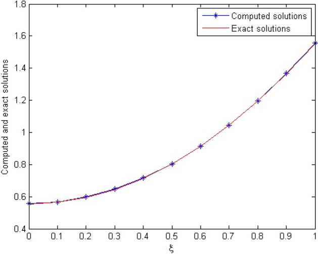
The comparison with the computed and exact solutions at $t=0.5$ with $\gamma =0.7$and $p=q=3$ for Problem 1.

Figure 4.

The contour plots of (a) computed solution. (b) exact solution, (c) the absolute error $p=q=4$ and $\gamma =0.5$ for Problem 1.

Table 1.

Absolute compared errors with $\gamma =0.5,t=0.5$ for Problem 1.

$\xi$	51	45	52	47	48	Our method
	$m=5,J=3$	$N_x=10,N_t=10$	$m=32$	$m=15,n=7$	$m=5$	$p=q=2$
0.1	6.481e−04	5.5127e−05	6.093e−03	7.964e−06	6.994e−05	1.4340e−10
0.2	4.109e−04	6.3034e−05	4.843e−03	1.721e−04	3.912e−06	1.8880e−10
0.3	5.493e−04	2.5286e−05	2.750e−02	2.472e−04	6.162e−06	2.1065e−10
0.4	5.198e−04	9.7841e−06	1.937e−02	2.912e−04	5.953e−06	2.0896e−10
0.5	4.912e−04	2.3230e−06	1.000e−06	3.004e−04	2.103e−06	1.8372e−10
0.6	5.063e−04	6.5798e−06	4.359e−02	2.760e−04	7.639e−06	1.3493e−10
0.7	5.045e−04	3.6040e−06	1.734e−02	2.213e−04	1.967e−06	6.2598e−11
0.8	5.040e−04	1.8435e−06	7.750e−02	1.440e−04	8.103e−06	3.3282e−11
0.9	5.037e−04	6.3126e−05	4.443e−02	5.026e−05	6.019e−06	1.5271e−10

Table 2.

Absolute errors for values of $p=q=2$, $p=q=3$ and $p=q=4$, $\gamma =0.5,$ $t=0.1$ for Problem 1.

$\xi$	$p=q=2$	$p=q=3$	$p=q=4$
0.1	1.0481e−10	2.4486e−11	2.7755e−17
0.2	2.7048e−10	2.0630e−13	1.3877e−16
0.3	4.0141e−10	8.7591e−11	5.5511e−17
0.4	4.9762e−10	2.0219e−10	1.6653e−16
0.5	5.5910e−10	3.0690e−10	1.1102e−16
0.6	5.8584e−10	3.6500e−10	0
0.7	5.7786e−10	3.3978e−10	0
0.8	5.3514e−10	1.9453e−10	1.1102e−16
0.9	4.5770e−10	1.0744e−10	0
Time(s)	4.1074	16.2225	72.5018

• Problem 2. Consider the following TFCDE⁵³:

$$\begin{array}{c}\hfill D_{\eta }^{\gamma }u(\xi ,t)+\xi {\displaystyle \frac{\partial u(\xi ,t)}{\partial \xi }}-{\displaystyle \frac{{\partial }^{2}u(\xi ,t)}{\partial {\xi }^2}}=r(\xi ,t),0\le \xi \le 1,0<t\le 1,\end{array}$$ 49

subjected to the initial condition

$$\begin{array}{c}\hfill u(\xi ,0)=\xi -{\xi }^3,\end{array}$$

and $u(\xi ,t)$ vanish is on bounders i.e.

$$\begin{array}{c}\hfill u(0,t)=u(1,t)=0,\end{array}$$

and

$$\begin{array}{c}\hfill r(\xi ,t)={\displaystyle \frac{\mathrm{\Gamma }(1+2\gamma )}{\mathrm{\Gamma }(1+\gamma )}}{t}^{\gamma }(\xi -{\xi }^3)+(1+t^{2\gamma })(7\xi -3{\xi }^3),\end{array}$$

exact solution is $u(\xi ,t)=(1+t^{2\gamma })(\xi -{\xi }^3)$.

The absolute errors are computed. The comparison of absolute errors of the proposed method with the method in⁵³ tabulated in the Table 3, shows that our method is more efficient and accurate. Actually our method for $p=q=3$ yields the solution of system of $4\times 4$ but in⁵³ for $k=4,M=1$ needs to solve a system of $48\times 21$. In Table 4, we report the absolute errors at $t=0.1$ for various $\gamma$ , $p=q=4$, and the run time of our method is tabulated to show the effectiveness of our method.

Table 3.

Absolute compared errors with $\gamma =0.7,t=0.5$ for Problem 2.

$\xi$	Our method	53	Our method	53
	$p=q=3$	$k=4,M=1$	$p=q=4$	$k=5,M=2$
0.1	1.5258 e−04	3.3203e−03	2.1877e−05	1.6340e−03
0.2	2.9665 e−04	6.4390e−03	4.2260e−05	3.1686e−03
0.3	4.2269 e−04	9.1546e−03	5.9644e−05	4.5045e−03
0.4	5.2117 e−04	1.1266e−02	7.2663e−05	5.5425e−03
0.5	5.8257 e−04	1.2571e−02	8.0089e−05	6.1836e−03
0.6	5.9737 e−04	1.2870e−02	8.0830e−05	6.3291e−03
0.7	5.5603 e−04	1.1961e−02	7.3936e−05	5.8808e−03
0.8	4.4904 e−04	9.6461e−03	5.8594e−05	4.7409e−03
0.9	2.6687 e−04	5.7250e−03	3.4127e−05	2.8126e−03

Table 4.

Absolute errors with $p=q=4,$ and various $\gamma$ at $t=0.1$ for Problem 2.

$\xi$	$\gamma =0.3$	$\gamma =0.7$	$\gamma =0.9$
0.1	2.5024e−04	8.0124e−05	3.9414e−05
0.2	4.8248e−04	1.5450 e−04	7.5995e−05
0.3	6.7876e−04	2.1739 e−04	1.0691 e−04
0.4	8.2331e−04	2.6376 e−04	1.2968 e−04
0.5	9.0260e−04	2.8926 e−04	1.4218 e−04
0.6	9.0526e−04	2.9022 e−04	1.4261 e−04
0.7	8.2216e−04	2.6370 e−04	1.2953 e−04
0.8	6.4637e−04	2.0742 e−04	1.0184 e−04
0.9	3.7316e−04	1.1981 e−04	5.8802e−05
Time(s)	38.7477	37.1628	35.3639

Figure 5a,b represent the computed and the exact solutions for $p=q=5$ with $\gamma =0.5$ and $\gamma =0.9$ respectively. We plot the graph of the exact solution, the computed solution, and absolute errors in solution for $p=q=5$ and $\gamma =0.9$. in Fig. 6a–c respectively. In Fig. 7a–c the contour plots of the computed solution, the exact solution and absolute errors are represented for $p=q=5$ with $\gamma =0.9$, respectively.

Figure 5.

(a) The computed solution with $p=q=3$ and $\gamma =0.5$ . (b) The computed solution with $p=q=3$ and $\gamma =0.9$ for Problem 2.

Figure 6.

(a) The exact solution. (b) The computed solution. (c) the absolute error $p=q=5$ and $\gamma =0.9$ for Problem 2.

Figure 7.

Contour plots of (a) computed solution. (b) Exact solution, (c) the absolute error $p=q=5$ and $\gamma =0.9$ for Problem 2.

Conclusion

An efficient, accurate spectral collocation method based on orthogonalized Bernoulli polynomials has been developed for time fractional convection-diffusion problems. Our approach contains operational matrices for approximate derivatives as well as fractional derivative. Operational matrices for derivatives are sparse having one sub-diagonal non-zero entries only, and for the fractional derivatives operational matrix is diagonal only. Due to these properties and using spectral methods convergence our presented method is spectral and fast with low computation cost. The comparing numerical results justifies the effectiveness and accuracy of our proposed scheme.

Author contributions

J.R.: phd supervisor, review and edit the manuscript. A.M.: computational study, write the main manuscript text. M.M.A.: review the manuscript.

Data availability

Te datasets used and/or analysed during the current study available from the corresponding author on reasonable request.

Competing interests

The authors declare no competing interests.

References

- 1.Biswas, K., Bohannan, G., Caponetto, R., Lopes, A. M. & Machado, J. A. T. Fractional-Order Devices (Springer, 2017).
- 2.Milici, C., Drăgănescu, G. & Machado, J. T. Introduction to Fractional Differential Equations Vol. 25 (Springer, 2018).
- 3.Herrmann, R. Fractional Calculus: An Introduction for Physicists (World Scientific, 2011).
- 4.Khan S, Sadia H, Haq S, Khan I. Time fractional Yang-Abdel-Cattani derivative in generalized MHD Casson fluid flow with heat source and chemical reaction. Sci. Rep. 2023;13:16494. doi: 10.1038/s41598-023-43630-9. [DOI] [PMC free article] [PubMed] [Google Scholar]
- 5.Shakeel M, et al. Construction of diverse water wave structures for coupled nonlinear fractional Drinfel’d-Sokolov-Wilson model with beta derivative and its modulus instability. Sci. Rep. 2023;13:17528. doi: 10.1038/s41598-023-44428-5. [DOI] [PMC free article] [PubMed] [Google Scholar]
- 6.Jesus IS, Tenreiro Machado JA, Boaventura Cunha J. Fractional electrical impedances in botanical elements. J. Vib. Control. 2008;14:1389–1402. doi: 10.1177/1077546307087442. [DOI] [Google Scholar]
- 7.Ahmadi N, Vahidi AR, Allahviranloo T. An efficient approach based on radial basis functions for solving stochastic fractional differential equations. Math. Sci. 2017;11:113–118. doi: 10.1007/s40096-017-0211-7. [DOI] [Google Scholar]
- 8.Permoon M, Rashidinia J, Parsa A, Haddadpou H, Salehi R. Numerical solution of time-fractional fourth-order reaction-diffusion model arising in composite environments. J. Mech. Sci. Technol. 2016;30:3001–3008. doi: 10.1007/s12206-016-0306-3. [DOI] [Google Scholar]
- 9.Irandoust-Pakchin S, Abdi-Mazraeh S, Fahimi-Khalilabad I. Higher order class of finite difference method for time-fractional Liouville-Caputo and space-Riesz fractional diffusion equation. Filomat. 2024;38:505–521. doi: 10.2298/FIL2402505I. [DOI] [Google Scholar]
- 10.Jangi Bahador N, Irandoust-Pakchin S, Abdi-Mazraeh S. Numerical treatment of time-fractional sub-diffusion equation using p-fractional linear multistep methods. Appl. Anal. 2023 doi: 10.1080/00036811.2023.2283131. [DOI] [Google Scholar]
- 11.Fahimi-khalilabad I, Irandoust-Pakchin S, Abdi-Mazraeh S. High-order finite difference method based on linear barycentric rational interpolation for Caputo type sub-diffusion equation. Math. Comput. Simul. 2022;199:60–80. doi: 10.1016/j.matcom.2022.03.008. [DOI] [Google Scholar]
- 12.Shen S, Liu F, Anh V. Numerical approximations and solution techniques for the space-time Riesz–Caputo fractional advection-diffusion equation. Numer. Algorithm. 2011;56:383–403. doi: 10.1007/s11075-010-9393-x. [DOI] [Google Scholar]
- 13.Yuste S, Acedo L. An explicit finite difference method and new von Neuman-type stability analysis for fractional diffusion equation. SIAM J. Numer. Anal. 2005;42:1862–1874. doi: 10.1137/030602666. [DOI] [Google Scholar]
- 14.Wang Q, et al. An efficient parallel algorithm for Caputo fractional reaction-diffusion equation with implicit finite-difference method. Adv. Differ. Equ. 2016;207:1–12. doi: 10.1186/s13662-016-0929-9. [DOI] [Google Scholar]
- 15.Yang Q, Liu F, Turner I. Numerical methods for fractional partial differential equations with Riesz space fractional derivatives. Appl. Math. Model. 2010;34:200–218. doi: 10.1016/j.apm.2009.04.006. [DOI] [Google Scholar]
- 16.Salehian M, Abdi-mazraeh S, Irandoust-pakchin S, Rafati N. Numerical solution of Fokker–Planck equation using the flatlet oblique multiwavelets. Int. J. Nonlinear Sci. 2012;13:387–395. [Google Scholar]
- 17.Irandoust-pakchin S, Dehghan M, Abdi-mazraeh S, Lakestani M. Numerical solution for a class of fractional convection-diffusion equations using the flatlet oblique multiwavelets. J. Vib. Control. 2014;20:913–924. doi: 10.1177/1077546312470473. [DOI] [Google Scholar]
- 18.Kargar Z, Saeedi H. B-spline wavelet operational method for numerical solution of time-space fractional partial differential equations. Int. J. Wavelets Multiresolut Inf. 2017;15:1750034. doi: 10.1142/S021969131750034. [DOI] [Google Scholar]
- 19.Rashidinia J, Eftekhari T, Maleknejad K. A novel operational vector for solving the general form of distributed order fractional differential equations in the time domain based on the second kind chebyshev wavelets. Numer. Algorithm. 2021;88:1617–1639. doi: 10.1007/s11075-021-01088-8. [DOI] [Google Scholar]
- 20.Soltani Sarvestani F, Heydar M, NiKnam A, Avazzadeh Z. A wavelet approach for the multi-term time fractional diffusion-wave equation. Int. J. Comput. Math. 2019;96:640–661. doi: 10.1080/00207160.2018.1458097. [DOI] [Google Scholar]
- 21.Ezz-Eldien S. On solving fractional logistic population models with applications. Comput. Appl. Math. 2018;37:6392–6409. doi: 10.1007/s40314-018-0693-4. [DOI] [Google Scholar]
- 22.Rashidinia J, Mohmedi E. Convergence analysis of tau scheme for the fractional reaction-diffusion equation. Eur. Phys. J. Plus. 2018;133:402–416. doi: 10.1140/EPJP/I2018-12200-2. [DOI] [Google Scholar]
- 23.Alsuyuti MM, Doha EH, Ezz-Eldien SS, Bayoumi BI, Baleanu D. Modified Galerkin algorithm for solving multitype fractional differential equations. Math. Methods Appl. Sci. 2019;42:1389–1412. doi: 10.1002/mma.5431. [DOI] [Google Scholar]
- 24.Zhang H, Jiang X, Zheng R. Chebyshev-Legendre spectral method and inverse problem analysis for the space fractional Benjamin-Bona-Mahony equation. Numer. Algorithm. 2020;84:513–536. doi: 10.1007/s11075-019-00767-x. [DOI] [Google Scholar]
- 25.Ezz-Eldien S, Doha E, Wang Y, Cai W. A numerical treatment of the two-dimensional multi-term time-fractional mixed sub-diffusion and diffusion-wave equation. Commun. Nonlinear Sci. Numer. Simul. 2020;91:105445. doi: 10.1080/00036811.2023.2283131. [DOI] [Google Scholar]
- 26.Alsuyuti M, Doha E, Ezz-Eldien S. Galerkin operational approach for multi-dimensions fractional differential equations. Commun. Nonlinear Sci. Numer. Simul. 2022;114:106608. doi: 10.1016/j.cnsns.2022.106608. [DOI] [Google Scholar]
- 27.Rashidinia J, Mohmedi E. Numerical solution for solving fractional parabolic partial differential equations. Comput. Methods Differ. Equ. 2022;10:121–143. doi: 10.22034/CMDE.2021.41150.1787. [DOI] [Google Scholar]
- 28.Alsuyuti MM, Doha EH, Ezz-Eldien SS. Numerical simulation for classes of one-and two-dimensional multi-term time-fractional diffusion and diffusion-wave equation based on shifted Jacobi Galerkin scheme. Math. Methods Appl. Sci. 2023 doi: 10.1002/mma.9659. [DOI] [Google Scholar]
- 29.Nikan O, Tenreiro Machado J, Avazzadeh Z, Jafari H. Numerical evaluation of fractional Tricomi-type model arising from physical problems of gas dynamics. J. Adv. Res. 2020;25:205–216. doi: 10.1016/j.jare.2020.06.018. [DOI] [PMC free article] [PubMed] [Google Scholar]
- 30.Nikan O, Tenreiro Machado J, Golbabai A. Numerical solution of time-fractional fourth-order reaction-diffusion model arising in composite environments. Appl. Math. Model. 2021;89:819–836. doi: 10.1016/j.apm.2020.07.021. [DOI] [Google Scholar]
- 31.Lai J, Liu F, Anh VV, Liu Q. A space-time finite element method for solving linear Riesz space fractional partial differential equations. Numer. Algorithm. 2021;88:499–520. doi: 10.1007/s11075-020-01047-9. [DOI] [Google Scholar]
- 32.Ezz-Eldien SS, Doha EH, Bhrawy AH, El-Kalaawy AA, Machado JT. A new operational approach for solving fractional variational problems depending on indefinite integrals. Commun. Nonlinear Sci. Numer. Simul. 2018;57:246–263. doi: 10.1016/j.cnsns.2017.08.026. [DOI] [Google Scholar]
- 33.Erfanifar R, Hajarian M, Sayevand K. A family of iterative methods to solve nonlinear problems with applications in fractional differential equations. Math. Methods Appl. Sci. 2023 doi: 10.1002/mma.9736. [DOI] [Google Scholar]
- 34.Erfanifar R, Sayevand K, Ghanbari N, Esmaeili H. A modified Chebyshev -weighted Crank–Nicolson method for analyzing fractional sub-diffusion equations. Numer. Methods Part. Differ. Equ. 2021 doi: 10.1002/num.22543. [DOI] [Google Scholar]
- 35.Chen J, Wang Y, Song M, Zhao R. Analyzing the decoupling relationship between marine economic growth and marine pollution in china. Ocean Eng. 2017;137:1–12. doi: 10.1016/j.oceaneng.2017.03.038. [DOI] [Google Scholar]
- 36.Lin L, Yang J, Zhang B, Zhang B, Zhu Y. Simplified numerical model of 3-d groundwater and solute transport at large scale area. J. Hydrodyn. 2010;22:319–328. doi: 10.1016/S1001-6058(09)60061-5. [DOI] [Google Scholar]
- 37.Li J, et al. Quantitative assessment of groundwater pollution intensity on typical contaminated sites in china using grey relational analysis and numerical simulation. Environ. Earth Sci. 2015;74:3955–3968. doi: 10.1007/s12665-014-3980-4. [DOI] [Google Scholar]
- 38.Qin R, et al. A GIS-based software for forecasting pollutant drift on coastal water surfaces using fractional Brownian motion: A case study on red tide drift. Environ. Model. Soft. 2017;92:252–260. doi: 10.1016/j.envsoft.2017.03.003. [DOI] [Google Scholar]
- 39.Mukherjee A, et al. Impact of sanitation and socioeconomy on groundwater fecal pollution and human health towards achieving sustainable development goals across India from ground-observations and satellite-derived nightlight. Sci. Rep. 2019;9:15193. doi: 10.1038/s41598-019-50875-w. [DOI] [PMC free article] [PubMed] [Google Scholar]
- 40.Wang X, Zhang L, Han C, Zhang Y, Zhuo J. Simulation study of oxytetracycline contamination remediation in groundwater circulation wells enhanced by nano-calcium peroxide and ozone. Sci. Rep. 2023;13:9136. doi: 10.1038/s41598-023-36310-1. [DOI] [PMC free article] [PubMed] [Google Scholar]
- 41.Sayevand K, Machado JT, Masti I. Analysis of dual Bernstein operators in the solution of the fractional convection-diffusion equation arising in underground water pollution. J. Comput. Appl. Math. 2022;399:113729. doi: 10.1016/j.cam.2021.113729. [DOI] [Google Scholar]
- 42.Chandrasekhar S. Stochastic problems in physics and astronomy. Rev. Mod. Phys. 1943 doi: 10.1103/RevModPhys.15.1. [DOI] [Google Scholar]
- 43.Baukal J. R., Gershtein, V. & Li, X. J. Computational Fluid Dynamics in Industrial Combustion (CRC Press, 2000).
- 44.Zhou F, Xu X. The third kind Chebyshev wavelets collocation method for solving the time-fractional convection diffusion equations with variable coefficients. Appl. Math. Comput. 2016;280:11–29. doi: 10.1016/j.amc.2016.01.029. [DOI] [Google Scholar]
- 45.Biazar J, Asadi M. Finite integration method with RBFS for solving time-fractional convection-diffusion equation with variable coefficients. Comput. Methods Differ. Equ. 2019;7:1–15. [Google Scholar]
- 46.Chen LJ, Li M, Xu Q. Sinc-Galerkin method for solving the time fractional convection-diffusion equation with variable coefficients. Adv. Differ. Equ. 2020;504:1–16. doi: 10.1186/s13662-020-02959-5. [DOI] [Google Scholar]
- 47.Saadatmandi A, Dehghan M, Azizi MR. The sinc-Legendre collocation method for a class of fractional convection-diffusion equations with variable coefficients. Commun. Nonlinear Sci. Numer. Simul. 2012;17:4125–4136. doi: 10.1016/j.cnsns.2012.03.003. [DOI] [Google Scholar]
- 48.Saw V, Kumar S. The Chebyshev collocation method for a class of time fractional convection-diffusion equation with variable coefficients. Math. Methods Appl. Sci. 2021;44:6666–6678. doi: 10.1002/mma.7215. [DOI] [Google Scholar]
- 49.Uddin M, Haq S. RBFS approximation method for time fractional partial differential equations. Commun. Nonlinear Sci. Numer. Simul. 2011;16:4208–4214. doi: 10.1016/j.cnsns.2011.03.021. [DOI] [Google Scholar]
- 50.Jiang Y, Ma J. High-order finite element methods for time-fractional partial differential equations. J. Comput. Appl. Math. 2011;235:3285–3290. doi: 10.1016/j.cam.2011.01.011. [DOI] [Google Scholar]
- 51.Adibmanesh L, Rashidinia J. Sinc and b-spline scaling functions for time-fractional convection-diffusion equations. J. King Saud Univ-Sci. 2021;33:101343. doi: 10.1016/j.jksus.2021.101343. [DOI] [Google Scholar]
- 52.Chen Y, Wu Y, Cui Y, Wang Z, Jin D. Wavelet method for a class of fractional convection-diffusion equation with variable coefficients. J. Comput. Sci. 2010;1:1–16. doi: 10.1016/j.jocs.2010.07.001. [DOI] [Google Scholar]
- 53.Zhu, Y., X., & Nie. On a collocation method for the time-fractional convection-diffusion equation with variable coefficients. arXiv preprint arXiv:1604.02112 (2016).
- 54.Yang, X.-J. General Fractional Derivatives Theory: Methods and Applications. Taylor and Francis Group Vol. 1 (CRC Press, 2019).
- 55.Napoli A. Solutions of linear second order initial value problems by using Bernoulli polynomials. Appl. Numer. Math. 2016;99:109–120. doi: 10.1016/j.apnum.2015.08.011. [DOI] [Google Scholar]
- 56.Bazm S. Bernoulli polynomials for the numerical solution of some classes of linear and nonlinear integral equations. J. Comput. Appl. Math. 2015;275:44–60. doi: 10.1016/j.cam.2014.07.018. [DOI] [Google Scholar]
- 57.Samadyar N, Mirzaee F. Orthonormal Bernoulli polynomials collocation approach for solving stochastic itô-volterra integral equations of abel type. Int. J. Numer. Model. 2019;1:1–14. doi: 10.1002/jnm.2688. [DOI] [Google Scholar]
- 58.Almeida, R., Tavares, D. & Torres, D. F. The Variable-order Fractional Calculus of Variations (Springer, 2019).
Associated Data
This section collects any data citations, data availability statements, or supplementary materials included in this article.
Data Availability Statement