In Situ Sampling of NOx Emissions from United States Natural Gas Flares Reveals Heavy-Tail Emission Characteristic

Abstract

Natural gas flaring is a common practice employed in many United States (U.S.) oil and gas regions to dispose of gas associated with oil production. Combustion of predominantly hydrocarbon gas results in the production of nitrogen oxides (NOx). Here, we present a large field data set of in situ sampling of real world flares, quantifying flaring NOx production in major U.S. oil production regions: the Bakken, Eagle Ford, and Permian. We find that a single emission factor does not capture the range of the observed NOx emission factors within these regions. For all three regions, the median emission factors fall within the range of four emission factors used by the Texas Commission for Environmental Quality. In the Bakken and Permian, the distribution of emission factors exhibits a heavy tail such that basin-average emission factors are 2–3 times larger than the value employed by the U.S. Environmental Protection Agency. Extrapolation to basin scale emissions using auxiliary satellite assessments of flare volumes indicates that NOx emissions from flares are skewed, with 20%–30% of the flares responsible for 80% of basin-wide flaring NOx emissions. Efforts to reduce flaring volume through alternative gas capture methods would have a larger impact on the NOx oil and gas budget than current inventories indicate.

Short abstract

NOx emission factors for United States natural gas flares exhibit heavy tails not captured using current inventory frameworks.

1. Introduction

Natural gas associated with the extraction of oil is commonly flared to dispose of the gas in a controlled manner. The flare’s combustion aims to destroy the mostly hydrocarbon waste gas, converting it to carbon dioxide (CO₂) and water (H₂O), thus reducing the safety concerns of the gas onsite, as well as its climate impacts. In addition to CO₂, unburned hydrocarbons (e.g., methane), nitrogen oxides (NOx = NO + NO₂), volatile organic compounds (VOCs), soot, and products of incomplete combustion (PICs) are released during the flaring process.¹ NOx is a highly reactive oxidizer that leads to the formation of tropospheric ozone under NOx-limited conditions, affecting both regional air quality and the climate.² The main sources of NOx are fuel combustion and agriculture soils, where the relative importance of each sector varies regionally.^3,4 Due to its health and environmental impacts, in the United States (U.S.), the Clean Air Act requires the U.S. Environmental Protection Agency (EPA) to set National Ambient Air Quality Standards (NAAQS) for NO₂, the most prevalent form of NOx.^5,6

In the U.S., studies have investigated NOx from the oil and gas sector, deploying bottom-up accounting methods as well as airborne, ground, and satellite measurements and found regionally elevated NOx attributable to oil and gas (O&G) activities.⁷⁻¹¹ Dix et al. estimated that 7% and 11% of NOx emissions in the Permian and Bakken were from flaring in 2015; however, the relative role was found to change depending on the stage of operation (i.e., drilling versus production).⁷ While flaring is not the only source of NOx in O&G regions, recent works aim to investigate the direct impact of flaring on local air quality and human health.¹²⁻¹⁵ On larger scales, temporal trends in flaring have been explored using various space-based data products. Gas volumes from flares observable from space are estimated across the globe using measurements from the Visible Infrared Imaging Radiometer Suite (VIIRS) instrument.^16,17 Using nitrogen dioxide (NO₂) as a proxy for NOx, flaring trends have also been investigated using satellite retrievals in regions such as the Artic,¹⁸ Mexico,¹⁹ and Russia.²⁰ Investigations into the relationships between flare performance and parameters such as flare design, fuel composition, and crosswinds have been mostly conducted in laboratory and test facilities.²¹⁻²⁷ Quantifying NOx flaring emission rates as part of a Texas Commission on Environmental Quality (TCEQ) 2010 study, Torres et al. measured NOx formation from industrial flares under low flow conditions (0.1%–0.25% of maximum flow), finding emission differences between steam and air-assisted flares.²⁴ More recently, Shaw et al. characterized flaring efficiencies and NOx emission ratios for 58 plumes from offshore facilities in the North Sea, with the largest from floating production and offloading vessels.²⁸

For regulatory purposes, NOx from flares is inventoried in the U.S. by the EPA using an emission factor (EF = 0.068 lb of NOx/10⁶ BTU) in conjunction with reported activity data (A = flow rate × heating value of flare gas). This emission factor value was derived in a 1983 EPA study of air- and steam-assisted flares.²¹ The TCEQ framework applies four emissions factors depending on the flare type and gas heating value, with values ranging from 0.0485 to 0.138 lb NOx/10⁶ Btu.²⁹ Overall, few assessments of the real-world operation of flares have been made due to the challenging nature of in situ sampling of installed flares and the geographical spread of flares across O&G regions.^28,30−33

The limited observational constraints on assumptions used to estimate the impacts of natural gas flares is one focus of the Flaring & Fossil Fuels: Uncovering Emissions & Losses (F³UEL) project. Through multiple measurement campaigns, F³UEL aims to quantify two under-sampled parts of the O&G sector: offshore emissions and real-world flare operation. Across three years, 2020–2022, we conducted multiple airborne campaigns to address these observational gaps. Offshore measurements were made in the Gulf of Mexico, Alaska, and California, representing the entire nation’s major offshore infrastructure. Examination of emissions in the Gulf of Mexico and their climate impact is the subject of a separate study.³⁴ To investigate U.S. flare performance, we sampled the combustion plumes of real-world flares in the major U.S. oil and gas basins responsible for more than 80% of national flaring volumes: Bakken, Eagle Ford, and Permian, as shown in Figure 1.

Figure 1.

U.S. Flaring Trends. (a) Flaring locations as seen by VIIRS (red triangles) and F³UEL airborne sampling locations (black circles). The domains of interest are indicated by the shaded boxes for the Bakken (purple), Eagle Ford (green), and Permian (yellow). (b) Flare volumes estimated from VIIRS observations for the three study regions for 2012 to 2020. Compared to the U.S. total flare volumes (black line), these three regions are responsible for the majority of US flaring activity and drive national trends. Domain definitions and annual VIIRS-based flare volumes are provided in Table S1.

The F³UEL airborne data set represents a large collection of in situ measurements of flare plumes, with more than 600 intercepts of plumes from an estimated 300 flares. In a separate analysis we explored flare performance in terms of total methane emissions using this airborne data set, finding that flares in the major U.S. O&G basins emit around 5 times more methane than the default flare methane destruction removal efficiency assumption of 98%, due to a combination of inefficient and unlit flares.³⁵ In comparison to unburned methane, NOx is produced through the flare’s combustion, and therefore, flare NOx production is determined by the performance of active flares. As a result, the occurrence of unlit flares does not contribute to NOx flaring emissions. Using in situ measurements of CO₂ and NOx, we estimate a NOx emission factor of each airborne intercept of a flare plume. The number of flare plume intercepts allows us to evaluate flare NOx production on the basin scale.

2. Materials and Methods

2.1. Airborne Sampling Methodology

We conducted two airborne campaigns focused on flaring, sampling the Eagle Ford and Permian in 2020 (August 25 through September 4) and the Bakken in 2021 (June 28 through July 15). Using a small aircraft (Scientific Aviation) equipped with high precision instrumentation, we measured CH₄, CO₂ (Picarro G2401-m), NO (ECOphysics 88 NOe), NO₂ (Teledyne T5000U), along with meteorological parameters such as wind speed and direction,³⁶ temperature, and relative humidity (Vaisala). To sample a geographically wide set of flares, we created an initial set of flares based on approximate locations from the VIIRS annual product.^16,17 For a given flight and depending on the meteorological conditions (e.g., wind direction), an initial subset of flares was targeted. As a supplement to this initial list, the aircraft team pursued additional flares they were able to identify during flight, resulting in a combination of targeted and opportunistic flare measurements which sampled the full range of flare temperatures and volumes observed by VIIRS at the basin levels (see Figure S4 in Plant et. al³⁵). Upon visual identification of the flare, the aircraft sampled downwind of the flare at low altitudes (typically 200–1000 m) using the flame as a guide, adjusting the altitude until a peak in CO₂ was observed downwind, indicating that the flare plume was intercepted. An example of a flare sampling flight track and the corresponding CO₂, NOx, and CH₄ time series is shown in Figure 2. Multiple downwind legs were attempted to increase the likelihood of intercepting the plume and to provide repeat sampling. If no plume was observed in real-time, the airborne team moved on to the next possible flare location. This approach represents a hybrid of previous airborne flare sampling methods previously presented in the literature^30,31 and provides straightforward attribution to the flare with a highly targeted flight path, as well as a sufficient data for analysis resulting from sampling a well-mixed combustion plume typically less than 2 km downwind.

Figure 2.

F³UEL airborne flare sampling. (a) Airborne sampling of a flare in the Permian on September 4, 2020, where the flight track is colored by the observed CO₂ concentration (ppm). White squares indicated locations in the CO₂ time series where the peak has been attributed to a flare. (b) Corresponding concentration time series (relative to the beginning of sampling start time for this site) for CO₂ (top), NOx (middle), and CH₄ (bottom), where red squares indicate flare peaks derived from the CO₂ signal.

To isolate the flare plumes in the airborne time series, we identify the peaks of CO₂ that are less than 10 s in duration, indicating that the source is nearby and that also surpass an amplitude threshold such that there is sufficient signal-to-noise to perform our analysis. Regional variability greater than the temporal scale of the narrow combustion peaks is removed by subtracting from the 1 s data a smoothed 10 s signal (calculated using a moving average filter). From this differential signal, CO₂ peaks are flagged and used to subset the corresponding time intervals of CH₄, NO, and NO₂. Further details about the peak finding algorithm and methane-focused analysis are presented in Plant et. al.³⁵ Due to frequent calibration of the NO₂ instrument and lower signal-to-noise of the NO and NO₂ measurements, our data set includes over 480 flare intercepts from which we characterize NOx production, compared to the 600 intercepts characterized for CH₄ destruction removal efficiency. The sampling statistics per basin are provided in Table S2. For the subsequent NOx analysis, we equate the response times of the three spectroscopic instruments, of which NO₂ is the slowest, with a moving average filter of 6 s applied to the CO₂ and NO time signals, where the length of the filter is chosen to maximize the correlation between CO₂ and NO with NO₂ across the flare intercepts. Intercepts of the flare combustion plumes after equating instrument response times are shown for the example in Figure 2b.

Our sampling approach prioritized the collection of population level statistics of flare performance at the basin scale, inherently capturing flares of varying infrastructure and operating conditions. Additionally, we sampled the flare plumes under varying conditions (e.g., atmospheric transport, aircraft altitude). Errors potentially exist for emission factors calculated for individual flare intercepts, and thus, it is more robust to interpret this data set as a population at the basin scale. Attribution to particular flare locations on the ground and their corresponding design, maintenance, etc. was not the focus of this work. Nevertheless, we investigate possible correlations of NOx flare production with potential drivers in auxiliary data sets^16,37 (see Supporting Information); however, this analysis does not yield explanatory root causes in part due to uncertainty in spatially linking the distinct data sets.

2.2. NOx Emission Factors

With simultaneous measurements of NOx and CO₂ in the flare combustion plumes, along with assumptions about the energy value of carbon in the gas, we estimate the NOx production of each flare plume intercept. Using in situ measurement of flare exhaust, we calculate NOx emissions factors (EF_NOx) following the formulization in Torres et al.²⁴ and the EPA²¹ and presented in eq 1

1

where NOx:CO₂ is the observed tracer:tracer relationship within the flare plume, X_C is the heating value of the carbon content in the flare gas, and MW is the molecular weight of NOx. We employ a Model II ranged major axis regression to characterize the relationship between NOx and CO₂ and allow for the presence of noise on each concentration signal.³⁸ Due to the lower signal-to-noise (SNR) of the NO and NO₂ signals compared to that of CO₂, we also require that the correlation of NO₂:CO₂ and NO:CO₂ are both greater than zero to remove spurious negative slopes. The statistics summarizing the observed NOx:CO₂ slopes by basin are provided in Table S3. An alternative approach to characterize NOx:CO₂ is using an enhancement ratio, which does not require a correlation filtering scheme; however, the choice of analysis method yields comparable results at the basin scale (see Figure S1).

The value of X_C depends on the chemical composition of the gas and is calculated as the carbon content of the gas mixture required to release 1 × 10⁶ Btu of heat. The exact gas composition burned by individual flares is not readily available. Instead, we assume gas compositions based on the basin-average CH₄ mole fraction reported in the Green House Gas Reporting Program (GHGRP), along with values reported in the literature to arrive at representative values for each basin.³⁹⁻⁴¹ While compositions can vary significantly, the impact to the heating value of the carbon in the waste gas is a fraction of a percent at the basin scale (see Figure S2). Our basin-specific assumptions and values are provided in Table 1. For each basin, we assume 10% of the flare gas is noncombustible (e.g., CO₂, N₂) in order to encompass CO₂ mole fractions reported to the GHGRP (see Figure S3). In the absence of more granular flare gas composition information, we use this conservative assumption in an effort to not overestimate gas heating values and subsequently flare emissions. We do not explicitly account for fuel-bound nitrogen that might remain after processes to remove hydrogen sulfide (H₂S) from the gas due to a lack of abundance data; however, the lower heating value of species such as ammonia would reduce the overall heating value of the flare gas if not already encompassed in our assumption of 10% noncombustibles.

Table 1. Basin-Specific Gas Composition Assumptions and Calculated Carbon Heat Content (X_C) and Overall Gas Mixture Net Heating Value.

		Hydrocarbon Mole Fraction (relative)
	Net Heating Value22, Btu/lb (Btu/scf)	Bakken	Eagle Ford	Permian
Methane	21,433 (910)	0.55	0.76	0.67
Ethane	20,295 (1630)	0.25	0.14	0.17
Propane	19,834 (2371)	0.15	0.05	0.11
Butane	19,976 (2977)	0.04	0.03	0.04
Pentane	19,322 (3679)	0.01	0.02	0.01
	–	3.21	3.11	3.16
a	–	45,117	38,180	41,429

^aAssumes 10% noncombustible gas by mole fraction (total gas = 10% noncombustible +90% Hydrocarbons).

The true molecular weight of NOx is not constant and rather depends on the percentage that is NO and NO₂. Most combustion sources initially emit in the form of NO, which rapidly transforms to NO₂ under ambient conditions. As a result, emission factors developed for inventory purposes typically report the molecular weight of NOx as 46 g/mol, the value for NO₂.²¹ We measure both NO and NO₂ in the flare plumes and can therefore calculate a molecular weight based on the observed NO:NO₂ for each intercept (see Figure S4). Emission factors using an observationally derived molecular weight for NOx are lower (by about 12%–16% depending on the basin) than those calculated using only NO₂ (see Table S4) due the linear relationship between NOx EF and molecular weight as shown in eq 1. Conclusions drawn in this work do not depend on the choice of molecular weight approach; however, depending on the application, one method may be more appropriate. Note that accounting for NOx in terms of moles instead of weight would eliminate this distinction. The results presented below correspond to emissions factors where the weight of NOx is that of NO₂ such that they characterize the source performance and are not dependent when during the dynamic conversion from NO to NO₂ we intercepted the flare plume.

2.3. Extrapolation to Basin-Level NOx Emissions

Using our observationally derived NOx emission factors, we estimate NOx flaring emissions following the methodology utilized in the Fuel-Based Oil and Gas (FOG) Inventory.^7,9 Based on the annual flare volumes provided by VIIRS (V_VIIRS) in billion cubic meters (Bcm),¹⁷ the NOx emission calculation, shown in eq 2, converts estimated volumes to NOx emissions (metric tons/year) using an assumed heating value (HV) for the gas and flare emission factor (EF_NOx). In the current version of FOG, HV is assumed to be 26,700 ± 14,000 Btu/m³ with EF_NOx assigned to 0.065 ± 0.038 lb NOx/10⁶ Btu (see section S2 of Francoer et al.⁹).

2

Our airborne data set produces distributions of NOx emission factors for each basin, providing an observation-based update to flaring NOx emissions calculated using eq 2. To apply our observed EF_NOx data set to the basin level, we randomly resample (with replacement) our emission factor estimates to apply them to the population of flare volumes in the annual 2020 VIIRS flare volume data set. Over 10,000 iterations of a nonparametric bootstrap analysis, we allow X_C (eq 1) and HV (eq 2) to vary by ±10% to introduce variability at the individual flare intercept level comparable to the spread of basin gas compositions assumptions (Table 1).

The emission estimate in eq 2 is also directly proportional to the assumed heating value of the flare gas. The particular composition of gas flared at each stack is not publicly available, and therefore, we aim to assume representative gas compositions for each basin. The gas produced in these three predominately oil regions is rich in other hydrocarbons, namely, ethane, propane, butane, and pentane,^40,41 increasing the heating value of the gas. Our assumed basin-specific gas compositions are provided in Table 1.

Extrapolation to the basin-scale using this resampling approach aims to incorporate uncertainty in the flare measurements, emission factor assumptions, and flare volume estimates in addition to temporal variability in flare performance. Volume estimates from VIIRS carry their own uncertainties,⁴² however, in aggregate have been shown to be robust for offshore infrastructure.⁴³ Onshore, VIIRS likely misses smaller flares that are more challenging to quantify from space. As such, in our calculation, total flare volumes have the potential to be biased low.

3. Results and Discussion

3.1. Skewed NOx Emission Factors

For each airborne intercept of a flare plume, we calculate the corresponding NOx emission factor, the distributions of which are shown for each basin in Figure 3. Also shown in Figure 3 are vertical dashed lines representing the emission factor used by the EPA (0.068 lb NOx/10⁶ Btu)¹ and the four values used by the TCEQ for steam-assisted flares (low heating value −0.068 lb NOx/MMBtu, high heating value −0.0485 lb NOx/MMBtu) and other flares, including air or unassisted flares (low heating value −0.0641 lb NOx/MMBtu, high heating value −0.138 lb NOx/MMBtu).²⁹ For this categorization, low Btu corresponds to waste gas with a neat heating value of 192–1000 Btu/scf, while high Btu is for >1000 Btu/scf. The composition of the gas in the O&G regions under investigation in this work have considerable percentages of higher molecular mass hydrocarbons,^40,41 resulting in high overall gas heating value (see Table 1).

Figure 3.

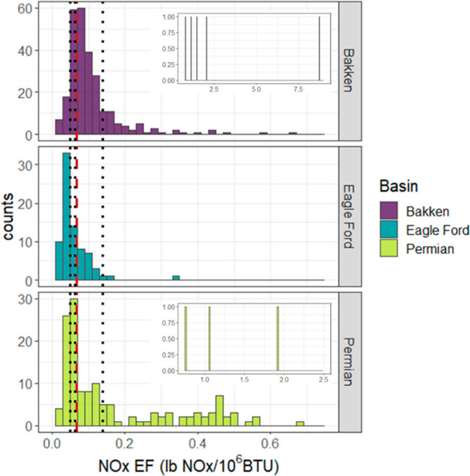
Estimated NOx emission factors for the Bakken (top, N = 268), Eagle Ford (middle, N = 78), and Permian (bottom, N = 140). The vertical dashed red line indicates the factor used by the EPA (0.068 lb NOx/10⁶ Btu), and the vertical dotted lines indicate the TCEQ values (0.0485, 0.0641, 0.068, 0.138 lb NOx/10⁶ Btu). Note that one TCEQ value overlaps with the EPA value and is not visible on the plot. For the Bakken and Permian, the occurrence of a few high emission factors is shown in the respective insets.

A summary of the estimated NOx emission factors is provided on the basin scale in Table 2. For the Bakken and Eagle Ford, the average emission factors observed are within the range of TCEQ emission factors. For the Permian, the mean emission factor observed is larger than the EPA and TCEQ values; however, the median value agrees better with TCEQ emission assumptions. An investigation into possible driving factors (Supporting Information) did not yield clear causes for variability in flare performance. The only statistically significant trends we observe are between emission factor and variability between multiple intercepts of the same flare for all basins and a negative correlation between the NOx emission factor and methane destruction removal efficiency in the Eagle Ford, both of which suggest the occurrence of suboptimal flare performance. The estimated emission factors are also consistent with a study of flaring in Norway,⁴⁴ which reported values of 1.16–2.36 g NOx/Sm³ (0.057–0.119 lb NOx/10⁶ BTU, assuming the American Petroleum Institute’s default gas heating value for unprocessed natural gas of 1235 BTU/scf⁴⁵). Our emissions factors are more comparable with air-assisted test flares sampled by Torres et al. (0.037–0.083 lb NOx/10⁶ BTU) compared to steam-assisted flares (0.009–0.033 lb NOx/10⁶ BTU) measured in that work.²⁴ Field measurements of NOx from flares in oil and gas production regions are limited; however, recent airborne measurements of 58 flare plumes in the North Sea found a mean NOx:CO₂ of 0.004 ppm/ppm (4 ppb/ppm),²⁸ which is considerably higher than our average observed signals, but within the range of our measurements (see Table S3). This difference in average value is possibly due to the high fractional methane content of the gas in their study region (median of 0.845) compared to our U.S. regions (Table 1), as well as the higher expected temperatures of these large offshore flares. In the Eagle Ford, our observed NOx:CO₂ slopes are consistent with combustion plumes attributed to flares in Roest and Schade (mean values of 0.33–1.47 ppb/ppm depending on the correlation and uncertainty thresholds).¹⁰ Both recent field studies found variability in observed flaring NOx emission ratios, with a general skewness toward higher values, consistent with the findings presented here.

Table 2. Observationally Derived NOx Emission Factors^a.

	Mean	Median	25th Quantile	75th Quantile	Minimum	Maximum	N
Bakken	0.159	0.086	0.064	0.123	0.011	8.74	268
Eagle Ford	0.060	0.049	0.034	0.073	0.011	0.334	78
Permian	0.194	0.102	0.052	0.295	0.020	1.92	140

^alb NOx/10⁶ Btu.

The spread in emission factors observed within a basin, and also between regions, suggests there is variability in flare NOx production that is not captured with a single emission factor. In the Eagle Ford, the average NOx emission factor is comparable to the EPA value,¹ while the Bakken and the Permian averages are closer to the largest TCEQ emission factor, assigned to air-assisted flaring of high heating value gas.²⁹ Within an individual basin we observe skewed distributions, particularly in the Bakken and Permian, such that a nontrivial number of flares we sampled were producing NOx at a factor of 2–5 greater than the largest emission factor used by the TCEQ for air flaring and unassisted flaring of high heating value gas. This heavy tail behavior has a direct impact to the air quality of regions downwind of the highest NOx emitting flares, and while not as densely populated as other regions in the country, an estimated 500,000 people live within 5 km of a flare in the Bakken, Eagle Ford, and Permian.⁴⁶

3.2. Basin-Level NOx Emissions Estimates

NOx flaring emissions, calculated using our observationally derived basin-specific emission factors and basin-specific heating value assumptions are compared to analogous emissions calculated using values employed by regulatory agencies and within the FOG inventory (Figure 4). For this comparison, the FOG inventory has been updated to incorporate 2020 and 2021 annual flaring volume inputs from VIIRS. Our analysis yields comparable flaring NOx emissions to those using the EPA and FOG assumptions for the Eagle Ford. For the Permian and Bakken, however, our emissions estimates are twice those based on EPA and FOG values. The majority of flare plumes we intercepted are within the range of emission factors employed by the TCEQ (0.0485–0.138 lb NOx/MMBtu²⁹); however, the heavy tail in the distributions observed in the Bakken and Permian (see Figure 2) result in basin-average emission factors (EF_NOx in eq 2) about 2–3 times larger than values employed by the EPA and FOG inventory.

Figure 4.

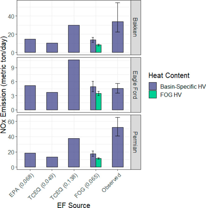
Basin-level flaring NOx emission estimates for 2020, comparing the influence of the assumed emissions factor (x-axis) and gas heating value (green: FOG value, 26,700 ± 14,000 Btu/m³; blue: basin-specific value used in this work, Table 1).

The assumed emission factor drives a large part of the discrepancy between our emission estimates and those of the FOG inventory for the Bakken and Permian; however, the assumed heating value of the gas (HV in eq 2) also contributes. The gas heating value in FOG is derived from the average of values from the U.S. Energy Information Administration (EIA) for the heating value of consumable natural gas (1037 Btu/ft³) and values in a study examining the performance of flares with low heating value gas (475 Btu/ft³).^24,47 The average of these two values results in a much lower assumed heating value (26,700 ± 14,000 Btu/m³, see Section S2 of Francoer et al.⁹) compared to our assumed values (see Table 1). There is limited publicly available gas composition data; however, our gas composition assumptions are chosen to be representative of the unprocessed gas in the high-flaring regions that are the focus of this work. Gas in these regions has a higher heating value due to the higher percentage of other hydrocarbons (ethane, propane, etc.) present in the associated gas.^40,41 The American Petroleum Institute (API) uses a standard of 1111 Btu/ft³ (39,200 Btu/m³) for the lower heating value of unprocessed or raw natural gas,⁴⁵ which is on the upper edge of the range used within FOG. Our assumptions are higher than this API standard, particularly in the Permian and Bakken (Table 1), due to the lower CH₄ gas content compared to the 81.6% assumed by the API. While our study does not provide new observational constraints on gas composition in these regions, we employ basin-specific assumptions derived from reported and literature values, which results in assumed heating values about 1.5 times those assumed in FOG.

Based on upward revisions to emissions factors and heating values for the Bakken and Permian, NOx emissions from flares using our estimated emission factors and assumed gas compositions are about 4 times larger than estimated in the FOG inventory in these regions. In the Eagle Ford, with the lowest observed emission factor, our estimates show good agreement with flaring emissions inventoried in FOG. Uncertainties exist in observational assessments of total NOx from these oil and gas regions.^7,9 Francoer et al. notes that emission factors used to calculate flaring emissions in FOG are based on available measurements of industrial flares, which may underestimate the NOx thermally produced by flares in O&G production regions by about a factor of 2.⁹ Our estimates support this underaccounting and indicate that for the Bakken and Permian flaring is responsible for a larger portion of the NOx emissions in these regions than represented in the FOG inventory.

4. Implications

The sensitivity of flaring NOx emission calculations to assumptions of emission factor and gas composition highlights a challenge bottom-up inventories face in accurately capturing the heterogeneity present in this sector of the O&G supply chain. The use of basin-specific emission factors and regional gas composition assumptions better capture average NOx flaring performance at the basin scale but would likely miss high emitters in the heavy tail of the skewed distributions. Given the wide range of estimated emission factors within a basin, employing a distribution of emission factors that encompasses high emitters would more accurately quantify the variability of real-world flare performance at the basin-scale.

Based on our estimates, flaring for these three regions in aggregate results in 90.5 t/day of NOx, which is <1% of the national estimate for total NOx emissions (21,578 t/day according to the NEI 2021⁴⁸). Undercounting for NOx from individual flares does therefore not have a large impact on the NOx budget at the national scale; however, very high NOx emitting flares are especially relevant for the assessments of air quality of the surrounding regions. In addition to workers in the area, an estimated 17.6 million people in the U.S. live within 1.6 km (∼1 mile) of active O&G wells.^49,50 In our study region, an estimated 500,000 people live within 5 km of a flare,⁴⁶ a distance that was found to be relevant for examining the impact of flaring on birth outcomes.⁵¹

Studies have shown that oil and gas emissions have degraded air quality in surrounding regions through increases in ozone concentrations, at times resulting in exceedances of EPA National Ambient Air Quality Standards (NAAQS).⁵²⁻⁵⁵ Pozzer et al. found that oil and gas emissions contributed to increased ozone in 90% of the contiguous U.S., with the highest summer enhancements seen in the central U.S., coincident with areas in nonattainment with ozone NAAQS.⁵² NOx is an important precursor of tropospheric ozone; however, the efficiency of its generation varies depending on other conditions (e.g., VOC/NOx ratio, solar radiance). In NOx-limited regions, such as Carlsbad Caverns National Park, NAAQS exceedances have been attributed to emissions, particularly NOx, from the nearby Permian basin.⁵³ In addition to the contribution to ozone generation, NOx also has a direct impact on air quality.^56,57 Buonocore et al. found that 2016 oil and gas emissions resulted in considerable health impacts (e.g., 410,000 asthma exacerbations), with NO₂ as the highest contributor to those adverse outcomes compared to ozone and PM2.5. They also found the influence of NO₂ was the most constrained spatially, while the influence of ozone was more dispersed, with the largest health impacts coincident with regions of high oil and gas activity (e.g., Texas).⁵⁷

Flares are not the only sources of NOx in oil and gas production regions. According to the source breakdown in the FOG inventory (see Table S6), flaring accounts for 23.6%, 4.2%, and 4.1% of total production NOx emissions in the Bakken, Eagle Ford, and Permian, respectively. Our flaring emissions estimate is comparable to the FOG inventory in Eagle Ford. In the Bakken, our estimate places flaring as the largest production source of NOx in the basin, assuming that all other sources are represented accurately in FOG. It is important to note that the FOG inventory does not include mobile sources. Underestimates of flaring in the Bakken could potentially explain some of the discrepancy between FOG and top-down estimates observed by Francouer et al.,⁹ although that comparison was made for 2015. In the Permian, our flaring estimate is comparable to accounting for artificial lift in FOG, behind emissions from wellhead compressors and drill rigs. While the precise attribution of NOx emissions to individual source categories in these oil and gas regions remains uncertain, source breakdowns in FOG used in conjunction with our flaring-specific estimate suggest that the reduction of flaring represents an opportunity for NOx reduction.

Extrapolation of the 2020 annual flare volume distribution observed by VIIRS to the basin scale (see Materials and Methods) using the EPA emission factor (0.068 lb NOx/10⁶ Btu) indicates that approximately 30%, 32%, and 35% of flares account for 80% of basin-wide flaring NOx emissions in the Permian, Bakken, and Eagle Ford, respectively. Applying our observationally derived emission factor increases the skew further with fewer flares accounting for more of the total emissions, with 80% of basin-wide flaring NOx emissions from approximately 19.2% (±1.2%; 1σ), 21.2 (±4.1%), and 29.7 (±1.3%) of flares in these regions. Our observation-based assessment of NOx production from flares suggests that efforts to reduce overall flaring volumes as well as those to identify and address the highest NOx emitting flares would have a larger air quality impact that was previously assumed using the default EPA assumptions.

Glossary

Abbreviations

NOx

nitrogen dioxides

BTU

British thermal unit

EF

emission factor

FOG

Fuel-Based Oil & Gas Inventory

VIIRS

Visible Infrared Imaging Radiometer Suite Nightfire product

Data Availability Statement

The airborne data presented in this work are available publicly on the University of Michigan Deep Blue Data Repository (2020 campaign: https://doi.org/10.7302/1xjm-3v49; 2021 campaign: https://doi.org/10.7302/6tgq-e116). Daily VIIRS data are available at https://eogdata.mines.edu/products/vnf/, and annual data are available at https://eogdata.mines.edu/download_global_flare.html. FOG flaring emissions updated with 2020 and 2021 VIIRS flaring volumes are at https://csl.noaa.gov/groups/csl7/measurements/2015songnex/emissions/.

Supporting Information Available

The Supporting Information is available free of charge at https://pubs.acs.org/doi/10.1021/acs.est.3c08095.

• Basin domain definitions, sensitivity analysis results, summary statistics of auxiliary data sets, and investigation into possible explanatory variables for flare performance (PDF)

Author Present Address

^⊥ Alan M. Gorchov Negron: Renewable and Sustainable Energy Institute, University of Colorado Boulder, Boulder, Colorado 80309, United States

Author Present Address

^# Graham Fordice: School for Environment and Sustainability, University of Michigan, Ann Arbor, Michigan 48109, United States

The authors declare no competing financial interest.

References

- United States Environmental Protection Agency . AP 42, Fifth Edition, Volume I Chapter 13: Miscellaneous Sources, Section 13.5 Industrial Flares, 2018. https://www.epa.gov/sites/default/files/2020-10/documents/13.5_industrial_flares.pdf (accessed 2022–01–11).
- Jacob D. J.Introduction to Atmospheric Chemistry; Princeton University Press, 1999. [Google Scholar]
- Almaraz M.; Bai E.; Wang C.; Trousdell J.; Conley S.; Faloona I.; Houlton B. Z. Agriculture Is a Major Source of NOx Pollution in California. Science Advances 2018, 4 (1), eaao3477 10.1126/sciadv.aao3477. [DOI] [PMC free article] [PubMed] [Google Scholar]
- Jaegle L.; Steinberger L.; Martin R. V.; Chance K. Global Partitioning of NO x Sources Using Satellite Observations: Relative Roles of Fossil Fuel Combustion, Biomass Burning and Soil Emissions. Faraday Discuss. 2005, 130 (0), 407–423. 10.1039/b502128f. [DOI] [PubMed] [Google Scholar]
- United States Environmental Protection Agency . Summary of the Clean Air Act. https://www.epa.gov/laws-regulations/summary-clean-air-act (accessed 2022–09–07).
- United States Environmental Protection Agency . Nitrogen Dioxide (NO2) Pollution. https://www.epa.gov/no2-pollution (accessed 2023–02–14).
- Dix B.; de Bruin J.; Roosenbrand E.; Vlemmix T.; Francoeur C.; Gorchov-Negron A.; McDonald B.; Zhizhin M.; Elvidge C.; Veefkind P.; Levelt P.; de Gouw J. Nitrogen Oxide Emissions from U.S. Oil and Gas Production: Recent Trends and Source Attribution. Geophys. Res. Lett. 2020, 47 (1), e2019GL085866 10.1029/2019GL085866. [DOI] [Google Scholar]
- Gorchov Negron A. M.; McDonald B. C.; McKeen S. A.; Peischl J.; Ahmadov R.; de Gouw J. A.; Frost G. J.; Hastings M. G.; Pollack I. B.; Ryerson T. B.; Thompson C.; Warneke C.; Trainer M. Development of a Fuel-Based Oil and Gas Inventory of Nitrogen Oxides Emissions. Environ. Sci. Technol. 2018, 52 (17), 10175–10185. 10.1021/acs.est.8b02245. [DOI] [PubMed] [Google Scholar]
- Francoeur C. B.; McDonald B. C.; Gilman J. B.; Zarzana K. J.; Dix B.; Brown S. S.; de Gouw J. A.; Frost G. J.; Li M.; McKeen S. A.; Peischl J.; Pollack I. B.; Ryerson T. B.; Thompson C.; Warneke C.; Trainer M. Quantifying Methane and Ozone Precursor Emissions from Oil and Gas Production Regions across the Contiguous US. Environ. Sci. Technol. 2021, 55 (13), 9129–9139. 10.1021/acs.est.0c07352. [DOI] [PubMed] [Google Scholar]
- Roest G. S.; Schade G. W. Air Quality Measurements in the Western Eagle Ford Shale. Elementa: Science of the Anthropocene 2020, 8 (18), na. 10.1525/elementa.414. [DOI] [Google Scholar]
- Ahmadov R.; McKeen S.; Trainer M.; Banta R.; Brewer A.; Brown S.; Edwards P. M.; de Gouw J. A.; Frost G. J.; Gilman J.; Helmig D.; Johnson B.; Karion A.; Koss A.; Langford A.; Lerner B.; Olson J.; Oltmans S.; Peischl J.; Pétron G.; Pichugina Y.; Roberts J. M.; Ryerson T.; Schnell R.; Senff C.; Sweeney C.; Thompson C.; Veres P. R.; Warneke C.; Wild R.; Williams E. J.; Yuan B.; Zamora R. Understanding High Wintertime Ozone Pollution Events in an Oil- and Natural Gas-Producing Region of the Western US. Atmospheric Chemistry and Physics 2015, 15 (1), 411–429. 10.5194/acp-15-411-2015. [DOI] [Google Scholar]
- Blundell W.; Kokoza A. Natural Gas Flaring, Respiratory Health, and Distributional Effects. Journal of Public Economics 2022, 208, 104601. 10.1016/j.jpubeco.2022.104601. [DOI] [Google Scholar]
- Fawole O. G.; Cai X.-M.; MacKenzie A. R. Gas Flaring and Resultant Air Pollution: A Review Focusing on Black Carbon. Environ. Pollut. 2016, 216, 182–197. 10.1016/j.envpol.2016.05.075. [DOI] [PubMed] [Google Scholar]
- Moneke A. N.; Ezeh C. C.; Obi C. J. Prevalence of Respiratory-Related Ailment among Residents of Gas Flaring States in Nigeria: A Systematic Review and Meta-Analysis. Air Qual Atmos Health 2022, 15, 1855. 10.1007/s11869-022-01221-z. [DOI] [Google Scholar]
- Willis M.; Hystad P.; Denham A.; Hill E. Natural Gas Development, Flaring Practices and Paediatric Asthma Hospitalizations in Texas. Int. J. Epidemiol 2021, 49 (6), 1883–1896. 10.1093/ije/dyaa115. [DOI] [PMC free article] [PubMed] [Google Scholar]
- Earth Observation Group . VIIRS Nightfire. https://eogdata.mines.edu/products/vnf/ (accessed 2022–02–08).
- Elvidge C. D.; Zhizhin M.; Baugh K.; Hsu F.-C.; Ghosh T. Methods for Global Survey of Natural Gas Flaring from Visible Infrared Imaging Radiometer Suite Data. Energies 2016, 9 (1), 14. 10.3390/en9010014. [DOI] [Google Scholar]
- Li C.; Hsu N. C.; Sayer A. M.; Krotkov N. A.; Fu J. S.; Lamsal L. N.; Lee J.; Tsay S.-C. Satellite Observation of Pollutant Emissions from Gas Flaring Activities near the Arctic. Atmos. Environ. 2016, 133, 1–11. 10.1016/j.atmosenv.2016.03.019. [DOI] [Google Scholar]
- Zhang Y.; Gautam R.; Zavala-Araiza D.; Jacob D. J.; Zhang R.; Zhu L.; Sheng J.-X.; Scarpelli T. Satellite-Observed Changes in Mexico’s Offshore Gas Flaring Activity Linked to Oil/Gas Regulations. Geophys. Res. Lett. 2019, 46 (3), 1879–1888. 10.1029/2018GL081145. [DOI] [Google Scholar]
- Ialongo I.; Stepanova N.; Hakkarainen J.; Virta H.; Gritsenko D. Satellite-Based Estimates of Nitrogen Oxide and Methane Emissions from Gas Flaring and Oil Production Activities in Sakha Republic, Russia. Atmospheric Environment: X 2021, 11, 100114. 10.1016/j.aeaoa.2021.100114. [DOI] [Google Scholar]
- McDaniel M.Flare Efficiency Study; U.S. Environmental Protection Agency, 1983.
- Johnson M. R.; Kostiuk L. W. A Parametric Model for the Efficiency of a Flare in Crosswind. Proceedings of the Combustion Institute 2002, 29 (2), 1943–1950. 10.1016/S1540-7489(02)80236-X. [DOI] [Google Scholar]
- Corbin D. J.; Johnson M. R. Detailed Expressions and Methodologies for Measuring Flare Combustion Efficiency, Species Emission Rates, and Associated Uncertainties. Ind. Eng. Chem. Res. 2014, 53 (49), 19359–19369. 10.1021/ie502914k. [DOI] [Google Scholar]
- Torres V. M.; Herndon S.; Wood E.; Al-Fadhli F. M.; Allen D. T. Emissions of Nitrogen Oxides from Flares Operating at Low Flow Conditions. Ind. Eng. Chem. Res. 2012, 51 (39), 12600–12605. 10.1021/ie300179x. [DOI] [Google Scholar]
- Pohl J. H.; Tichenor B. A.; Lee J.; Payne R. Combustion Efficiency of Flares. null 1986, 50 (4–6), 217–231. 10.1080/00102208608923934. [DOI] [Google Scholar]
- Seymour S. P.; Johnson M. R. Species Correlation Measurements in Turbulent Flare Plumes: Considerations for Field Measurements. Atmospheric Measurement Techniques 2021, 14, 5179–5197. 10.5194/amt-14-5179-2021. [DOI] [Google Scholar]
- Talebi A.; Fatehifar E.; Alizadeh R.; Kahforoushan D. The Estimation and Evaluation of New CO, CO2, and NOx Emission Factors for Gas Flares Using Pilot Scale Flare. Energy Sources, Part A: Recovery, Utilization, and Environmental Effects 2014, 36 (7), 719–726. 10.1080/15567036.2011.584117. [DOI] [Google Scholar]
- Shaw J. T.; Foulds A.; Wilde S.; Barker P.; Squires F. A.; Lee J.; Purvis R.; Burton R.; Colfescu I.; Mobbs S.; Cliff S.; Bauguitte S. J.-B.; Young S.; Schwietzke S.; Allen G. Flaring Efficiencies and NOx Emission Ratios Measured for Offshore Oil and Gas Facilities in the North Sea. Atmospheric Chemistry and Physics 2023, 23 (2), 1491–1509. 10.5194/acp-23-1491-2023. [DOI] [Google Scholar]
- Texas Commission on Environmental Quality . New Source Review (NSR) Emission Calculations, 2015. https://www.tceq.texas.gov/assets/public/permitting/air/Guidance/NewSourceReview/emiss_calc_flares.pdf.
- Gvakharia A.; Kort E. A.; Brandt A.; Peischl J.; Ryerson T. B.; Schwarz J. P.; Smith M. L.; Sweeney C. Methane, Black Carbon, and Ethane Emissions from Natural Gas Flares in the Bakken Shale, North Dakota. Environ. Sci. Technol. 2017, 51 (9), 5317–5325. 10.1021/acs.est.6b05183. [DOI] [PubMed] [Google Scholar]
- Caulton D. R.; Shepson P. B.; Cambaliza M. O. L.; McCabe D.; Baum E.; Stirm B. H. Methane Destruction Efficiency of Natural Gas Flares Associated with Shale Formation Wells. Environ. Sci. Technol. 2014, 48 (16), 9548–9554. 10.1021/es500511w. [DOI] [PubMed] [Google Scholar]
- Schwarz J. P.; Holloway J. S.; Katich J. M.; McKeen S.; Kort E. A.; Smith M. L.; Ryerson T. B.; Sweeney C.; Peischl J. Black Carbon Emissions from the Bakken Oil and Gas Development Region. Environ. Sci. Technol. Lett. 2015, 2 (10), 281–285. 10.1021/acs.estlett.5b00225. [DOI] [Google Scholar]
- Weyant C. L.; Shepson P. B.; Subramanian R.; Cambaliza M. O. L.; Heimburger A.; McCabe D.; Baum E.; Stirm B. H.; Bond T. C. Black Carbon Emissions from Associated Natural Gas Flaring. Environ. Sci. Technol. 2016, 50 (4), 2075–2081. 10.1021/acs.est.5b04712. [DOI] [PubMed] [Google Scholar]
- Gorchov Negron A. M.; Kort E. A.; Chen Y.; Brandt A. R.; Smith M. L.; Plant G.; Ayasse A. K.; Schwietzke S.; Zavala-Araiza D.; Hausman C.; Adames-Corraliza Á. F. Excess Methane Emissions from Shallow Water Platforms Elevate the Carbon Intensity of US Gulf of Mexico Oil and Gas Production. Proc. Natl. Acad. Sci. U. S. A. 2023, 120 (15), e2215275120 10.1073/pnas.2215275120. [DOI] [PMC free article] [PubMed] [Google Scholar]
- Plant G.; Kort E. A.; Brandt A. R.; Chen Y.; Fordice G.; Gorchov Negron A. M.; Schwietzke S.; Smith M.; Zavala-Araiza D. Inefficient and Unlit Natural Gas Flares Both Emit Large Quantities of Methane. Science 2022, 377 (6614), 1566–1571. 10.1126/science.abq0385. [DOI] [PubMed] [Google Scholar]
- Conley S. A.; Faloona I. C.; Lenschow D. H.; Karion A.; Sweeney C. A Low-Cost System for Measuring Horizontal Winds from Single-Engine Aircraft. Journal of Atmospheric and Oceanic Technology 2014, 31 (6), 1312–1320. 10.1175/JTECH-D-13-00143.1. [DOI] [Google Scholar]
- Drillinginfo, Inc. Drillinginfo Production Query, 2021. https://www.enverus.com/.
- Legendre P.Package “lmodel2. https://cran.r-project.org/web/packages/lmodel2/lmodel2.pdf (accessed 2022–09–12).
- United States Environmental Protection Agency . GHG Reporting Program Data Sets. https://www.epa.gov/ghgreporting/data-sets (accessed 2022–02–09).
- Brandt A. R.; Yeskoo T.; McNally M. S.; Vafi K.; Yeh S.; Cai H.; Wang M. Q. Energy Intensity and Greenhouse Gas Emissions from Tight Oil Production in the Bakken Formation. Energy Fuels 2016, 30 (11), 9613–9621. 10.1021/acs.energyfuels.6b01907. [DOI] [Google Scholar]
- Howard T.; Ferrara T. W.; Townsend-Small A. Sensor Transition Failure in the High Flow Sampler: Implications for Methane Emission Inventories of Natural Gas Infrastructure. J. Air Waste Manage. Assoc. 2015, 65 (7), 856–862. 10.1080/10962247.2015.1025925. [DOI] [PubMed] [Google Scholar]
- Schade G. W. Standardized Reporting Needed to Improve Accuracy of Flaring Data. Energies 2021, 14 (20), 6575. 10.3390/en14206575. [DOI] [Google Scholar]
- Brandt A. R. Accuracy of Satellite-Derived Estimates of Flaring Volume for Offshore Oil and Gas Operations in Nine Countries. Environ. Res. Commun. 2020, 2 (5), 051006. 10.1088/2515-7620/ab8e17. [DOI] [Google Scholar]
- Bakken J.; Langørgen Ø.; Husdal G.; Henriksen T. S.. Improving Accuracy in Calculating NOx Emissions from Gas Flaring. In SPE International Conference on Health, Safety, and Environment in Oil and Gas Exploration and Production, Nice, France, April 2008; Paper Number: SPE-111561-MS. 10.2118/111561-MS [DOI]
- American Petroleum Institute. Compendium of Greenhouse Gas Emission Methodologies for the Natural Gas and Oil Industry. https://www.api.org/-/media/Files/Policy/ESG/GHG/2021-API-GHG-Compendium-110921.pdf?la=en&hash=4B6E056EC663A4DE6133ED2A6F2F9865D7D33FA9 (accessed 2022–08–29).
- Cushing L. J.; Chau K.; Franklin M.; Johnston J. E. Up in Smoke: Characterizing the Population Exposed to Flaring from Unconventional Oil and Gas Development in the Contiguous US. Environ. Res. Lett. 2021, 16 (3), 034032. 10.1088/1748-9326/abd3d4. [DOI] [Google Scholar]
- Torres V. M.; Herndon S.; Kodesh Z.; Allen D. T. Industrial Flare Performance at Low Flow Conditions. 1. Study Overview. Ind. Eng. Chem. Res. 2012, 51 (39), 12559–12568. 10.1021/ie202674t. [DOI] [Google Scholar]
- United States Environmental Protection Agency . Criteria pollutants National Tier 1 for 1970 - 2022. Air Pollutant Emissions Trends Data. https://www.epa.gov/air-emissions-inventories/air-pollutant-emissions-trends-data (accessed 2023–06–29).
- Czolowski E. D.; Santoro R. L.; Srebotnjak T.; Shonkoff S. B. C. Toward Consistent Methodology to Quantify Populations in Proximity to Oil and Gas Development: A National Spatial Analysis and Review. Environ. Health Perspect 2017, 125 (8), 086004. 10.1289/EHP1535. [DOI] [PMC free article] [PubMed] [Google Scholar]
- Proville J.; Roberts K. A.; Peltz A.; Watkins L.; Trask E.; Wiersma D. The Demographic Characteristics of Populations Living near Oil and Gas Wells in the USA. Popul Environ 2022, 44, 1. 10.1007/s11111-022-00403-2. [DOI] [Google Scholar]
- Cushing L. J.; Vavra-Musser K.; Chau K.; Franklin M.; Johnston J. E. Flaring from Unconventional Oil and Gas Development and Birth Outcomes in the Eagle Ford Shale in South Texas. Environ. Health Perspect. 2020, 128 (7), 077003. 10.1289/EHP6394. [DOI] [PMC free article] [PubMed] [Google Scholar]
- Pozzer A.; Schultz M. G.; Helmig D. Impact of U.S. Oil and Natural Gas Emission Increases on Surface Ozone Is Most Pronounced in the Central United States. Environ. Sci. Technol. 2020, 54 (19), 12423–12433. 10.1021/acs.est.9b06983. [DOI] [PMC free article] [PubMed] [Google Scholar]
- Pollack I. B.; Pan D.; Marsavin A.; Cope E. J.; Juncosa Calahorrano J.; Naimie L.; Benedict K. B.; Sullivan A. P.; Zhou Y.; Sive B. C.; Prenni A. J.; Schichtel B. A.; Collett J.; Fischer E. V. Observations of Ozone, Acyl Peroxy Nitrates, and Their Precursors during Summer 2019 at Carlsbad Caverns National Park, New Mexico. J. Air Waste Manage. Assoc. 2023, 73, 951–968. 10.1080/10962247.2023.2271436. [DOI] [PubMed] [Google Scholar]
- Edwards P. M.; Brown S. S.; Roberts J. M.; Ahmadov R.; Banta R. M.; deGouw J. A.; Dubé W. P.; Field R. A.; Flynn J. H.; Gilman J. B.; Graus M.; Helmig D.; Koss A.; Langford A. O.; Lefer B. L.; Lerner B. M.; Li R.; Li S.-M.; McKeen S. A.; Murphy S. M.; Parrish D. D.; Senff C. J.; Soltis J.; Stutz J.; Sweeney C.; Thompson C. R.; Trainer M. K.; Tsai C.; Veres P. R.; Washenfelder R. A.; Warneke C.; Wild R. J.; Young C. J.; Yuan B.; Zamora R. High Winter Ozone Pollution from Carbonyl Photolysis in an Oil and Gas Basin. Nature 2014, 514 (7522), 351–354. 10.1038/nature13767. [DOI] [PubMed] [Google Scholar]
- Pacsi A. P.; Kimura Y.; McGaughey G.; McDonald-Buller E. C.; Allen D. T. Regional Ozone Impacts of Increased Natural Gas Use in the Texas Power Sector and Development in the Eagle Ford Shale. Environ. Sci. Technol. 2015, 49 (6), 3966–3973. 10.1021/es5055012. [DOI] [PubMed] [Google Scholar]
- Faustini A.; Rapp R.; Forastiere F. Nitrogen Dioxide and Mortality: Review and Meta-Analysis of Long-Term Studies. Eur. Respir. J. 2014, 44 (3), 744. 10.1183/09031936.00114713. [DOI] [PubMed] [Google Scholar]
- Buonocore J. J.; Reka S.; Yang D.; Chang C.; Roy A.; Thompson T.; Lyon D.; McVay R.; Michanowicz D.; Arunachalam S. Air Pollution and Health Impacts of Oil & Gas Production in the United States. Environmental Research: Health 2023, 1 (2), 021006. 10.1088/2752-5309/acc886. [DOI] [Google Scholar]
Associated Data
This section collects any data citations, data availability statements, or supplementary materials included in this article.
Supplementary Materials