Teacher Effects on Student Achievement and Height: A Cautionary Tale

Abstract

We apply “value-added” models to estimate the effects of teachers on an outcome they cannot plausibly affect: student height. When fitting commonly estimated models to New York City data, we find that the standard deviation of teacher effects on height is nearly as large as that for math and reading, raising potential concerns about value-added estimates of teacher effectiveness. We consider two explanations: non-random sorting of students to teachers and idiosyncratic classroom-level variation. We cannot rule out sorting on unobservables, but find students are not sorted to teachers based on lagged height. The correlation in teacher effects estimates on height across years and the correlation between teacher effects on height and teacher effects on achievement are insignificant. The large estimated “effects” for height appear to be driven by year-to-year classroom by teacher variation that is not often separable from true effects in models commonly estimated in practice. Reassuringly for use of these models in research settings, models which disentangle persistent effects from transient classroom-level variation yield the theoretically expected effects of zero for teacher value added on height.

1. Introduction

The increased availability of data linking students to teachers has made it possible to use various strategies to estimate the contribution teachers make to student achievement. By nearly all accounts, estimates of this contribution are large. Widely-reported estimates of the impact of a one standard deviation (σ) increase in teacher “value-added” on math and reading achievement typically range from 0.10 to 0.30σ, which suggest that a student assigned to a more effective teacher will experience nearly a year’s more learning than a student assigned to a less effective teacher (Hanushek & Rivkin 2010; Harris 2011; Jackson, Rockoff, & Staiger 2013; Koedel, Mihaly, & Rockoff 2015). These estimates—and evidence that teacher value-added measures (VAMs) are predictive of long-run outcomes (Chetty et al. 2014b)—provide the basis for the oft-cited assertion that teachers are the most important school input into student learning.

In addition to being used in research, several forms of VAMs are increasingly widely used in policy and practice. In these settings, in which VAMs may be used to make high-stakes decisions about teacher hiring, retention, or compensation (e.g., Dee & Wyckoff 2015; Mead 2012), it is desirable that the modeling strategies employed return teacher effectiveness estimates that are both unbiased and precise. However, prior research has raised important questions about the VAM modeling strategies for evaluating individual teachers (e.g., Baker et al. 2010; Braun, Chudowsky, & Koenig 2010). Because teachers are not randomly assigned to students, VAMs as estimated in observational data may be biased by student, classroom, or school influences on achievement that vary with teacher assignment (Dieterle et al. 2014; Kane 2017; Horvath 2015; Porvath & Amerein-Beardsley 2014; Rothstein 2010). Even if specific VAM modeling strategies return unbiased estimates, they may be imprecise if a large share of their variability is attributable to student and classroom-level error (McCaffrey et al. 2009; Schochet & Chiang 2013), and this issue may be more important for teachers with fewer students contributing to their estimates.

In this paper, we re-visit these questions of bias and precision in value-added modeling by estimating the effects of teachers on an individual-level outcome they cannot plausibly affect: student height. When fitting value-added models without classroom-by-teacher level error adjustments—a model specification that is often used to estimate annual value-added in educational practice—to data from 4^th and 5^th graders enrolled in New York City public schools between 2007 and 2010, we find that teacher “effects” on height are nearly as large as those on math and reading achievement. For instance, we find a 1σ increase in “value-added” on the height of New York City 4th graders is about 0.22σ, or 0.65 inches. This compares to 0.29σ and 0.26σ in math and English language arts, respectively. Moreover, the standard deviations of these teacher effects on height are statistically significant when measured using permutation tests. Models that control for school effects reduce the dispersion in effects on height, although the effects remain large and comparable to those on achievement at 0.16σ – 0.17σ.

On their face, findings of teacher effects on height raise concerns about what these models are capturing. We consider two possible explanations for this surprising rejection of the null that teachers do not affect height that we can test in our data. The first is that they reflect sorting, in which students differ systematically across teachers on unobserved factors related to height or changes in height. To the extent that these unobserved factors are also related to achievement or achievement gains, this finding might raise concerns of bias in VAMs for achievement. The second possible explanation is that non-zero estimates of teacher effects on height which do not account for year to year classroom-by-teacher shocks come about because student and/or classroom-level error (shocks) are improperly attributed to teachers, raising concerns about the precision and/or magnitude of VAM estimates. The appeal of using individually-measured height as an outcome is that we can explore these questions with real, as opposed to simulated, data in a setting in which true effects are implausible, we believe ex ante the null that effects should be zero, and where the outcome, height, is likely measured with less error than is student achievement.

We first consider bias due to sorting on height or unobservables correlated with height as an explanation for estimating non-zero teacher effects on height. We do this first by testing for systematic sorting of students within schools—which might indicate sorting on an unobserved variable—using a simple teacher fixed effects model to predict students’ prior-year outcomes. While more than 60% of NYC schools appear to track students to classrooms on prior achievement, we find little evidence of such sorting on height. Second, we estimate intertemporal correlations in teacher effects for height using multiple years of classroom data for each teacher. While this correlation across years for the same teachers is positive for achievement, the correlation for value added on height is close to zero, suggesting there is no systematic sorting of students to teachers on factors related to height gains across time, and no “persistent” effect on height. We also examine the correlation between teachers’ estimated effect on height and their effect on achievement. If height effects were to reflect sorting on unobservables that were related to achievement, one might expect these to be correlated. Instead, we find a correlation near zero.

We address the role of idiosyncratic or other variation in explaining “effects” of teachers on height in several ways. First, we perform a series of permutation tests that randomly allocate students to teachers without replacement in our data set and re-estimate each VAM model. This approach eliminates any potential for sorting, peer effects, systematic measurement error (e.g., at the classroom or school level), and/or true effects in the permuted data; it provides a benchmark for what teacher “effects” look like simply due to sampling variation in a model without classroom-level error adjustments (what we later refer to as a “2-level” model). Using this benchmark, we can reject the null hypothesis of a zero standard deviation in teacher effects on height (and on achievement), suggesting the presence of at least some systematic unexplained variation across teachers. Second, we estimate several variations of “3-level” models that are designed to disentangle the persistent component of teacher effects from transitory classroom shocks; one prominent implementation of this model uses the covariance in effects from successive years of teacher data to “shrink” estimated effects (Kane & Staiger 2008; Kane, Rockoff, & Staiger 2008; Chetty et al. 2014a). In our context, this is the only approach that results in the theoretically expected effects of zero for value added on height. These models estimate the persistent component of teacher contributions to height and achievement and thus by their nature do not estimate the year to year changes that could reflect teacher effort or negative shocks to teacher performance. Unfortunately, such models are not common in educational practice, raising the risk that transitory shocks are misinterpreted as signals of teacher effectiveness. These 3-level models are also limited in that they require multiple years of classroom data to estimate the cross-year correlation in teacher effectiveness, and teachers without multiple years of data are not used to estimate the shrinkage factor. The 3-level model also fails to capture real year-to-year differences in teacher effectiveness that are relevant for teacher evaluation, performance incentives, and professional development.

In the next section, we provide the framework for our analysis and ground our work in the context of a large literature on teacher value-added models. Then, in Sections 3 and 4 we describe our data sources and empirical approach. Section 5 presents our main results and a set of robustness checks, and Section 6 concludes with a discussion and lessons for researchers and policymakers.

2. Background: estimation and properties of VAMs

Teacher effects are defined as the systematic variation across teachers in student test performance that remains after accounting for the effects of other observed inputs, such as prior achievement, and economic or educational disadvantages. The most basic model is one like the following:

$$Y_{ijt}=\alpha Y_{ijt-1}+X_{ijt}^{\prime }\beta +u_{jt}+e_{ijt}.$$ (1)

In this model, Y_ijt and Y_ijt–1 are test scores for student i in classroom j in years t and t – 1, respectively, X_ijt is a vector of student-level covariates related to achievement (and potentially, teacher assignment), and u_jt is the teacher effect for teacher j in period t, modeled as either a fixed or random effect. e_ijt is a student-level error term. As written in (1), the same teacher may have different effects in different years; another implementation uses multiple years of student data to estimate a pooled effect for each teacher (u_j). The standard deviation in teacher effects (σ_u) is often interpreted as the variation in teacher quality, and ranges from 0.10 to 0.30σ, depending on model specification and setting, with effects usually larger in mathematics than in reading.¹

The use of VAMs in educational settings is controversial. For example, many oppose their use to evaluate individual teachers (e.g., American Statistical Association 2014). The most raised concern about VAMs is that they are biased; that is, that teacher effect estimates reflect systematic unmeasured student, school, or other inputs beyond the teacher’s control. A second concern is that they are noisy and imprecise; even if VAMs are unbiased, they are estimated from small samples and deviate from a teacher’s “true” effectiveness for idiosyncratic reasons. We briefly summarize the existing evidence on these concerns below.

2.1. Bias in VAMs for academic outcomes

A large literature has investigated whether and to what extent VAMs are biased. For example, a number of studies have asked whether model specification—the inclusion or exclusion of student or classroom controls, for example—affects VAM estimates (e.g., Ballou, Sanders, & Wright 2004; Ballou, Mokher, & Cavalluzzo 2012; Ehlert et al. 2013; Goldhaber, Goldschmidt, & Tseng 2013; Sass, Semykina, & Harris 2014; Kane et al. 2013). Apart from a control for prior achievement, these studies tend to find that the choice of covariates has only modest effects on the relative rankings of teachers. Rankings tend to be more sensitive to the inclusion of school fixed effects, which allow for systematic variation in achievement across schools due to sorting or other school-level inputs. Because school effects also absorb real differences in mean teacher effectiveness across schools, however, they are rarely used in practical applications such as school district estimates of teacher value added (Ehlert et al. 2014; Goldhaber, Walch, & Gabele 2013; Gordon, Kane, & Staiger 2006; Kane & Staiger 2008).

A more worrisome concern is that students are assigned to teachers on the basis of time-varying factors observed by schools but unobserved by the analyst. The available evidence on possible bias in VAMs due to non-random sorting is mixed. In a notable test of bias of this type, Rothstein (2010) showed that teachers assigned to students in the future had statistically significant “effects” on contemporaneous achievement gains when using several commonly-estimated VAM specifications with school fixed effects. Because such effects cannot be causal, Rothstein argued that these VAMs inadequately account for the process by which students are assigned to teachers.² However, Kane and Staiger (2008) randomly assigned teachers to classrooms within Los Angeles schools and found non-experimental VAM estimates were generally unbiased predictors of experimental VAMs, suggesting little bias (at least within schools in Los Angeles). This finding was replicated in the larger Measures of Effective Teaching (MET) project (Kane et al. 2013). Finally, a quasi-experimental study by Chetty et al. (2014a) that focused on teachers switching between schools found little evidence of bias compared to using all teachers (see also Bacher-Hicks, Kane, & Staiger 2014; Bacher-Hicks et al. 2017); although Rothstein (2017) and Chetty et al., (2017) differ in their views of the importance of any such bias.³ While these examples of randomization found consistency between VAM estimates in experimental or quasi experimental and non-experimental settings, outside of the randomized evaluations, we cannot be certain that these estimate the true effects of teachers. This suggests there is some benefit to applying commonly used VAMs to an outcome in which there is a strong prior expectation of a null effect.

2.2. Statistical imprecision and noise

Even if some specifications of VAMs are unbiased, their utility in evaluating individual teachers could be limited by statistical imprecision and instability, or “noise” (McCaffrey et al. 2009; Schochet & Chiang 2013). Imprecision stems not only from sampling error—a consequence of, for example, the small number of students used to estimate teacher effects—but also from classroom-level shocks and poor model fit, particularly for teachers with students in the tails of the distribution or with otherwise hard-to-predict achievement (Herrmann et al. 2016; Kane 2017). A practical implication of statistical imprecision is that annual VAM estimates vary from year to year, sometimes substantially, with within-teacher correlations ranging from 0.18 to 0.64, such that some seemingly effective teachers in one year are judged ineffective in the next, and vice versa.⁴

A common adjustment for imprecision in value-added estimates is Empirical Bayes shrinkage, which multiplies the VAM for each teacher by a shrinkage factor λ_j which ranges from zero to one (see Equation (2) below; Guarino et al. 2015; Hermann et al. 2016; Kane, Rockoff, & Staiger 2008; Koedel, Mihaly, & Rockoff 2015) and reflects the imprecision with which the teacher effects are measured. λ_j depends on n_j (the number of student observations for teacher j), and the overall fraction of variation in student achievement that is between as opposed to within teachers. Intuitively, a VAM estimate is “shrunk” toward the mean of zero when it is estimated with fewer students, or when the “signal” share of the variation in teacher effects is small.

Whether and how VAMs are “shrunk” depends in part on the structure and availability of data. Equation (1) above can be described as a “2-level” model, deployed in a setting in which teacher effects are estimated separately by year or multiple years of classroom data are pooled to improve precision in the estimation of a teacher effect (replacing u_jt with u_j). In both cases there are two dimensions of variation, between (${\sigma }_u^2$) and within (${\sigma }_e^2$) teachers, and the shrinkage factor is:

$${\lambda }_j=\frac{{\sigma }_u^2}{{\sigma }_u^2+\left({\sigma }_e^2/n_j\right)}$$ (2a)

With multiple years of classroom data, one can also estimate a “3-level” model, allowing for a classroom-level error component v_jt. In this case the shrinkage factor is:

$${\lambda }_j=\frac{{\sigma }_u^2}{{\sigma }_u^2+{\sigma }_v^2+\left({\sigma }_e^2/n_j\right)}$$ (2b)

where ${\sigma }_v^2$ is the within-teacher, between- classroom variance component. Importantly, v_jt is assumed to be idiosyncratic error uncorrelated with the “persistent” teacher effect u_j. In the 2-level model, however, real time-varying differences in teacher effectiveness cannot be separately identified from classroom-level shocks.⁵

Applications of value-added estimation models vary in whether they estimate annual teacher effects or effects pooled over years, whether they use shrinkage at all, whether they employ a 2- or 3-level model to separate “persistent” teacher effects from classroom shocks, and their procedure for estimating variance components (Guarino et al. 2015; Schochet & Chiang 2013). We describe these decisions in more detail in Section 4, where we discuss our analytic approach. For now, it is important to note that outside of research, the 3-level model is relatively rare. Multiple years of classroom data are not always available, and even when they are, policymakers and practitioners are often interested in annual measures of performance, rather than a time-invariant teacher effect (e.g., American Institutes for Research 2013; Isenberg & Hock 2010; VARC 2010).

3. Data

Our primary data source for estimating teacher effects on height and achievement is a panel of more than 360,000 students enrolled in grades 4–5 in New York City public schools between 2007 and 2010. These data are well-suited to our purposes, for several reasons. First, each student is linked to their mathematics and English Language Arts (ELA) teacher(s) and to annual measurements of their height from the city’s “Fitnessgram” physical fitness assessment. Second, the data represent a large population of students and teachers over four years. The number of students observed per teacher is large for some teachers, allowing for more precise estimates of teacher effects in 2-level models and for estimating 3-level models with multiple years of classroom data. Third, these data are typical of those used to estimate teacher VAMs in practice and were in fact used by the NYC Department of Education to evaluate teacher effectiveness in math and ELA (Rockoff et al., 2012). The Fitnessgram data include measures of student weight. We do not report results using weight in the interest of brevity, and because teachers may have real “effects” on weight (e.g., through their practices related to physical activity, such as recess participation and school meals/snacks) but are more unlikely to affect child height in the U.S. context.

We began with an administrative panel data set for students enrolled in grades 3–5 between 2005–06 and 2009–10. Among other things, this panel included student demographics (birth date, gender, race/ethnicity), program qualification and/or participation (Limited English Proficient, recent immigrant status, special education, and participation in the free and reduced school meals program—a measure of eligibility among those who apply for the program), and scaled scores in math and ELA, which we standardized by subject, grade, and year to mean zero and standard deviation one. These administrative data were matched to teacher-student linkages in math and ELA from 2006–07 to 2009–10.⁶ Third grade records and 2005–06 data were retained only to provide lagged values of the outcome measures.

The Fitnessgram has been conducted annually in NYC public schools since 2005–06 and relies on school staff—usually the physical education teacher—to measure students’ height, weight, and physical fitness. School personnel are trained to collect height and weight using a common procedure and a recommended digital beam scale.⁷ Measurements are taken throughout the school year, and the date of measurement is recorded in the Fitnessgram data. To parallel the estimation model and measures used in our achievement models, we standardized height by grade and year to mean zero and standard deviation one, with outlying values more than 4σ from the mean set to missing before standardization. We experimented with other methods for standardizing height, such as by gender and age in months. The reference group for standardization had little to no effect on our results. In all cases, we standardized using all available data, not the analytic sample, which was more restrictive. Our main results use standardized scores, but in one robustness check we used height gains measured in inches as the dependent variable (with no control for lagged height).

Descriptive statistics for students in our analytic sample are reported in Table 1, alongside statistics for the full population of students who could be linked to classroom teachers. Students in the analytic samples for height, math, and ELA were required to have a non-missing lagged dependent variable, non-missing covariates, and a teacher with seven or more students in the same grade with enough data to be included in the VAM models. Seven is a common minimum group size requirement used in other studies and in state teacher evaluation systems. For our baseline models which combine all four years of data, this minimum group size of 7 is not that restrictive. Table 1 shows the average 4th and 5th grader in our analytic sample was somewhat higher-achieving and smaller in stature than the full population of students linked to classroom teachers, with marginally higher ELA and math scores. The average 4th and 5th grader in NYC was 54.7 and 57.1 inches in height, respectively, with standard deviations of 3.0 and 3.2 inches. For later reference, the average 5th grader grew 2.5 inches between 4th and 5th grade, with a standard deviation of 1.8.

Table 1:

Mean student characteristics, analytic samples and all students

	Grade 4			Grade 5
	All linked obs.	Height sample	Math sample	All linked obs.	Height sample	Math sample
ELA z-score	0.027	0.072	0.051	0.025	0.069	0.047
Math z-score	0.033	0.103	0.079	0.035	0.119	0.087
Height (inches)	54.662	54.585	54.649	57.082	57.001	57.080
Height z-score	−0.008	−0.034	−0.012	−0.007	−0.031	−0.007
Female	0.506	0.509	0.507	0.505	0.507	0.507
White	0.156	0.169	0.162	0.152	0.167	0.157
Black	0.283	0.275	0.281	0.286	0.277	0.283
Hispanic	0.392	0.376	0.386	0.395	0.376	0.388
Asian	0.162	0.181	0.171	0.162	0.181	0.171
Age	9.645	9.626	9.640	10.670	10.646	10.665
Low income	0.798	0.804	0.804	0.799	0.805	0.806
LEP	0.119	0.102	0.105	0.101	0.082	0.086
Special ed	0.119	0.115	0.118	0.116	0.111	0.114
English at home	0.585	0.576	0.582	0.573	0.564	0.570
Recent immigrant	0.130	0.117	0.117	0.148	0.137	0.137
Same math/ELA teacher	0.900	0.883	0.893	0.862	0.858	0.867
Manhattan	0.133	0.119	0.125	0.131	0.115	0.125
Bronx	0.207	0.165	0.184	0.209	0.158	0.181
Brooklyn	0.312	0.340	0.325	0.310	0.348	0.328
Queens	0.284	0.302	0.299	0.287	0.304	0.299
Staten Island	0.064	0.074	0.068	0.063	0.074	0.068
2007	0.241	0.167	0.204	0.247	0.174	0.207
2008	0.243	0.225	0.241	0.244	0.235	0.242
2009	0.251	0.274	0.259	0.254	0.279	0.261
2010	0.264	0.334	0.297	0.255	0.311	0.290
N	239,577	153,242	182,623	236,983	143,738	180,639

Notes: “All linked observations” refers to all students who could be linked to their classroom teacher. The analytic samples include all students who meet the minimum data requirements to be included in the teacher value-added models for height or math. “Same math/ELA teacher” means the student has the same teacher code reported for math and ELA. In some cases, the teacher code differs because a teacher code is not reported for either math or ELA (more common for ELA, since not all students take this test). When conditioning on non-missing math and ELA teacher codes, the percent of 4th graders with the same math and ELA teacher code exceeds 98%; the percent of 5th graders exceeds 96%.

Table 2 reports the number of unique teachers and classrooms in our analytic samples, as well as descriptive statistics for the number of students per teacher (pooling all years) and per classroom (teacher-year). The full distributions are shown in supplemental appendix Figures A.1 and A.2. The analytic sample for the height analyses included approximately 4,300 4th grade teachers and 3,700 5^th grade teachers; the math analysis included 4,700 4^th grade teachers and 4,200 5^th grade teachers; the ELA analysis included 4,400 4^th grade teachers and 4,000 5^th grade teachers. Some teachers were observed with 80 or more students over four years, although the average teacher was observed for only two years with grade-subject means ranging from 36 to 42 students. The average number of students per classroom was 20–21 for all outcomes. Teachers in our math sample represent about 82–84 percent of all 4th-5th grade NYC teachers who could be linked to students during these years. Similarly, the teachers in our height and ELA samples represent 73–74 and 80–82 percent of all grade level teachers, respectively.

Table 2:

Count of unique teachers and classrooms, and students per teacher or classroom in analytic sample

	Height		Math		ELA
	Grade 4	Grade 5	Grade 4	Grade 5	Grade 4	Grade 5
Unique teachers (N)	4,263	3,687	4,721	4,249	4,366	3,978
Mean years observed	1.90	1.98	1.88	1.94	1.82	1.87
Students per teacher:
Mean	36.0	39.0	38.7	42.5	35.9	39.5
SD	22.9	25.5	24.5	27.4	22.8	24.9
p25	19	20	20	21	19	20
p50	27	29	29	33	26	29
p90	71	76	77	84	72	78
Unique classroom-years (N)	7,594	6,848	8,712	8,138	7,941	7,451
Students per classroom:
Mean	20.0	20.8	20.9	22.2	19.7	21.1
SD	5.4	6.4	5.1	6.4	5.6	6.3
p25	17	17	18	19	16	18
p50	20	21	21	22	20	21
p90	26	28	27	28	26	28

Notes: Teachers and classrooms are counted only when seven or more students were available with the minimum data to be included in the value-added models for these outcomes. For the full distributions, see the supplemental appendix.

Figures A.3 and A.4 in the supplemental appendix show histograms of student height and math achievement in the 4th and 5th grade analytic samples. For height, we show both the original measure in inches and the standardized measure. The distributions of both measures are roughly bell-shaped, although not normal: Kolmogorov-Smirnov tests reject normality, and there are a few low-scoring outliers in math. A small mass of students also scored at or near the test ceiling in math. We also benchmarked our height data to national norms, using CDC percentiles for height by sex and age (see Figure A.5 in the appendix). While students in our sample appear to be taller than the national norms—at all points in the distribution—year to year changes in height are comparable.

Table 3 reports pairwise correlations between student height, math, and ELA measures, between year-to-year changes in these measures, and between each measure and its lag. While the z-scores for math and ELA are strongly correlated (0.69 and 0.59 in 4th and 5th grade), achievement has only a weak bivariate correlation with height. The small negative correlation could be due to grade repeaters, who would be tall for their grade. In a multivariate regression model for achievement that includes height as a predictor with controls for lagged achievement, age, and other standard covariates, height is a statistically significant predictor of achievement in math and ELA for both grades 4 and 5. The implied effect size is small, however, with a 1σ increase in height associated with a 0.011σ to 0.015σ higher test score. See supplemental appendix Table A.1 for details. All three measures are strongly correlated with their lagged values, with correlations ranging from 0.65–0.68 in ELA and math to 0.79–0.80 in height. The intertemporal correlations in students’ height gains and in students’ achievement gains are very low.

Table 3:

Student-level bivariate correlations in outcome variables

Correlations between:	Grade 4	Grade 5
Math and ELA	0.688***	0.585***
Math and height	−0.059	−0.068***
ELA and height	−0.046***	−0.042***
Correlation with lag:	Grade 4	Grade 5
Math	0.701***	0.757***
ELA	0.683***	0.646***
Height	0.799***	0.793***
Correlations between changes in:	Grade 4	Grade 5
Math and ELA	0.158***	0.140***
Math and height	0.002	0.007**
ELA and height	0.013***	−0.006*

Notes: Pairwise correlations using all students with available data, not just those in the analytic VAM samples. All outcome measures are z-scores, where the height measure is standardized by grade and year. ***, **, and * indicate statistically significant correlations at the 0.0001, 0.01, and 0.05 levels, respectively.

4. Empirical methods

4.1. Value-added model specifications

For each grade level and outcome (math achievement, ELA achievement, and height) we estimated teacher effects using a standard “dynamic OLS” value-added regression model that conditions on the prior year’s outcome and a set of student-level covariates:

$$Y_{ijt}=\alpha Y_{ijt-1}+X_{it}^{\prime }\beta +{\gamma }_t+u_j+e_{ijt}$$ (3)

This model—in contrast to Equation (1)—pools all available years of classroom data for each teacher to estimate the teacher effect u_j. The covariates in X_it include a three-way interaction of gender, race, and age; recent immigrant status; limited English proficiency (LEP) and an indicator for a language other than English spoken at home; special education status; participation in free or reduced-price lunch (a measure of eligibility among those who apply for the program); and NYC borough of residence.⁸ γ_t is a year effect. We selected these covariates because they are commonly used in value-added models. The three-way interaction of gender, race, and age is atypical, but was thought to be appropriate in the model for height given variation in growth rates of children in this age range. Results are nearly identical with non-interacted controls. The height model includes an additional control for days elapsed between annual Fitnessgram measurements, the timing of which can vary between and within schools. We also estimated models including school fixed effects ϕ_s. While school effects are seldom used in practical applications, in our context height measurement or reporting practices could vary at the school level. The school fixed effect will absorb time-invariant effects of this type, but not time-varying differences.⁹

To represent the variety of ways in which teacher effects are estimated in practice, we estimated the u_j under both random and fixed effects assumptions.¹⁰ All of our estimates are shrinkage-adjusted, which we obtained using several alternative approaches. The first approach fit a random effects model using maximum likelihood and obtained the best linear unbiased predictor (BLUP) of each teacher effect, which is mathematically equivalent to an Empirical Bayes shrinkage estimate. The second approach fit a fixed effects model and then multiplied the estimated fixed effect by the shrinkage factor in (2) calculated using the variance components from this model. The third approach follows Kane, Rockoff, and Staiger (2008) and Chetty et al. (2014a) by estimating Equation 3 without teacher effects and calculating the mean residual for each teacher. Each teacher mean was then multiplied by the shrinkage factor λ_j.

As shown in Equations 2a–2b, the shrinkage factor differs for 2- and 3-level models. In a 2-level model with teacher and student variance components, teachers are observationally equivalent to a large classroom and ${\sigma }_u^2$ is the between-teacher variance. In a 3-level model with teacher, classroom, and student error components, there is an idiosyncratic classroom error with variance ${\sigma }_v^2$. These variance components can be estimated directly in a maximum likelihood model. Kane, Rockoff, and Staiger (2008) use a different approach and estimate between-teacher variance (${\sigma }_u^2$) as the covariance between estimated classroom effects ${\widehat{u}}_{jt}$ for the same teacher in successive years, for teachers with multiple years of data. Between-classroom variance ${\sigma }_v^2$ is estimated using the total variance in the residuals less the withinclassroom and between-teacher components. The “drift” model used by Chetty et al. (2014a, b) is like this approach in that it uses covariance in mean residuals across classrooms to estimate the between-teacher variance. The main difference is that the drift model does not assume a fixed correlation between two classroom years; the correlation in annual teacher effects weakens as time between measurements increases. We report results using all of these varied approaches.

4.2. Testing for sorting on prior characteristics

To assess the extent to which students are non-randomly sorted to classrooms within schools on prior characteristics, including height, we followed the approach used in Horvath (2015).¹¹ We identify schools with seemingly non-random sorting by height or achievement by testing for systematic variation in lagged student characteristics across classrooms within schools, grades, and years. For example, for each school s the following regression is estimated for the lagged outcome $Y_{it-1}$:

$$Y_{ijt-1}=u_{jt}+{\varphi }_{gt}+w_{ijt}$$ (4)

The $u_{jt}$ are teacher effects for year t and ϕ_gt are grade-year effects. Schools in which the null hypothesis of no systematic differences across classrooms is rejected are presumed to exhibit sorting on dimensions associated with their lagged value of $Y_{it}\left(H_0:u_{jt}=0\forall jt\right)$.

Schools may exhibit non-random sorting of students within grades and years, but not persistently “match” groups of students to specific teachers over time. To test for persistent teacher matching, we further regress mean lagged outcomes on school-grade-year indicators and teacher, rather than classroom dummies. Schools in which the null hypothesis of no teacher matching is rejected (the teacher dummies are jointly zero) are presumed to persistently match students to teachers.

Using this method, Horvath (2015) found more than half of all schools in North Carolina exhibited sorting within grade and year on prior achievement. Additionally, she found a somewhat smaller share appeared to actively balance the gender and race composition of classrooms, and a larger share exhibited within-school sorting by parental education. Moreover, she found roughly 40% of North Carolina schools persistently matched similar students to teachers across years. While not a definitive test for omitted variables bias, in our case this exercise sheds light on whether classrooms within schools are grouped on height (and thus possibly unobserved factors related to height) that might explain teacher effects on this outcome.

4.3. Permutation tests

To provide a benchmark for what the 2-level teacher “effects” look like in our data due to sampling variation, we performed permutation tests. For these tests, we randomly allocated students to teachers in our data set within grade and year, without replacement, and re-estimated each model. This random permutation was repeated 499 times, maintaining the actual number of students assigned to each teacher in each permutation. On each iteration, we saved the estimated standard deviation of teacher effects (${\widehat{\sigma }}_u$) and then examined the distribution of these estimates across all 499 iterations.¹²

These results were used as a Fisher exact randomization test to assess whether our estimates of the dispersion in teacher effects in the observed data differ from what one would expect under the null of no effects. Through randomization of students to teachers in our data, we effectively impose the null hypothesis of no sorting, no true teacher effect, no peer effects, and no systematic measurement error. If the estimated standard deviation from the observed data is larger than the 95^th percentile of standard deviations from the permutations, we conclude that the standard deviation is statistically different from the null of zero.¹³

5. Results

5.1. Teacher effects on achievement and height

Our estimates of various specifications for models of teacher effects on the achievement and height of 4th and 5th graders in NYC are summarized in Table 4. Each cell represents the estimated standard deviation of teacher effects for a given outcome, grade, and value-added model specification. We organize this table into “2-level” and “3-level” models, where the latter allow for an idiosyncratic classroom effect. We focus first on the 2-level models, as they are the most common, and later turn to the 3-level models. As explained previously, random effects estimates are either best linear unbiased predictors from a maximum likelihood random effects model (MLE) or shrinkage-adjusted mean residuals following Kane, Rockoff, and Staiger (KRS) or the Chetty et al. (2014a) drift model, as indicated in the table. For comparison, fixed effects estimates have also been shrinkage-adjusted.

Table 4:

Standard deviation of Bayesian shrunken estimated teacher effects

	Grade 4			Grade 5
Model specification:	Height	Math	ELA	Height	Math	ELA
A. 2-level models
RE	0.218	0.286	0.256	0.210	0.253	0.210
FE (shrunk)	0.250	0.344	0.278	0.315	0.258	0.240
RE w/school effects	0.169	0.216	0.184	0.157	0.199	0.155
FE w/school effects (shrunk)	0.166	0.202	0.172	0.160	0.189	0.145
Permutations: FE (mean ${\widehat{\sigma }}_u$ shown)	0.056	0.063	0.065	0.053	0.056	0.068
Permutations within school: FE	0.131	0.083	0.077	0.123	0.084	0.072
B. 3-level models
RE (KRS)	0.000	0.163	0.104	0.000	0.132	0.097
RE w/school effects (KRS)	0.000	0.107	0.077	0.002	0.087	0.062
RE (MLE)	0.000	0.199	0.159	0.000	0.164	0.121
RE w/school effects (MLE)	0.000	0.108	0.070	0.000	0.089	0.056
Chetty et al. drift model (RE)	0.057	0.180	0.128	0.031	0.143	0.123

Notes: For Panel A (2-level models), teacher effects were estimated in four ways: (1) assuming random teacher effects; (2) assuming fixed teacher effects and “shrinking” using the estimated signal-to-noise ratio after estimation; (3) assuming random teacher effects and including school fixed effects; and (4) assuming fixed teacher effects (shrunken after estimation) and including school effects—uses a two-stage method that regresses the outcome on covariates and school fixed effects and then uses the residuals to estimate the teacher fixed effects. For the random permutations we report the mean estimated standard deviation across 499 permutations of students to teachers. For Panel B (3-level models), we used the shrunken residual method from Kane, Rockoff, and Staiger (2008; KRS), or a random effects model with both teacher and classroom variance components (MLE). The last line of Panel B reports the standard deviation in best linear predictors from the teacher effects model with drift used in Chetty et al. (2014a).

The standard deviations of teacher effects on math and ELA achievement reported in Table 4 are largely consistent with those estimated elsewhere in the research literature. Beginning with the 2-level model reported in the first two rows of Table 4, we find a 1σ increase in teacher value-added to be associated with a 0.29σ – 0.34σ and 0.25σ – 0.26σ increase in math achievement for 4th and 5th graders, respectively. In ELA, the variation in effects is closer to 0.26σ – 0.28σ in 4th grade and 0.21σ – 0.24σ in 5th grade. These estimates are on the upper end of the range of those found in other studies, but close to those estimated by others using NYC data (e.g., Rockoff et al., 2012).

The standard deviations of teacher effects on height are smaller, but not substantially different in standard deviation units, from those estimated for mathematics and ELA achievement. We find the standard deviation of teacher effects on height is substantial in NYC. For instance, a 1σ increase in teachers’ “value-added” on height is associated with a 0.21σ – 0.22σ increase in height in the random effects model. The shrinkage-adjusted fixed effects yield somewhat larger values, from 0.25σ in 4th grade to 0.32σ in 5th grade. In every case, a test of the null hypothesis that the teacher effects are jointly zero is soundly rejected at any conventional level. To put these effects in perspective, a 0.22σ increase in height amounts to a 0.68-inch gain in stature for 4th graders and an 0.72-inch gain for 5th graders. This is roughly a third of a standard deviation in year-to-year growth for children of this age.

Figure 1 provides full pictures of the distribution of teacher effects on height and mathematics from the 2-level random and fixed effects models (see supplemental appendix Figure A.6 for ELA). Both distributions are approximately symmetric around zero, and there is generally less dispersion visible in the effects on height than in the effects on math. Comparing the 10th, 25th, 75th, and 90th percentiles of random effects in 4th grade, the centiles of teacher effects on height tend to be closer to zero (−0.22, −0.10, +0.10, and +0.21) than the same centiles for math (−0.31, −0.19, +0.15, and +0.34). The distribution of height effects is somewhat left-skewed, and the distribution of math effects somewhat right-skewed. There are a handful of relatively extreme values (>1.5σ) in the distribution of height effects—more so than in the distribution of math effects—but fewer than 10 in total (out of 4,262 teachers). Recall that a small number of students with outlier values for height were omitted from the analytic sample. The standard deviation of teacher effects on height, therefore, does not appear to be inflated by influential outliers.

Figure 1:

Distribution of teacher effects on height and math scores

Notes: See notes to Table 4 for a description of how teacher effects were estimated. N=4,262 4^th grade teachers and 3,687 5^th grade teachers.

The next two rows of Table 4 report similar estimates of dispersion in teacher effects for models with school effects. The inclusion of school effects should account for systematic differences in height across teachers due to school-level factors, such as (time-invariant) differences in Fitnessgram timing, practices for carrying out or reporting height measurements, and the like. In these cases, the estimated standard deviations are approximately 70–75 percent of those estimated in models without school effects. In all cases, however, the apparent effect of variations in teacher effects on height remains meaningful in magnitude, ranging from 0.16σ to 0.17σ. Standard deviations of teacher effects on math and ELA are comparably reduced when including school effects (to 0.15σ – 0.22σ).

Table A.5 in the supplemental appendix shows the estimated standard deviation of teacher effects on height from various alternative specifications of the 2-level models. These include models with higher polynomials in lagged height, models interacting student demographics (sex, race, and age) with lagged height, and models excluding the elapsed days between Fitnessgram measures. The results are all very similar to those in Table 4. Thanks to a referee suggestion, we also estimated regressions in which the year-to-year height gain (in inches) was used as the dependent variable, rather than the traditional dynamic OLS specification from Equation (3). This model is arguably more defensible for height, given its ratio scale, than for achievement. While the units are not directly comparable, we found comparably large teacher effects on height using this model.

In the supplemental appendix, we additionally report the results of an analysis using the nationally representative Early Childhood Longitudinal Survey – Kindergarten Cohort, 1998 (ECLS-K). These results are informative in that they show our findings of significant effects of 2-level value added models on height are present and significant using a national sample of students at a different age where the measurement of height was more careful. The ECLS-K drew a sample of kindergarteners in sampled schools; measured their achievement and height in the fall of their kindergarten year and again in the Fall of 1^st grade; and linked sampled students to their classroom teachers. The ECLS-K offers some advantages to the NYC data, including standardized height measurement by trained assessors and a richer set of covariates as well as nationally representative data. Further, there are fewer opportunities for dynamic sorting of students into classrooms in the ECLS-K data since this study begins with kindergarteners. As reported in Appendix Table B.1, we find a similar pattern of teacher effects on height and achievement in the ECLS-K data, indicating that our findings are not an artifact of the NYC public schools setting or Fitnessgram measurement protocols and practices.

5.2. Do teacher effects on height reflect sorting?

The results from Panel A of Table 4 indicate that the most commonly-estimated 2-level value-added models yield significant and implausible “effects” of teachers on height. A possible explanation is non-random sorting of students to teachers on unobserved factors related to height, or changes in height. These factors might include, for example, student health, ethnicity or immigration history, age (which can vary within grade with student age at kindergarten entry and grade retention history), or birthweight. If these unobserved factors are also related to achievement, this would be potentially troubling for achievement VAMs. That is, this is a possible problem if commonly used covariates in value-added models for achievement inadequately account for the effects of this sorting.

To explore this possibility, we first examined how teachers’ estimated effects on achievement correlate with their effects on height. These correlations are reported in Table 5 for the 2-level random and fixed effects models. There is little or no evidence of an association between teacher effects on height and academic achievement. In both 4th and 5th grade, we find the correlation between value-added on height and achievement is typically smaller than 0.05 in absolute value. We found similar results when using Spearman rank correlations. In contrast, the correlation between teachers’ value-added on math and ELA achievement is modest to strong, at 0.64–0.70 in 4th grade, and 0.51–0.56 in 5th grade. There were only two significant correlations between effects on height and achievement: the positive correlations of 0.199 and 0.090 between height and math effects in 4th and 5th grades, respectively. Both emerge only when teacher effects are estimated as fixed effects with shrinkage (and excluding school fixed effects); the corresponding correlations for random effects are close to zero. We have examined these two cases closely and have been unable to identify alternative explanations for these associations. For example, there are no outlier fixed effect estimates that drive up the correlation. The correlation is also not attributable to the shrinkage factor applied to the fixed effect estimates; the correlation is present before the adjustment. While not shown in this table, we also found similarly positive correlations between value-added on height and ELA in the fixed effects model, though these correlations are smaller than the correlation between math and height in this model.

Table 5:

Pairwise correlations between teacher effects

	Math VAM:
Grade 4:	RE	FE (adj)	RE w/school effects	FE w/school effects
Height VAM:
RE	−0.019	−0.014	−0.007	−0.008
FE (adj.)	−0.030+	0.199 *	−0.022	−0.023
RE w/school effects	0.000	−0.003	0.002	0.002
FE w/school effects (adj.)	−0.002	−0.004	0.001	0.000
ELA VAM:
RE	0.697 *	0.597*	0.521*	0.519*
FE (adj.)	0.658*	0.689 *	0.477*	0.475*
RE w/school effects	0.525*	0.432*	0.646 *	0.643*
FE w/school effects (adj.)	0.522*	0.428*	0.643*	0.641 *
Grade 5:	RE	FE (adj)	RE w/school effects	FE w/school effects
Height VAM:
RE	0.016	0.015	0.002	0.002
FE (adj.)	0.009	0.090 *	0.005	0.005
RE w/school effects	0.001	0.002	−0.006	−0.007
FE w/school effects (adj.)	0.000	0.002	0.005	0.005
ELA VAM:
RE	0.557 *	0.540*	0.438*	0.434*
FE (adj.)	0.511*	0.562 *	0.382*	0.378*
RE w/school effects	0.425*	0.406*	0.514 *	0.509*
FE w/school effects (adj.)	0.424*	0.405*	0.514*	0.511 *

Notes: See notes to Table 4 for a description of how teacher effects were estimated. All correlations are pairwise at the teacher level.

^*indicates statistical significance at the 0.001 level. + indicates significance at 0.05 level.

The mostly small correlations in Table 5 offer some assurance that the estimated effects on height are not evidence of sorting on factors related to achievement that might raise concerns for teacher VAMs on test scores. They do not, however, rule out the possibility that students sort to classrooms or teachers on factors related to stature—or changes in stature—that are unrelated to achievement. To examine this, we used the method described in Section 4.2, which involves this involved estimating separate regressions for each school to test the null hypothesis of no mean differences in students across classrooms. This method serves to identify schools that exhibit non-random sorting of students to classrooms on prior characteristics, including height. Such grouping might be indicative of sorting on unobserved factors related to height. From these regressions, we obtained p-values for each school, separately by grade, and separately for height and math (ELA results are similar) and interpret p-values below 0.05 as evidence of systematic sorting across classrooms within school-years.

Results from these tests are shown in Figure 2. The histograms in this figure show the relative frequency of p-values across schools, separately by grade level and outcome. We find strong evidence of classroom grouping based on lagged math achievement. For the roughly 700 schools and 16,000 classrooms in the math regressions, we can reject the null hypothesis of no sorting in 64.6 percent of cases in 4th grade, and 62.6 percent in 5th grade. These proportions are remarkably close to those reported in Horvath (2015), who estimated that 60 percent of North Carolina schools exhibited systematic sorting on prior achievement. However, we find little evidence of such sorting on height. Of the 680 schools in the height regressions, we can reject the null hypothesis in only 10.1 percent of cases in 4th grade, and 11.2 percent in 5th grade. This is more than would be predicted by chance, but a much lower prevalence of rejections relative to math.¹⁴

Figure 2:

Tests for nonrandom sorting by prior math achievement and height

Notes: Each p-value is from a test of the hypothesis that classroom effects in a school s are jointly zero. Regression models are estimated separately for each school and grade, with lagged student outcomes regressed on school-grade-year and classroom effects.

We also conducted the test for systemic matching of students to teachers within schools across years, as described in Section 4.2. In this case we found 32.9 percent of schools appeared to persistently match students to teachers based on math scores (compared to 40% in Horvath’s study), while only 8.1 percent appeared to match based on height.

Finally, as another test for sorting to teachers on unobserved characteristics associated with height, we examined the intertemporal correlation in successive year classroom effects u_jt for the same teacher. If there is a persistent “effect” of teachers on height, potentially explained by unobserved sorting, one would expect to see a positive correlation in classroom effects for the same teacher over time. Instead, we find this correlation is small, as reported in Table 6. The between-year correlations in teacher effects on height are negative (about −0.166) in the random effects model, and in the fixed effects model range from 0.001 in 4th grade to −0.094 in 5th grade. By contrast, the intertemporal correlations are 0.435–0.587 in math, depending on the model assumptions and grade, and 0.210–0.501 in ELA.

Table 6:

Between-year correlations in teacher effects

	Grade 4	Grade 5	N(4th)	N(5th)
Height:
RE	−0.166	−0.167	3,319	3,135
FE (adj)	0.001	−0.094	3,319	3,135
RE w/school effects	−0.004	0.007	3,285	3,100
FE w/school effects (adj)	0.000	0.011	3,285	3,100
Math:
RE	0.557	0.479	4,001	3,885
FE (adj)	0.587	0.498	4,001	3,885
RE w/school effects	0.463	0.435	3,988	3,868
FE w/school effects (adj)	0.471	0.438	3,988	3,868
ELA:
RE	0.456	0.408	3,428	3,357
FE (adj)	0.501	0.453	3,428	3,357
RE w/school effects	0.247	0.210	3,410	3,345
FE w/school effects (adj)	0.249	0.214	3,410	3,345

Notes: See notes to Table 4 for a description of how teacher effects were estimated.

Our analysis thus far finds little evidence in support of systemic sorting of students to teachers on height. While a majority of NYC schools exhibit non-random sorting of students to classrooms on prior achievement, only a small proportion appear to exhibit sorting on height (or perhaps unobserved factors related to height). Moreover, teacher effects from our 2-level models for height show little to no persistence across years, when correlating effects for teachers with multiple years of classroom data. This finding does not preclude classroom-level sorting, but it is not consistent with persistent matching of students to teachers across years.

5.3. The role of idiosyncratic error in estimates of teacher effects on height

A second potential explanation for teacher effects on height is sampling error: idiosyncratic variation in the height gains of relatively small groups of students across teachers. To assess the likelihood that pure sampling variation could produce teacher effects like those observed in the baseline model, we first conducted the permutation test described in Section 4.3. This exercise removed all effects of sorting, peers, systematic measurement error, and true effects by randomly assigning students to teachers. This random assignment was repeated 499 times for each model, and the estimated standard deviation ${\widehat{\sigma }}_u$ was retained on each iteration. Random effect estimation using maximum likelihood did not converge when student data was randomly assigned to teachers. Thus, for the random effect models, we calculated mean residuals for teachers and multiplied by the shrinkage factor. Distributions of the ${\widehat{\sigma }}_u$ across permutations for the fixed effects model are shown in Figure 3, and the means of these distributions are reported in Panel A of Table 4.

Figure 3:

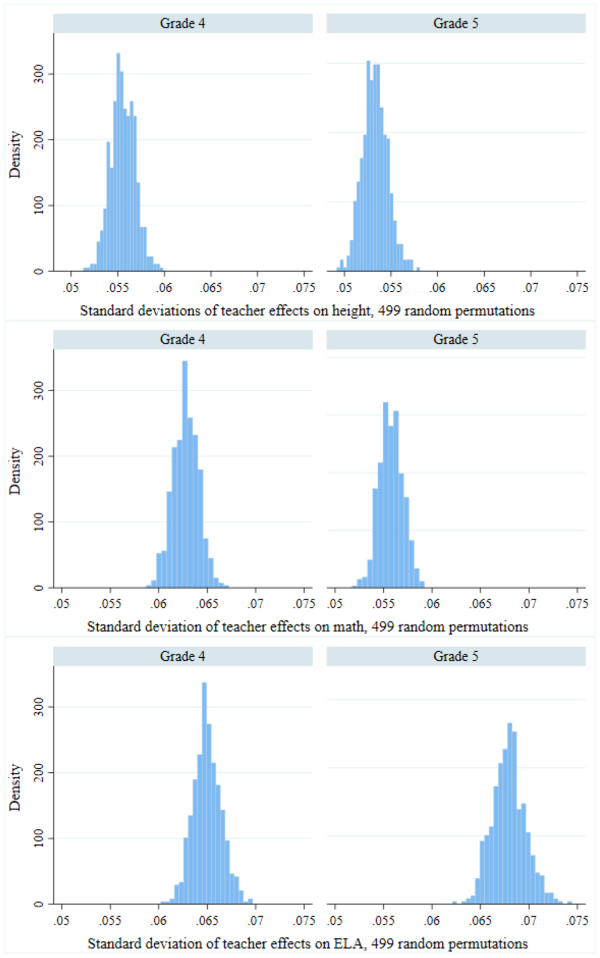
Standard deviation of teacher effects from 499 random permutations of students to teachers

Notes: To create these figures, we repeated the following steps 499 times. First, randomly allocate all students in our data to teachers (within year, maintaining the same number of students per teacher). Then, re-estimate the value-added model assuming fixed effects. (Standard deviations of the adjusted fixed effects are shown). For each iteration, we saved the estimated standard deviation in teacher effects. These figures show the distribution of these across random permutations, where the null that there are no true teacher effects has been imposed.

In the fixed effects models, the average $\widehat{{\sigma }_u}$ across permutations ranged from 0.053 for height to 0.068 for ELA. The standard deviation of these estimates across permutations is roughly 0.001–0.002. In other words, even when (real) data on students is randomly allocated across teachers, a 1σ increase in teacher “value-added” is associated with an average 0.053σ increase in height and a 0.068σ increase in ELA test performance. Figure 3 shows also that the vast bulk of the distribution of these “null” standard deviations is well below our estimates of the standard deviation of teacher effects for height and achievement from the actual data, suggesting the standard deviations from the actual data are statistically significantly different from 0. As one would expect, teacher effects under random assignment of students to teachers are uncorrelated with those estimated with the actual data. (They are also uncorrelated across subjects.)¹⁵

The permutation test offers two important insights. First, even under completely random assignment of student data to teachers, there are significant teacher “effects” in our 2-level models. The distribution of effects under random permutations provides a sense of the range of standard deviations under an imposed null of no systematic sorting, peer effects, or true effects. Second, our estimated teacher effects in the observed data are clearly over-dispersed relative to this null effect distribution, suggesting our estimated teacher effects on height and achievement have a standard deviation that is statistically different from zero. To take one example, the 95^th percentile of the ${\widehat{\sigma }}_u$ for 4^th grade height among permutations is 0.06 (Figure 3). This can be compared to an estimated ${\widehat{\sigma }}_u$ in the actual data of 0.218. Similar differences are observed in math and ELA. In the case of height, this suggests that there is some systematic variation beyond randomness associated with the actual class sizes within schools and sampling variation in the covariates.

Next, we investigate the role of idiosyncratic error by estimating the more sophisticated 3-level models that include a random classroom error that is uncorrelated within teachers over time. While this approach is less common in the literature and in practical settings than the traditional 2-level model, it is the one used by Kane, Staiger, and Rockoff (2008) and Chetty et al. (2014a). As discussed above, we estimate this 3-level model using maximum likelihood; the Kane, Staiger, and Rockoff (2008) approach; and the Chetty et al. (2014a) drift model. The key difference between the first and the latter two approaches is that the “signal” component of the shrinkage factor is estimated from the covariance in classroom effect for the same teacher in successive years. Our results in the previous section suggested this covariance is close to zero for these estimates of teacher effects on height. The shrinkage factor using this method would be the theoretically “correct” one if there were no persistent teacher effects on height.

Panel B of Table 4 reports the estimated standard deviations in teacher effects on achievement and height when fitting 3-level models. The estimates in panel (B) come from the mean residuals (KRS) approach or maximum likelihood estimation (MLE), as indicated. For each of these models, the standard deviation in teacher effects on height falls to zero, while those for math and ELA remain significant, ranging from 0.087–0.199, depending on the model, grade, and subject.¹⁶ The Chetty et al. model of teacher effects with “drift” yields a non-zero standard deviation of teacher effects for height (0.057 for 4^th grade and 0.031 for 5^th grade), but these values are no larger than those obtained in the permutation test. Thus, it is no larger than what one might find by chance. These results suggest that the estimated effects in our baseline models for height are almost certainly not “true” effects on height, but rather idiosyncratic classroom-level error.

6. Discussion

As of the 2015–16 school year, 36 of 46 states implementing new teacher evaluation systems had incorporated some version of VAMs or comparable student achievement growth measures into their annual teacher evaluations (Steinberg & Donaldson 2016). Value-added models are appealing to school district leaders and state education agencies in part because of their convenience. Unlike observational protocols—which require trained raters to periodically visit every classroom at considerable expense—VAMs use existing administrative data and can be calculated centrally. The case for VAMs is also supported by a growing body of research documenting a relationship between measures of teacher value-added and students’ long-run outcomes (e.g., Chetty et al. 2014b).

Nonetheless, VAMs remain controversial as a human resources tool in part because of concerns about bias and idiosyncratic error (American Statistical Association 2014). These concerns each raise the possibility that VAMs may improperly attribute differences in student outcomes to teachers. With respect to bias, the error is systematic: the model is mis-specified or does not account for other causal influences on student outcomes related to teacher assignment but outside of the teacher’s influence. Idiosyncratic error is random by definition: on average a VAM may be “correct,” but any given estimate may depart significantly from the teacher’s true impact, especially for newer teachers.

The question of whether VAMs are unbiased and imprecise has been given considerable attention in the literature. This paper departs from previous work by fitting commonly estimated value-added models to an outcome that teachers cannot plausibly effect: student height. Our analysis uses real data, available for the same set of NYC students whose achievement data were used to produce value-added estimates for teachers. Height is arguably measured with less error than student achievement. However, height—like achievement—can vary in idiosyncratic ways across classrooms. This variation may be due to measurement error, shocks unrelated to teachers, or sampling variation. We find large and statistically significant effects of teachers on height using a wide range of 2-level value-added model specifications commonly used in practice. In our case, the only specifications that resulted in the theoretically expected effects of zero were models that “shrank” estimated teacher effects by separating “persistent” teacher effects from idiosyncratic classroom-level error (e.g., Kane, Rockoff, and Staiger 2008; Chetty et al. 2014a). We found little evidence of student sorting to teachers on factors related to height (or changes in height) that might suggest bias in teacher value-added measures on achievement from this sorting.

These findings are reassuring in the sense that they support statistical models that successfully separate persistent effects from random or classroom-level error, at least for our measure where the null of zero effects is clear. That said, this 3-level model is rarely used in on-the-ground teacher evaluation systems. This is in part because practitioners are interested in current, time-varying measures of teacher performance that are responsive to changes in teacher practice and effort. True teacher effectiveness may also vary in response to real shocks to performance, such as illness or professional development. The 3-level model is not designed to capture short-term fluctuation in teacher effects relevant for teacher performance evaluation. Moreover, high-stakes applications of VAMs concern more than just the question of whether “effects” are globally zero or not; individual estimates—which contain both signal and noise—must be sufficiently reliable to make personnel decisions. The 3-level models we estimated would (rightfully) suggest that use of such VAM models to estimate teacher effects on height do not lead to spurious non-zero estimates. We thus interpret our results as a cautionary tale for the naïve application of VAMs with 2-level models in educational and other settings. Future work could use simulated data to further explore the role of noise in generating false “effects” or affecting individual estimates.

References

- Aaronson Daniel, Barrow Lisa, and Sander William. 2007. “Teachers and Student Achievement in the Chicago Public High Schools,” Journal of Labor Economics 25: 95–135. [Google Scholar]
- American Institutes for Research. 2013. 2012–2013 Growth Model for Educator Evaluation: Technical Report Prepared for the New York State Education Department. Washington, D.C.: American Institutes for Research. [Google Scholar]
- Bacher-Hicks A, Chin MJ, Kane TJ, & Staiger DO 2017. “An Evaluation of Bias in Three Measures of Teacher Quality: Value-Added, Classroom Observations, and Student Surveys.” National Bureau of Economic Research Working Paper Series, No. 23478. [Google Scholar]
- Bacher-Hicks A, Kane TJ, & Staiger DO 2014. “Validating Teacher Effect Estimates Using Changes in Teacher Assignments in Los Angeles.” National Bureau of Economic Research Working Paper Series, No. 20657. [Google Scholar]
- Baker EL, Barton PE, Darling-Hammond L, Haertel E, Ladd HF, Linn RL, et al. 2010. Problems with the Use of Student Test Scores to Evaluate Teachers. Economic Policy Institute Briefing Paper No. 278. [Google Scholar]
- Ballou D, Mokher CG, and Cavalluzzo L 2012. “Using Value-Added Assessment for Personnel Decisions: How Omitted Variables and Model Specification Influence Teachers’ Outcomes.” Working paper. [Google Scholar]
- Ballou D, Sanders W, and Wright P 2004. “Controlling for Student Background in Value-Added Assessment of Teachers.” Journal of Educational and Behavioral Statistics, 29: 37–65. [Google Scholar]
- Braun HI, Chudowsky N, & Koenig J 2010. Getting Value Out of Value-Added: Report of a Workshop. Washington, D.C.: National Academies Press. [Google Scholar]
- Briggs DC and Domingue B (2013). “The Gains from Vertical Scaling.” Journal of Educational and Behavioral Statistics 38(6): 551−−576. [Google Scholar]
- Buddin Richard, and Zamarro Gema. 2009. “Teacher Qualifications and Student Achievement in Urban Elementary Schools,” Journal of Urban Economics 66: 103–115. [Google Scholar]
- Chetty R, Friedman JN, & Rockoff JE 2014a. “Measuring the Impacts of Teachers I: Evaluating Bias in Teacher Value-Added Estimates.” American Economic Review, 104(9), 2593–2632. [Google Scholar]
- Chetty R, Friedman JN, & Rockoff JE 2014b. “Measuring the Impacts of Teachers II: Teacher Value-Added and Student Outcomes in Adulthood.” American Economic Review, 104(9), 2633–2679. [Google Scholar]
- Chetty R, Friedman JN, & Rockoff JE 2017. “Measuring the Impacts of Teachers: Reply.” American Economic Review, 107(6), 1685–1717. [Google Scholar]
- Doherty Kathryn M., and Jacobs Sandi. 2013. Connect the Dots: Using Evaluations of Teacher Effectiveness to Inform Policy and Practice. Washington, D.C.: National Council on Teacher Quality. [Google Scholar]
- Glazerman S, Loeb S, Goldhaber D, Staiger D, Raudenbush S, and Whitehurst G 2010. “Evaluating Teachers: The Important Role of Value-Added.” Washington, D.C.: Brookings Institution. [Google Scholar]
- Glazerman S, Goldhaber D, Loeb S, Raudenbush S, Staiger DO, and Whitehurst GJ 2011. “Passing Muster: Evaluating Teacher Evaluation Systems.” Washington, D.C.: Brookings Institution. [Google Scholar]
- Goldhaber D, & Chaplin D 2011. “Assessing the ‘Rothstein Test’: Does it Really Show Teacher Value-Added Models are Biased?” Washington, D.C.: CALDER Center Working Paper; No. 71. [Google Scholar]
- Goldhaber D, and Hansen ML 2012. “Is It Just a Bad Class? Assessing the Long-Term Stability of Estimated Teacher Performance,” Economica 80: 589–612. [Google Scholar]
- Goldhaber DD, Goldschmidt P, and Tseng F 2013. “Teacher Value-Added at the High-School Level: Different Models, Different Answers?” Educational Evaluation and Policy Analysis, 35: 220–236. [Google Scholar]
- Gordon Robert, Kane Thomas J., and Staiger Douglas O.. 2006. “Identifying Effective Teachers Using Performance on the Job.” Washington, D.C.: Brookings Institution. [Google Scholar]
- Guarino CM, Maxfield M, Reckase MD, Thompson P, and Wooldridge JM 2015. “An Evaluation of Empirical Bayes’ Estimation of Value-Added Teacher Performance Measures.” Journal of Educational and Behavioral Statistics, 40(2), 190–222. [Google Scholar]
- Hanushek Eric A. 2009. “Teacher Deselection,” in Creating a New Teaching Profession, Goldhaber Dan and Hannaway Jane (eds.) Washington, D.C.: The Urban Institute Press. [Google Scholar]
- Hanushek EA, and Rivkin SG 2010. “Generalizations about Using Value-Added Measures of Teacher Quality.” American Economic Review, 100: 267–271. [Google Scholar]
- Harris Douglas, and Sass Tim R.. 2006. “Value-Added Models and the Measurement of Teacher Quality,” Working Paper, Florida State University. [Google Scholar]
- Harris Douglas N. 2011. Value-Added Measures in Education What Every Educator Needs to Know. Cambridge: Harvard Education Press. [Google Scholar]
- Harris DN, Ingle WK, & Rutledge SA 2014. “How Teacher Evaluation Methods Matter for Accountability: A Comparative Analysis of Teacher Effectiveness Ratings by Principals and Teacher Value-Added Measures.” American Educational Research Journal, 51: 73–112. [Google Scholar]
- Hill HC, Kapitula L,& Umland K 2011. A Validity Argument Approach to Evaluating Teacher Value-Added Scores. American Educational Research Journal, 48: 794–831. [Google Scholar]
- Horvath Hedvig. 2015. “Classroom Assignment Policies and Implications for Teacher Value-Added Estimation.” Job Market Paper, University of California-Berkeley Department of Economics. [Google Scholar]
- Isenberg E, and Hock H 2011. Design of Value-Added Models for IMPACT and TEAM in DC Public Schools, 2010–2011 School Year: Final Report. Washington, DC: American Institutes for Research. [Google Scholar]
- Ishii J, and Rivkin SG 2009. “Impediments to the Estimation of Teacher Value Added.” Education Finance and Policy, 4: 520–536. [Google Scholar]
- Jackson CK, Rockoff JE, & Staiger DO 2013. “Teacher Effects and Teacher-Related Policies.” Annual Review of Economics. [Google Scholar]
- Kane MT 2017. “Measurement Error and Bias in Value-Added Models.” ETS Research Report Series 2017(1): 1–12. [Google Scholar]
- Kane TJ, McCaffrey DF, Miller T, and Staiger DO 2013. “Have We Identified Effective Teachers? Validating Measures of Effective Teaching Using Random Assignment.” Seattle, WA: Gates Foundation. [Google Scholar]
- Kane Thomas J., Rockoff Jonah E., and Staiger Douglas O.. 2008. “What Does Certification Tell Us About Teacher Effectiveness? Evidence from New York City,” Economics of Education Review 27: 615–631. [Google Scholar]
- Kane Thomas J., and Staiger Douglas O.. 2008. “Estimating Teacher Impacts on Student Achievement: An Experimental Evaluation,” National Bureau of Economic Research Working Paper #14607. [Google Scholar]
- Kinsler J 2012. “Assessing Rothstein’s Critique of Teacher Value-Added Models. Quantitative Economics, 3(2), 333–362. [Google Scholar]
- Koedel C, and Betts JR 2011. “Does Student Sorting Invalidate Value-Added Models of Teacher Effectiveness? An Extended Analysis of the Rothstein Critique.” Education Finance and Policy, 6: 18–42. [Google Scholar]
- Koedel C, Mihaly K and Rockoff JE (2015). “Value-added modeling: A review.” Economics of Education Review 47: 180−−195. [Google Scholar]
- Mead S (2012). Recent state action on teacher effectiveness. Washington, DC. Bellwether Education Partners. Retrieved from http://bellwethereducation.org/sites/default/files/RSA-Teacher-Effectiveness.pdf [Google Scholar]
- McCaffrey Daniel F., Sass Tim R., Lockwood JR, and Mihaly Kata. 2009. “The Intertemporal Variability of Teacher Effect Estimates,” Education Finance and Policy 4: 572–606. [Google Scholar]
- Rockoff Jonah E. 2004. “The Impact of Individual Teachers on Student Achievement: Evidence from Panel Data.” American Economic Review, Papers and Proceedings of the American Economic Association. 94: 247–252. [Google Scholar]
- Rockoff JE, Staiger DO, Kane TJ, and Taylor ES 2012. “Information and Employee Evaluation: Evidence from a Randomized Intervention in Public Schools.” American Economic Review, 102(7), 3184–3213. [Google Scholar]
- Rothstein Jesse. 2010. “Teacher Quality in Educational Production: Tracking, Decay, and Student Achievement.” Quarterly Journal of Economics 125: 175–214. [Google Scholar]
- Rothstein Jesse. 2017. “Measuring the Impacts of Teachers: Comment.” American Economic Review, 107(6), 1656–1684. [Google Scholar]
- Schochet Peter Z. and Chiang Hanley S.. 2013. “What Are Error Rates for Classifying Teacher and School Performance Using Value-Added Models?” Journal of Educational and Behavioral Statistics, 38: 142–171. [Google Scholar]
- Soland J (2017). “Is Teacher Value Added a Matter of Scale? The Practical Consequences of Treating an Ordinal Scale as Interval for Estimation of Teacher Effects.” Applied Measurement in Education 30(1): 52–70. [Google Scholar]
- Weisburg Daniel, Sexton Susan, Mulhern Susan, and Keeling David. 2009. The Widget Effect: Our National Failure to Acknowledge and Act on Differences in Teacher Effectiveness. The New Teacher Project. [Google Scholar]
Associated Data
This section collects any data citations, data availability statements, or supplementary materials included in this article.