

Abstract
Semantic segmentation is an important step in understanding the scene for many practical applications such as autonomous driving. Although Deep Convolutional Neural Networks-based methods have significantly improved segmentation accuracy, small/thin objects remain challenging to segment due to convolutional and pooling operations that result in information loss, especially for small objects. This paper presents a novel attention-based method called Across Feature Map Attention (AFMA) to address this challenge. It quantifies the inner-relationship between small and large objects belonging to the same category by utilizing the different feature levels of the original image. The AFMA could compensate for the loss of high-level feature information of small objects and improve the small/thin object segmentation. Our method can be used as an efficient plug-in for a wide range of existing architectures and produces much more interpretable feature representation than former studies. Extensive experiments on eight widely used segmentation methods and other existing small-object segmentation models on CamVid and Cityscapes demonstrate that our method substantially and consistently improves the segmentation of small/thin objects.
Index Terms—: Small-object Semantic Segmentation, Across Feature Map Attention
1. Introduction
Semantic segmentation is an important processing step in natural or medical image analysis for the detection of distinct types of objects in images [1]. In this process, a semantic label is assigned to each pixel of a given image. The breakthrough of semantic segmentation methods came when fully convolutional neural networks (FCN) were first used by [2] to perform end-to-end segmentation of images. While semantic segmentation has achieved significant improvement based on the conception of fully convolutional networks, small and thin items in the scene remain difficult to segment because the information of small objects is lost throughout the convolutional and pooling processes [3], [4], [5], [6]. For example, Fig. 1a is an image of size 800 by 1200 pixels, which contains two cars: the larger car is 160 by 220 pixels (Fig. 1b), and the smaller one is 30 by 40 (Fig. 1c). After a convolution operation with a convolution kernel of 10×10, the length and width of the image are compressed to one-tenth of the original size (as shown in Fig. 1d). Accordingly, the dimensions of the large and small cars become 16 by 22 and 3 by 4 pixels, respectively. As seen from the example, we can still see the car’s features from Fig. 1e (feature map of the large car), but we can hardly see the features of the small car from the 12-pixel size Fig. 1c (feature map of the small car). This is because the high-level representation from convolutional and pooling operations generated along lowers the resolution, which often leads to the loss of the detailed information of small/thin objects [3] — as a result, recovering the car information from the coarse feature maps is difficult for segmentation models [7]. However, accurately segmenting small objects is critical in many applications, such as autonomous driving, where the segmentation and recognition of small-sized cars and pedestrians in the distance is critical [8], [9], [10], [11].
Fig. 1.

Example of the convolution operation. The example employs convolution with a kernel of size 10 by 10 with parameters all set one, where stride is 10. The output of this convolution operation is one-hundredth of the original input pixels. (a) The original image of size 800×1200 pixels. (b) The larger car in the original image has a resolution of 160×220 pixels. (c) represents the smaller car which has a resolution of 30×40 pixels. (d) The original image’s feature map that generated by the convolution operation. It is one-tenth the length and width of the original image, respectively. (e) The feature map of the large car. (f) The feature map of the small car. (g) The relationship between the small car (c) and the feature map (d). (h) Improving the performance by utilizing the obtained relations and the large car’s output.
Some methods for small object segmentation have been proposed [6], [9], [10], [12], [13], [14], [15], [16], [17], [18], [19], [20], [21], [22], [23], [24], [25]. A common strategy is to scale up the input images to improve the resolution of small objects or generate high-resolution feature maps [6], [9], [10], [12], [13]. The strategy relying on data augmentation or feature dimension increment generally results in significant time consumption for training and testing. Another promising strategy is to develop network variants, such as skip connections [14], hypercolumns [15], [16], feature pyramids [17], [18], [19], dilated convolution [20], [21], to enhance high-level small-scale features with multiple lower-level features layers. The strategy of integrating multi-scale representation cannot ensure the feature alignment of the same object and the features are not interpretable enough for semantic segmentation [10], [25]. Post-processing, such as Markov Random Field and Conditional Random Field-based post-processing [22], [23], is another strategy to improve the small object segmentation. Since post-processing is a separate part of the training of the segmentation model, the network cannot adapt its weights based on the post-processing outputs [24], [25].
In this paper, we present a novel small-object sensitive segmentation strategy without relying on increasing the data scale, enlarging the image/feature sizes, or modifying the network architecture. Noticing that the same object category often shares similar imaging characteristics, we propose to leverage the relation among the small and large objects within the same category to compensate for the information loss from the feature propagation. For example, Fig. 1b and Fig. 1c show that the large and small cars are very similar despite their vastly different sizes, the output of the large car can be used to correct the results of the small car region if we know the different image regions represent the same type of object. However, directly calculating the degree of similarity from the input image can be quite challenging since the size of different objects can be vastly different. We hereby propose to quantify this relation by delving deeper into the feature space. This is motivated by the fact that the size of the small object in imaging space and the large object in feature space have more comparable size. For example, Fig. 1c and Fig. 1e show that the small car in the original image and the large car in the feature map have similar sizes and characteristics. We can derive the relation between the small and large cars by exploiting the original image of small car and the feature map of large car. To this end, we present Across Feature Map Attention (AFMA), which represents the similarities of objects in the same category by calculating the cross-correlation matrices between the intermediate feature patches and the image patches. The relation can then be utilized to enhance small object segmentation. For example, combining the relation of the small and large cars (Fig. 1g) and the output of the large car can compensate for the information loss of the small car (Fig. 1h). To further improve the quality of the obtained relation (i.e., AFMA), we propose to use the gold AFMA, which is computed based on the groundtruth segmentation mask, to constitute extra supervision.
As shown in Fig. 2, our method is an efficient plug-in which can be easily applied to a wide range of popular segmentation networks. To demonstrate its effectiveness, we comprehensively evaluate our method on eight segmentation models and two urban street scene datasets. The experimental results show that our method consistently improves the segmentation accuracy, especially for the small object classes. To conclude, the main contributions of this paper are:
We propose a novel method, i.e., Across Feature Map Attention, to fully exploits the relation of objects in the same category, for enhancing small object segmentation.
To the best of our knowledge, we present the first method to characterize attention by finding the relationship between different levels of feature maps.
Unlike previous methods which applies data augmentation or multi-scale processing, our AFMA provides much more interpretable features (see Sec. 4.4 and Sec. 4.5).
The proposed AFMA is lightweight and can be easily plugged into a wide range of architectures. For instance, DeepLabV3, Unet, Unet++, MaNet, FPN,PAN, LinkNet, and PSPNet achieve 2.5%, 4.7%, 3.0%, 3.0%, 2.5%, 5.0%, 4.0%, and 2.9% improvement with only less than 0.1% parameters increment.
Fig. 2.

The overview of our method. (a) represents an overview of combining the AFMA method with a general semantic segmentation method. The encoder of the segmentation model is input to the AFMA method, and its output is applied to the output of the segmentation method. (b) presents a detailed illustration of combining the AFMA method with different semantic segmentation models. It can be observed that the AFMA approach is adaptable to different types of architectures of various semantic segmentation models and can work on different layers of the encoder’s feature maps.
We release our codes as well as data processing procedures for the public datasets, so that other researchers can easily reproduce our results1.
2. Related Work
2.1. Semantic Segmentation
Most semantic segmentation approaches introduced in recent years have focused on increasing segmentation accuracy based on the FCN architecture [2], which focuses on drawing information from the input image and then using these derived features to construct the final segmentation image. Encoder-decoder is the widely adopted structure to improve FCN by considering spatial details and contexts. SegNet [26], a fully convolutional encoder-decoder architecture-based method, upsamples its lower-resolution input feature map(s) by using pooling indices computed in the max-pooling step. Furthermore, LinkNet [27], W-Net [28], HRNet [29], Stacked Deconvolutional Network [30], etc., adopt transposed convolutions or feature reuse strategies to overcome the shortcoming of fine-grained image information loss based on encoder-decoder architecture. Based on the encoder-decoder structure, Unet [14] integrates the feature maps of the encoder and decoder by dense skip connections to fully leverage the features from each layer. The features from each layer in the encoder part are connected to the symmetrical layers in the decoder part. Many extensions of UNet, such as Unet++ [31],mUnet [32], 3D-Unet [33] and stacked UNets [34], have been proposed for various problem areas. Subsequently, pyramid pooling and dilated convolution (also called atrous convolution) have been widely used to enhance the resolution of feature maps and enlarge the receptive field. Pyramid Scene Parsing Network (PSPNet) [18] adopts a multi-scale network for better learning the global context representation of a scene. DeepLab [21], DeepLabV3 [17], multiscale context aggregation [20], densely connected Atrous Spatial Pyramid Pooling [35], and Efficient Network [36] use large rate dilated/atrous convolutions to enlarge the receptive field and capture broader scope context information. Attention mechanisms have also been explored in semantic segmentation to assess the importance of features at different positions and scales [37]. Pyramid Attention Network (PAN) [38] combines attention mechanisms and spatial pyramids to extract specific dense features for semantic segmentation. Multi-scale Attention Net (MANet) [39] exploits self-attention to integrate local features with their global dependencies adaptively. Gated Fully Fusion [3] uses a gating mechanism (similar to attention mechanism) to fuse features from different feature maps selectively. The gating mechanism measures the usefulness of features and control information propagation through gates accordingly. In this paper, we select eight representative and widely used semantic segmentation models related to encoder-decoder, skip connection, pyramid pooling and dilated convolution, or attention mechanism as baseline models in our experiments.
2.2. Small Object Segmentation
The information of small and thin items will be lost as the network deepens due to the convolutional and pooling processes. Some specific methods for small object segmentation have been proposed [6], [9], [10], [12], [13], [14], [15], [16], [17], [18], [19], [20], [21], [22], [23], [24], [25]. One common strategy is to scale up the input images to improve the resolution of small objects or generate high-resolution feature maps [6], [9], [10], [12], [13]. The strategy relying on data augmentation or feature dimension increment generally results in significant time consumption for training and testing. Another promising strategy is to develop network variants, such as skip connections [14], hypercolumns [15], [16], feature pyramids [17], [18], [19], dilated convolution [20], [21], to use multi-scale feature layers, which has the effect of zooming in small objects. Although the feature pyramid structure and dilated convolutions help overcome this issue, the small objects still cover too little practical information to be effectively recognized [4]. Post-processing, such as Markov Random Field and Conditional Random Field-based post-processing [22], [23], is another strategy to improve the small object segmentation. Since post-processing is a separate part of the training of the segmentation model and the network cannot adapt its weights based on the post-processing outputs [24], [25]. Changing the loss function is another way to improve small object segmentation. In [26], the loss function adopts the median frequency balancing weights for training, and it proposes to assign different training weights to objects of various sizes. Guo et al. [25] presented a small object boundary-sensitive loss function to improve small object recognition. The advantage of changing the loss function is that it does not introduce extra computational cost to the segmentation model. However, the improvement of small object segmentation is not interpretable enough for semantic segmentation. Here, we present a new method that could improve the small object segmentation with a very small extra computation cost and is also more convenient for interpretation.
2.3. Attention Networks
The attention mechanism is widely used in semantic segmentation to select significant features. Several methods adopt global attention to utilize the global scene context for segmentation. Pyramid Attention Network [38] presents a global attention upsampling method to extract specific dense features for semantic segmentation. Global Recurrent Localization Network [40] obtains attention maps from encoded features to attend to the global contexts. PiCANets [41] presents global and local attention modules for capturing global and local settings in low- and high-resolution, respectively. Chen et al. [42] used hierarchical structures of attention maps to attend to global contexts at all scales. Pixel attention is used to capture the relationship between two pixels. The Multi-scale Attention Net [39] uses pixel attention to integrate local elements with their global dependencies. Wang et al. [42] designed a non-local operation that computes interactions between two locations to capture long-range relationships directly. Squeeze-and-excitation first uses global average pooling and then passes through multilayer perceptrons to obtain Channel attention to improve models’ performance. DFN [43] uses global average pooling to bring channel-wise attention into the network while selecting the selection of more discriminative features. Attention Complementary Network (ACNet) [44] is a channel attention-based module that extracts weighted features from initial image and depth branches. Zhang et al. [45] progressively utilized both spatial and channel-wise attention to integrate multiple contextual information of multi-level features. In this paper, we propose across feature maps attention to find the relation between small and large objects, for enhancing small object segmentation.
3. Method
3.1. Overview
As shown in figure Fig. 2a, the pipeline consists of a default segmentation network and our proposed method. The default segmentation network can be any segmentation model, and our approach takes the model’s encoder as input, and its output is added to the output of the decoder.
Specifically, the general semantic segmentation architecture consists of an encoder and a decoder. The encoding part is used for feature representation learning, while the decoder is for pixel-level classification. Our method first computes the Across Feature Map Attention (AFMA), which aims to quantify the relation between each input image and the corresponding feature maps, i.e., the output from the intermediate encoding layers (see Section 3.2). Then the derived AFMA is used to modulate the output from the decoder (see Section 3.3). In addition, we propose to compute the gold AFMA (see Section 3.4) based on the groundtruth segmentation mask for better guiding the learning of AFMA. During the training, the overall objective is comprised of both the standard segmentation loss and an additional AFMA loss in order to let the learned AFMA approach the gold AFMA (see Section 3.5). The overall framework of our method is illustrated in Fig. 3.
Fig. 3.

The framework of our method. (a) Calculate the Across Feature Map Attention. The inputs are the initial image and i-th layer feature maps of the encoder. (b) Output Modification. The generated AFMA in (a) is used to modify the output of the decoder’s predicted masks. (c) The process of generating gold AFMA.
3.2. Across Feature Map Attention (AFMA)
The proposed AFMA aims to model the relationship between small and large objects. Specifically, AFMA computes the cross-correlation between the patches of original image and the patches of corresponding feature maps. By compensating for the information loss from the feature propagation, AFMA effectively boosts the segmentation performance, especially from those small objects. Given a color image as input, the encoder of the segmentation model extracts the feature maps , where and denote width, height, and the number of channels of the feature maps, respectively. Our model takes the first level feature map of encoder (the original input image) and i-th layer feature map as input to generate the AFMA, we introduce the detailed process as following the serial numbers shown in Fig. 3a.
Step ①. One convolutional layer with 64 filters and one convolutional layer with 1 filter are used to embed the first level feature maps (the image I). In particular, we formulate this procedure as Eq. (1):
| (1) |
where .
Step ②. Given the i-th level feature maps , one convolutional layer with filters convert the i-th level feature maps to per category features. Eq. (2) describes the procedure
| (2) |
where , is the number of categories to predict. We hypothesize only contains the information associated with the k-th category.
Step ③. In this step, we split into fixed-size patches. The procedure is described as Eq. (3)
| (3) |
The procedure follows [46], is the image partition operation which reshapes the into a sequence of flattened 2D patches . The j-th vector of contains a resolution patch of the image2.
Step ④. Similar to step ③, we partition each channel of into a sequence of flattened patches, respectively.
| (4) |
| (5) |
where is the sequence of flattened 2D patches of represents concatenation and .
Step ⑤. The dot product is adopted between and each of to determine the relationship between each image patch of the original image and the k-th categoryrelated feature map. Eq. (6) and Eq. (7) describe the procedure.
| (6) |
| (7) |
where is the transposed matrix of , and represents the associations between each image patch of the original image and each image patch of the k-th category-related feature map.
3.3. Probability/Output Modulation
The obtained attention map is then applied to modulate the output of the decoder, so as to enhance the segmentation from those small objects (Fig. 3b). The general segmentation network outputs a predicted masks for the input image , where
| (8) |
The predicted masks are softly exclusive to each other, i.e., , and each pixel’s predicted mask denotes the probability of assigning class k to the j-th pixel.
Step ⑥. We use fixed-sized average pooling to compress the output of decoder to the same size as . The procedure is described as Eq. (9) and Eq. (10)
| (9) |
| (10) |
where and . (input, ) denote average pooling with kernel size and stride . For each pixel from is:
| (11) |
We can know from Eq. (11) that similarly to , the compressed masks are softly exclusive to each other, i.e., . The value of each pixel represents the probability of assigning class k to the compressed pixel.
Step ⑦. Same as steps ③ and ④, we partition each channel of into a sequence of flattened patches.
| (12) |
| (13) |
where and .
Step ⑧. In this step, the attention map is applied on top of to spatially modulate the output probability.
| (14) |
| (15) |
where and . Since contains the predicted masks for compressed image patch, and represents the relation between the initial image patches (containing relative small objects) and the feature patches (containing relative large objects). represents the influence of the output of large objects on small objects.
Step ⑨. We fold the to the same size of :
| (16) |
| (17) |
where and . denotes the operation of folding the input by . represents the modification generated from the i-th feature maps, and the final prediction Pre of our method is:
| (18) |
where
3.4. Gold AFMA Computation
We define the gold AFMA , which is computed based on the groundtruth segmentation mask. During the training process, the gold AFMA will be used to provide supervision for A, for further improving the quality of the attention map.
Step ⑩. Fig. 3c illustrates the process of calculating the gold AFMA. For the groundtruth labels , the groundtruth masks do not overlap with each other, i.e.,
| (19) |
| (20) |
| (21) |
where . Each value of represents the gold relationship between original image’s patch and feature maps’ patch.
Fig. 4 is an illustration of the gold AFMA calculation. Assume we have an initial input image of which contains two types of objects: square and cross. The groundtruth labels are two matrices denoted as and , respectively. According to Eq. (19), we use average pooling operation to compress the groundtruth into and , respectively. Then following Eq. (20), image partition operation and are first acted on the compressed groundtruth, which obtain two flatten patched image matrices and . Similarly, we perform image partition operations and to the original image, and the partition image patches and are obtained. Following Eq. (20), the and are generated by matrix multiplication operation. Fig. 4 shows four examples of calculating the values of and :
Fig. 4.
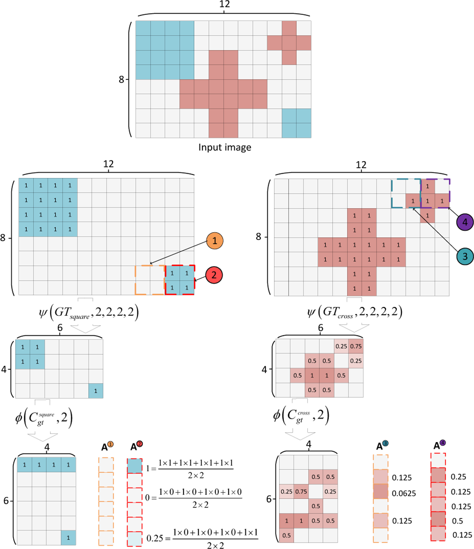
An illustration of calculating gold AFMA. The 0 in the gold standard masks is not presented.
Square related AFMA:
As shown in Fig. 4, there is no square-related pixel (the pixels that make up squares) in image patch  (yellow dashed line). Thus we can observe that the
  are all zeros, which means there is no relationship between image patch and all other image patches of . For image patch
  (red dashed line), all pixels in this image patch belong to square. As a result, we can see from Fig. 4 that the
  is strongly related to the image patch of the compressed large square (the value is 1) and also has a relatively strong relationship with the image patch of the compressed smaller square (the value is 0.25).
Cross related AFMA:
The Fig. 4 shows that there are 1 and 3 cross-related pixels in image patch  (blue dashed line) and
  (purple dashed line), respectively. As a result, image patch has stronger relations with each compressed large cross than image patch (
 value is greater than
  at each position). From the above examples, we know that the more the image patch of the original image contains pixels of a specific object, the more it is related to the image patch of feature maps of that object.
The  ,
,  , , and
  are used on the output of the general segmentation model’s decoder (as shown in Sec. 3.3). Since the values of are zeros, the predicted masks of the large square have no impact on the results of image patch but have a significant effect on the results of image patch due to has a strong relationship with the image patch of the compressed large square. Similarly, the prediction of the large cross will have more influence on the output of image patch than since image patch of the original image contains more small cross-related pixels.
3.5. Training Losses
The overall training objective consists of two loss terms: 1 ) the standard segmentation loss, which aims to minimize the difference between the prediction and the groundtruth segmentation mask; 2) the AFMA loss, which aims to minimize the difference between the learned AFMA and the gold AFMA. For the segmentation loss, we follow [26] and adopt the median frequency balancing weighted sigmoid cross-entropy loss for training:
| (22) |
where denotes the groundtruth (0 or 1) of class k at pixel , and denotes the the k-th probability of the final prediction at . denotes the median frequency weight assigned to category k. For the AFMA, we use mean square error (MSE) loss for training:
| (23) |
where (as shown in Eq. (7)) and (as shown in Eq. (21)) are the predicted and the gold AFMA, respectively. Then the overall training objective consists of the two losses:
| (24) |
4. Experiments
4.1. Datasets and Evaluation Measures
We evaluate our proposed method on two well known urban street datasets: CamVid [47] and Cityscape [48]. The CamVid dataset is a road scene segmentation dataset of practical interest for various autonomous driving-related problems. The dataset consists of 367 training images, 100 validation images, and 233 testing images. In total, 11 semantic classes are annotated by pixel-level. The resolution of the images is . We define sign symbol, pedestrian, pole, and bicyclist as small-object classes based on the item size [10] as other’s defined in [25]. The remaining seven object classes are all denoted as large-object classes. The Cityscapes dataset is a recently released dataset for semantic urban street scene understanding. The dataset includes 5,000 precisely annotated pixel-level images: 2,975 training images, 500 validation images, and 1,525 testing images. The resolution of the image is . In addition, Cityscapes provides 20,000 coarsely annotated images. In this paper, we consider only the fine annotations for training. There are a total of 19 semantic classifications in Cityscapes. We define pole, traffic light, traffic sign, person, rider, motorcycle, and bicycle as small-object classes based on the object size [10]. All the other 12 object classes are designated as large-object classes. CamVid dataset provides the ground-truth segmentation labels for the training, validation, and testing. Cityscapes only provides the ground-truth labels for the training and validation datasets, the ground-truth for the testing dataset is withheld from the user. The testing results of the Cityscapes dataset are obtained via online submissions.
The metrics used for segmentation performance evaluation in this paper are: Class intersection over union (IoU), mean intersection over union (mIoU), mean small-object class intersection over union , and mean large-object class intersection over union .
4.2. Implementation Details
We directly trained all models from scratch on CamVid and Cityscapes without pre-training the backbone on the ImageNet [49]. We have not used any coarse labeled images or any extra data in this work. In all experiments, we conduct our models by PyTorch3, and all baseline segmentation models used in the experiments are implemented using SMP4.
We use mini-batch stochastic gradient descent (SGD) with momentum 0.9, weight decay of 5e4 and adaptive learning rates. The batch size is set to 16, 8 for the CamVid and Cityscapes dataset, respectively. Data augmentation contains random horizontal flip with probability 0.5, random crop, and random resize with scale range [0.5, 2.0]. The cropped resolution is 480× 640 for training CamVid and is 640× 800 for Cityscapes. The whole training process terminates in 500 epochs for CamVid and 200 epochs for Cityscapes. The initial learning rate is set to 10e−3 and it will be divided by 10 after 200, 300, and 400 epochs for CamVid and 100, 150 epochs for Cityscapes.
We perform all experiments under CUDA 11.1 and on a computer equipped with Intel(R) Xeon(R) Platinum 8180 (28 cores, 3.4 GHz) CPU, 4 NVIDIA GTX 8000 GPUs, and 256G RAM.
4.3. Comparison to Baselines and Existing Methods
To demonstrate the effectiveness of the proposed method, we evaluate the proposed method using eight widely used segmentation network and other existing small-object segmentation methods. The eight networks could be categorized as four types (Sec. 2.1): 1) Fully convolutional encoder-decoder architecture-based models including LinkNet; 2) Methods fusing low-level and high-level features by skip connections including Unet and Unet++; 3) Pyramid pooling and dilated convolution based models including PSPNet, DeepLabV3 and FPN; 4) Attention mechanism adopted methods including PAN and MANet. Our proposed method is also compared with other existing small-object segmentation method: ISBEncoder [25], SegNet [26], ALE [50], DLA [51] SuperParsing [52], Liu&He [53], Deeplab-LFOV [21], and FoveaNet [54].
Tab. 1 shows the quantitative results of using the CamVid dataset for evaluation. Compared to the general models without the AFMA, the IoU scores of the small objects would be significantly improved by applying the AFMA module to the baseline segmentation network. When the AFMA is combined to the DeepLabV3, Unet, Unet++, MaNet, FPN, PAN, LinkNet, and PSPNet baseline segmentation networks, it demonstrates 2.5%, 4.7%, 3.0%, 3.0%, 2.5%, 5.0%, 4.0%, and 2.9% improvements for small-object classes (mIoUS), respectively. The AFMA enhances baseline model performance on all small objects (sign symbol, pedestrian, pole, bicyclist) and improves significantly for specific types of small objects. For example, AFMA enhances the performance of PAN and LinkNet on recognizing pedestrians by nearly 10% (9.2% and 9.3%, respectively). Tab. 1 also illustrates 2.2%, 1.6%, 1.4%, 1.5%, 0.5%, 3.0%, 1.4% and 2.3% improvements for large-object segmentation (mIoUL) when applying AFMA to the DeepLabV3, Unet, Unet++, MaNet, FPN, PAN, LinkNet, and PSPNet, respectively. However, for some types of large objects, AFMA causes a slight degradation in the performance of the baseline models. For example, for the segmentation of sky, AFMA causes degradation of 0.1%, 0.7%, 0.4% and 0.7% for Unet++, FPN, LinkNet, and PSPNet, respectively. For the tree, road, and pavement, AFMA causes a performance loss of about 1% for some of the baseline models. The explanations are given in Sec. 4.8. The total mIoU improvements for baseline models are 2.4%, 1.3%, 2%, 2.1%, 1.2%, 3.7%, 2.3%, and 3.7%, respectively. The results of other existing small-object segmentation methods are shown in Supplementary Tab.s 1, and 2.
TABLE 1.
The comparison results of small object classes (left) and large object classes (right) on CamVid testing dataset. For each object class, the number with red indicates that our method obtained better performance, and the blue indicates that the baseline method obtained better performance on the corresponding object class.
| Models | signsymbol | pedestrian | pole | bicyclist | mIoUS | building | tree | sky | car | road | pavement | fence | mIoUL | mIoU | |
|---|---|---|---|---|---|---|---|---|---|---|---|---|---|---|---|
| DeepLabV3 | 53.6 | 57.8 | 37 | 65.9 | 53.6 | 80.6 | 74.7 | 89.6 | 84.2 | 93.8 | 79.8 | 46.8 | 78.5 | 69.4 | |
| DeepLabV3AFMA | 57.5 | 58.4 | 40.1 | 68.2 | 56.1 | 82.6 | 76.2 | 89.7 | 87.2 | 94.5 | 82.0 | 52.9 | 80.7 | 71.8 | |
|
|
|
||||||||||||||
| Unet | 52.1 | 57.0 | 38.5 | 53.8 | 50.3 | 80.9 | 74.3 | 91.5 | 83.4 | 93.0 | 79.4 | 44.2 | 78.1 | 68.0 | |
| UnetAFMA | 54.8 | 59.3 | 41.2 | 64.5 | 55.0 | 82.2 | 76.3 | 91.7 | 86.1 | 92.9 | 79.2 | 50.0 | 79.7 | 70.7 | |
|
|
|
||||||||||||||
| Unet++ | 54.4 | 57.6 | 40.8 | 61.7 | 53.6 | 80.6 | 75.1 | 92.2 | 81.7 | 93.3 | 79.6 | 42.9 | 77.9 | 69.1 | |
| Unet++AFMA | 57.3 | 60.6 | 42.7 | 65.8 | 56.6 | 82.1 | 76.0 | 92.1 | 84.1 | 93.3 | 81.1 | 46.7 | 79.3 | 71.1 | |
|
|
|
||||||||||||||
| MaNet | 51.2 | 58.4 | 36.1 | 63.4 | 52.3 | 80.4 | 76.0 | 91.4 | 82.7 | 91.4 | 77.6 | 45.8 | 77.9 | 68.6 | |
| MaNetAFMA | 56.9 | 59.5 | 40.9 | 64.0 | 55.3 | 82.2 | 75.3 | 91.7 | 84.4 | 93.2 | 80.1 | 49.2 | 79.4 | 70.7 | |
|
|
|
||||||||||||||
| FPN | 49.0 | 57.5 | 39.7 | 62.6 | 52.2 | 80.5 | 75.7 | 90.8 | 83.6 | 93.9 | 80.2 | 44.5 | 78.4 | 68.9 | |
| FPNAFMA | 54.1 | 59.8 | 40.1 | 64.9 | 54.7 | 81.4 | 76.5 | 90.1 | 84.1 | 94.1 | 81.8 | 44.3 | 78.9 | 70.1 | |
|
|
|
||||||||||||||
| PAN | 51.4 | 49.5 | 38.1 | 57.8 | 49.2 | 79.7 | 74 | 89.9 | 79.8 | 93 | 80.4 | 42 | 77.0 | 66.9 | |
| PANAFMA | 54.7 | 58.7 | 39.4 | 64.1 | 54.2 | 82.1 | 75.9 | 90.3 | 86.9 | 94.1 | 82.1 | 48.5 | 80.0 | 70.6 | |
|
|
|
||||||||||||||
| LinkNet | 51.2 | 52.7 | 38.3 | 64.3 | 51.7 | 80.2 | 75.9 | 92.1 | 85.2 | 93.6 | 81.3 | 40.8 | 78.4 | 68.7 | |
| LinkNetAFMA | 53.7 | 62.0 | 42.0 | 65.1 | 55.7 | 81.8 | 75.7 | 91.7 | 85.9 | 93.4 | 80.1 | 49.8 | 79.8 | 71.0 | |
|
|
|
||||||||||||||
| PSPNet | 50.0 | 54.0 | 36.6 | 61.1 | 50.4 | 74.5 | 69.8 | 90.7 | 80.0 | 89.6 | 79.2 | 46.1 | 75.7 | 66.5 | |
| PSPNetAFMA | 55.3 | 56.4 | 38.5 | 63.0 | 53.3 | 82.7 | 76.5 | 90.0 | 84.2 | 93.8 | 80.8 | 50.9 | 79.8 | 70.2 | |
For the Cityscapes dataset, The upper table of Tab. 2 shows our method improves 2.1%, 3%, 4.8%, 3.8%, 4%, 3.8%, 2.9% and 4.1% improvements for small objects (mIoUS) on DeepLabV3, Unet, Unet++, MaNet, FPN, PAN, LinkNet, and PSPNet baseline models, respectively. For the pole and traffic light, the AFMA improves the performance by more than 4% for Unet++, MaNet, FPN, PAN, and PSPNet. The bottom table of Tab. 2 shows 2.2%, 1.2%, 1.1%, 1.2%, 1.2%, 2.0%, and 1.6% improvements for large-object segmentation (mIoUL) when using AFMA on the DeepLabV3, Unit, MaNet, FPN, PAN, LinkNet, and PSPNet, respectively. However, similar to the results on the CamVid dataset, AFMA causes a slight degradation in the performance of the Unet++ on Terrain (0.4%) and Truck (0.1%). The overall mIoU improvements for the baseline models are 2%, 1.8%, 1.7%, 2%, 2.2%, 2.2%, 2.3% and 2.5%.
TABLE 2.
The comparison results of small object classes on Cityscapes testing dataset. The number with red indicates AFMA combined method obtained the better performance. The upper table shows the small-object results and the bottom table shows the results for large objects.
| Models | Pole | Traffic light | Traffic sign | Person | Rider | Motorcycle | Bicycle | mIoUS |
|---|---|---|---|---|---|---|---|---|
| DeepLabV3 | 67.4 | 73.7 | 77.7 | 83.7 | 70.5 | 68.8 | 73.7 | 73.6 |
| DeepLabV3AFMA | 69.7 | 76.1 | 79.7 | 85.6 | 72.5 | 70.1 | 76.5 | 75.7 |
|
| ||||||||
| Unet | 66.3 | 73.4 | 76.7 | 82.9 | 68.7 | 64.3 | 72.8 | 72.1 |
| UnetAFMA | 69.8 | 75.8 | 79.4 | 86.5 | 71.0 | 67.5 | 75.7 | 75.1 |
|
| ||||||||
| Unet++ | 65.1 | 72.5 | 77.0 | 82.5 | 69.1 | 68.7 | 74.0 | 72.7 |
| Unet++AFMA | 70.1 | 77.4 | 81.6 | 87.5 | 73.8 | 73.9 | 78.2 | 77.5 |
|
| ||||||||
| MaNet | 65.1 | 72.6 | 77.2 | 83.3 | 69.2 | 67.9 | 73.7 | 72.7 |
| MaNetAFMA | 70.0 | 76.2 | 81.2 | 86.7 | 72.6 | 71.1 | 77.5 | 76.5 |
|
| ||||||||
| FPN | 64.4 | 71.8 | 75.8 | 82.7 | 69.1 | 66.9 | 73.4 | 72.0 |
| FPNAFMA | 68.4 | 76.0 | 79.7 | 86.5 | 73.5 | 70.6 | 77.0 | 76.0 |
|
| ||||||||
| PAN | 61.8 | 68.8 | 73.8 | 82.3 | 66.2 | 63.3 | 72.4 | 69.8 |
| PANAFMA | 66.3 | 72.8 | 78.1 | 85.7 | 69.7 | 67.4 | 75.6 | 73.6 |
|
| ||||||||
| LinkNet | 63.3 | 70.1 | 74.9 | 82.7 | 67.3 | 63.4 | 72.5 | 70.6 |
| LinkNetAFMA | 66.3 | 73.1 | 77.3 | 85.4 | 69.8 | 67.3 | 75.0 | 73.5 |
|
| ||||||||
| PSPNet | 63.0 | 71.3 | 75.8 | 82.5 | 67.1 | 65.8 | 72.7 | 71.2 |
| PSPNetAFMA | 66.9 | 76.0 | 79.5 | 86.7 | 71.5 | 69.9 | 76.6 | 75.3 |
| Models | Road | Sidewalk | Building | Wall | Fence | Vegetation | Terrain | Sky | Car | Truck | Bus | Train | mIoUL | mIoU |
|---|---|---|---|---|---|---|---|---|---|---|---|---|---|---|
| DeepLabV3 | 95.9 | 85.1 | 91.4 | 60.9 | 62.0 | 92.1 | 71.6 | 93.2 | 93.6 | 76.8 | 90.1 | 85.7 | 83.2 | 79.7 |
| DeepLabV3AFMA | 97.8 | 87.2 | 94.0 | 63.7 | 64.6 | 94.2 | 73.7 | 95.3 | 96.0 | 79.3 | 91.7 | 87.7 | 85.4 | 81.9 |
|
| ||||||||||||||
| Unet | 96.1 | 84.9 | 91.2 | 58.6 | 62.4 | 92.1 | 70.3 | 93.3 | 93.7 | 76.0 | 88.9 | 86.3 | 82.8 | 78.9 |
| UnetAFMA | 97.6 | 86.3 | 92.3 | 60.5 | 63.2 | 92.9 | 71.8 | 95.0 | 95.2 | 77.0 | 89.9 | 86.6 | 84.0 | 80.7 |
|
| ||||||||||||||
| Unet++ | 96.3 | 84.6 | 91.0 | 55.6 | 61.0 | 91.6 | 71.0 | 92.8 | 93.9 | 78.6 | 90.6 | 86.4 | 82.8 | 79.1 |
| Unet++AFMA | 96.5 | 84.3 | 91.5 | 54.8 | 61.2 | 91.6 | 70.6 | 93.0 | 94.3 | 78.5 | 90.7 | 86.6 | 82.8 | 80.8 |
|
| ||||||||||||||
| MaNet | 97.0 | 84.3 | 91.6 | 53.3 | 61.7 | 92.5 | 71.1 | 94.4 | 95.0 | 74.0 | 89.3 | 83.9 | 82.3 | 78.8 |
| MaNetAFMA | 98.5 | 85.7 | 92.8 | 55.1 | 63.1 | 92.8 | 72.3 | 95.2 | 96.1 | 74.2 | 89.7 | 84.9 | 83.4 | 80.8 |
|
| ||||||||||||||
| FPN | 95.4 | 83.7 | 90.9 | 61.3 | 60.9 | 90.3 | 70.0 | 92.7 | 92.6 | 76.9 | 88.3 | 85.3 | 82.3 | 78.5 |
| FPNAFMA | 96.3 | 85.1 | 91.6 | 62.7 | 61.7 | 91.7 | 71.1 | 93.0 | 93.6 | 78.6 | 89.7 | 86.4 | 83.5 | 80.7 |
|
| ||||||||||||||
| PAN | 96.8 | 84.0 | 91.8 | 57.7 | 59.2 | 92.1 | 69.9 | 93.7 | 94.5 | 75.4 | 88.2 | 82.8 | 82.2 | 77.6 |
| PANAFMA | 98.4 | 85.5 | 92.3 | 59.1 | 60.3 | 92.7 | 71.0 | 94.6 | 95.6 | 77.1 | 89.1 | 84.6 | 83.4 | 79.8 |
|
| ||||||||||||||
| LinkNet | 96.4 | 83.1 | 91.0 | 55.4 | 58.6 | 90.5 | 70.2 | 93.2 | 93.8 | 73.5 | 87.7 | 81.0 | 81.2 | 77.3 |
| LinkNetAFMA | 98.1 | 85.5 | 92.5 | 56.9 | 61.0 | 93.0 | 71.7 | 94.7 | 95.8 | 76.1 | 90.1 | 83.0 | 83.2 | 79.6 |
|
| ||||||||||||||
| PSPNet | 96.7 | 85.9 | 91.5 | 56.7 | 61.8 | 92.0 | 70.7 | 94.0 | 94.4 | 76.3 | 89.7 | 81.9 | 82.6 | 78.4 |
| PSPNetAFMA | 99.1 | 87.3 | 93.1 | 58.3 | 63.9 | 94.1 | 71.9 | 95.0 | 95.8 | 77.6 | 91.6 | 83.2 | 84.2 | 80.9 |
To visually demonstrate the effectiveness of the proposed AFMA, Fig. 5 and supplementary material present representative segmentation results of all eight baseline methods with or without AFMA on the CamVid testing set. The examples illustrate that AFMA-based methods are more accurate for small-object classes, such as the distant car, pole, and sign symbols, which are poorly segmented or absent when utilizing only the baseline models. The segmentation results of the remote vehicle in the image given in Fig. 5a and Fig. 5b, for example, show that the eight baseline models cannot segment the car in the distance. But after adding the AFMA, these models can segment this small car. Fig. 5c and Fig. 5d show the examples of the model identifying sign symbols and poles. The examples show that the baseline models combined with our method can better identify the thin objects. Fig. 5 demonstrates that employing the proposed AFMA to the baseline segmentation network can better capture the missing components and render more accurate segmentation results.
Fig. 5.

Examples of semantic segmentation results on CamVid testing dataset. For visualization purpose, we zoomed in on the segmentation results and the dashed rectangles are enlarged for highlighting improvements. (a) Examples of FPN, PAN, PSPNet, LinkNet and our methods for segmenting the distant car. (b) Examples of MaNet, DeepLabV3, Unet, Unet++ and our methods for segmenting the distant car. (c) Examples of FPN, PAN, Unet, LinkNet and our methods of segmenting the poles and sign symbols. (d) Examples of MaNet, DeepLabV3, PSPNet, Unet++ and our methods for segmenting the poles and sign symbols. The first and second row of each sub-figure present the results of baseline models and our models, respectively.
4.4. Visualizing and Understanding AFMA
We demonstrate the impact of AFMA on segmentation by visualizing the attention maps attained by different models and explain why our models are better at recognizing small objects. Fig. 6a shows the AFMA between the original image patch containing a small car (red square in Fig. 6a) and all image patches of feature maps. From Eq. (7) in Sec. 3.2, we know that for each image patch in the initial image, our method will get Nc AFMAs between the image patch and all Nc category-related feature maps. From the 12 AFMAs of the small vehicle (as shown in Fig. 6), we could see that the original image patch of the small car has no relation with the feature maps of column pole, sidewalk, tree, sign symbol, fence, pedestrian, bicyclist. And it has weak associations with the feature maps of the sky, buildings, and road but has a strong relationship with the feature map of the category car. We zoom in on the car-related AFMA to the same resolution as the original image as shown in (Fig. 6b). We could find that the image patch of the small car in the original image has a strong association with the largest car (the car in the lower-left corner of the image). And it also has a relatively significant association with the next largest car (the car behind the largest car) and a relationship with the middle-size car (the car in the center of the image). Because AFMA learns the relationship between the small car in the distance and these larger cars, we can utilize the predicted results of the large cars to correct the results of the image patch location representing the small car. The similar AFMA obtained by four baseline models in Fig. 6 shows that our approach can steadily learn the relationship between original image and feature maps. The results of all other models including MaNet, DeepLabV3, Unet, and Unet++ are shown in supplementary Fig. 1.
Fig. 6.

An illustration of AFMA. (a) The left is the original image, and the red rectangle is the image patch containing the small car in the distance. The AFMAs of the red image patch of FPN, PAN, PSPNet, and LinkNet are shown in the middle part. Since there are 12 categories in CamVid, we could know from Sec. 3.2 that our method obtained 12 AFMA of each category for the image patch. (b) The AFMAs of the car category are enlarged and superimposed to the initial input image for visualization purpose.
The AFMA learned from different image patches containing other objects is further given in Fig. 7, where we only show the most significant AFMA obtained by FPN, PAN, PSPNet, and LinkNet. The results of other baseline methods and the AFMA associated with all different categories are shown in the supplementary material. Fig. 7 shows that the AFMA obtained from four original image patches containing sky (blue square), tree in the distance (red square), building (purple square), and road (gold square), respectively. As shown in Fig. 7 and Supplementary Fig. 2–5, all models learn the relationships between the original image patch and the feature maps of the corresponding category. For example, for the image patch representing the sky in the original image (blue square in Fig. 7), FPN, PAN, PSPNet, and LinkNet models obtain the relationships between that image patch and the feature map of the sky. These relationships are noticeable, and the borders of the trees and buildings that the sky touches are also visible. For the image patch representing the distant tree (red square), all models can obtain a clear association between this patch and the feature map of the large tree in the initial image. For example, we can see that the contours of the larger tree from the AFMA of PSPNet and LinkNet models. Similarly, for the patches of the road (gold square) and building (purple square), our models learn the relationship between them and their corresponding category-related feature maps. As can be seen in Fig. 7, the AFMA associated with roads and buildings are clearly outlined.
Fig. 7.

An illustration of AFMA of different types of image patches. The blue, red, purple, and golden image patches in the initial image point to sky, tree in the distance, building, and road, respectively. The figure shows the four image patches’ AFMA obtained by FPN, PAN, PSPNet, and LinkNet.
The above examples show that for a specific type of object, our method learns the relationship between the original image patch containing a small amount of information about that object and the feature map patch containing a large amount of information about the object’s category, which yields the relationship between the small and large objects of the same type in the original image. Since existing semantic segmentation methods work well for large object segmentation, we use the results of large objects to guide the results of pixels in the locations of small objects.
4.5. On the depth of AFMA
The AFMA proposed in this paper acts on both the original image and the feature maps of the encoder. As shown from Fig. 2b, existing encoding backbones such as residual networks include multiple feature map layers of varying dimensions, which allows the AFMA to be combined with the original segmentation model in various ways. In this section, we evaluate the impact of the depth of AFMA on segmentation performance. We first conducted experiments on baseline models combining AFMA obtained from different depth feature maps. Secondly, we qualitatively evaluated the impact of depths of AFMA on segmentation by visualizing attention maps. Thirdly, we explored the effect of the depth of AFMA on various types of semantic segmentation models.
Firstly, Tab. 3 presents the results of AFMA utilizing feature maps of varying depths. According to the table: 1) All AFMA models of different depths improve the results of the baseline segmentation models, demonstrating that leveraging the relationship between the original image and the feature maps can steadily improve the segmentation model’s performance. 2) Using deeper feature maps is beneficial for identifying large objects, such as using AFMA with depth 3 or 4, Unet, Unet++, MaNet, LinkNet, PSPNet all achieve better results in large object segmentation than the AFMA model with depth 2. It’s because, for the same size of feature patches, the feature patch of deeper feature maps contains larger objects than the shallow feature maps’ patch. 3) AFMA obtained from shallower feature maps can get better results for some types of small objects, such as sign symbols, bicycles, and pedestrians. For example, AFMA with depth 2 achieves the best results in DeepLabV3, MaNet, PAN, and PSPNet for sign symbols. However, the overall results show no particularly significant difference in the performance of AFMA with different depths for small object segmentation, which may be primarily since the small objects in the close distance in the image have a larger size. For example, the pedestrians or poles in the close have a larger size, which is not small objects in the strict sense.
TABLE 3.
The comparison results of AFMA with different attention depth on small object classes (left) and large object classes (right) on CamVid testing dataset. FOR each object class, the number with the best performance are highlighted in red.The subscript number of each method indicates the depth of AFMA.
| Models | signsymbol | pedestrian | pole | bicyclist | mIoUs | building | tree | sky | car | road | pavement | fence | mIoUL | mIoU | |
|---|---|---|---|---|---|---|---|---|---|---|---|---|---|---|---|
| DeepLabV32 | 57.5 | 58.4 | 40.1 | 68.2 | 56.1 | 82.6 | 76.2 | 89.7 | 87.2 | 94.5 | 82.0 | 52.9 | 80.7 | 71.8 | |
| DeepLabV33 | 55.9 | 59.3 | 39.6 | 66.8 | 55.4 | 83.0 | 76.9 | 89.8 | 87.8 | 94.5 | 82.1 | 56.7 | 81.6 | 72.0 | |
| DeepLabV34 | 54.4 | 59.1 | 38.7 | 66.1 | 54.6 | 82.0 | 76.6 | 89.8 | 85.4 | 94.3 | 81.5 | 46.8 | 79.5 | 70.4 | |
|
|
|
||||||||||||||
| Unet2 | 54.8 | 59.3 | 41.2 | 64.5 | 55.0 | 82.2 | 76.3 | 91.7 | 86.1 | 92.9 | 79.2 | 50.0 | 79.7 | 70.7 | |
| Unet3 | 58.4 | 62.8 | 41.2 | 62.3 | 56.2 | 82.5 | 77.1 | 91.9 | 84.9 | 94.1 | 82.2 | 53.6 | 80.9 | 71.9 | |
| Unet4 | 57.2 | 62.2 | 42.4 | 65.8 | 56.9 | 82.9 | 77.0 | 91.4 | 86.1 | 93.6 | 80.1 | 53.0 | 80.6 | 71.9 | |
|
|
|
||||||||||||||
| Unet++2 | 57.3 | 60.6 | 42.7 | 65.8 | 56.6 | 82.1 | 76.0 | 92.1 | 84.1 | 93.3 | 81.1 | 46.7 | 79.3 | 71.1 | |
| Unet++3 | 54.9 | 64.1 | 42.9 | 65.3 | 56.8 | 82.2 | 76.8 | 92.1 | 85.2 | 94.5 | 83.1 | 51.4 | 80.8 | 72.0 | |
| Unet++4 | 58.8 | 62.8 | 42.7 | 62.6 | 56.7 | 82.8 | 76.9 | 92.4 | 86.9 | 94.1 | 82.1 | 44.9 | 80.0 | 71.5 | |
|
|
|
||||||||||||||
| MaNet2 | 56.9 | 59.5 | 40.9 | 64.0 | 55.3 | 82.2 | 75.3 | 91.7 | 84.4 | 93.2 | 80.1 | 49.2 | 79.4 | 70.7 | |
| MaNet3 | 56.3 | 59.0 | 40.5 | 65.7 | 55.4 | 82.5 | 77.0 | 91.1 | 84.0 | 93.5 | 81.2 | 54.1 | 80.5 | 71.3 | |
| MaNet4 | 55.2 | 60.8 | 42.6 | 66.4 | 56.3 | 82.3 | 75.7 | 91.6 | 87.3 | 93.5 | 80.3 | 50.3 | 80.1 | 71.4 | |
|
|
|
||||||||||||||
| FPN2 | 54.1 | 59.8 | 40.1 | 64.9 | 54.7 | 81.4 | 76.5 | 90.1 | 84.1 | 94.1 | 81.8 | 44.3 | 78.9 | 70.1 | |
| FPN3 | 53.2 | 59.5 | 41.6 | 63.4 | 54.4 | 81.6 | 75.8 | 90.6 | 85.4 | 93.4 | 79.7 | 49.6 | 79.4 | 70.3 | |
| FPN4 | 54.7 | 59.0 | 40.7 | 65.9 | 55.1 | 81.9 | 76.2 | 90.3 | 86.7 | 94.0 | 81.1 | 47.7 | 79.7 | 70.7 | |
|
|
|
||||||||||||||
| PAN2 | 54.7 | 58.7 | 39.4 | 64.1 | 54.2 | 82.1 | 75.9 | 90.3 | 86.9 | 94.1 | 82.1 | 48.5 | 80.0 | 70.6 | |
| PAN3 | 52.9 | 57.9 | 41.0 | 61.4 | 53.3 | 81.8 | 77.3 | 90.2 | 83.8 | 93.5 | 80.6 | 47.1 | 79.2 | 69.8 | |
| PAN4 | 52.7 | 58.3 | 40.5 | 63.4 | 53.7 | 81.6 | 75.7 | 90.5 | 85.6 | 93.7 | 80.3 | 45.4 | 79.0 | 69.8 | |
|
|
|
||||||||||||||
| LinkNet2 | 53.7 | 62.0 | 42.0 | 65.1 | 55.7 | 81.8 | 75.7 | 91.7 | 85.9 | 93.4 | 80.1 | 49.8 | 79.8 | 71.0 | |
| LinkNet3 | 55.8 | 58.9 | 40.7 | 63.6 | 54.7 | 82.0 | 76.5 | 91.9 | 86.3 | 93.7 | 81.0 | 47.9 | 79.9 | 70.8 | |
| LinkNet4 | 56.4 | 60.1 | 42.8 | 64.0 | 55.9 | 82.3 | 76.1 | 91.8 | 87.5 | 92.8 | 78.1 | 49.8 | 79.8 | 71.1 | |
|
|
|
||||||||||||||
| PSPNet2 | 55.3 | 56.4 | 38.5 | 63.0 | 53.3 | 82.7 | 76.5 | 90.0 | 84.2 | 93.8 | 80.8 | 50.9 | 79.8 | 70.2 | |
| PSPNet3 | 54.4 | 57.1 | 39.0 | 63.8 | 53.6 | 82.5 | 76.1 | 90.1 | 85.4 | 94.3 | 81.9 | 53.9 | 80.6 | 70.8 | |
| PSPNet4 | 55.1 | 57.3 | 40.2 | 60.2 | 53.2 | 82.8 | 76.2 | 90.4 | 84.0 | 94.2 | 81.8 | 51.2 | 80.1 | 70.3 | |
Secondly, Fig. 8a shows that the AFMA learned by the different depths of feature maps. From Fig. 8a, we can see that 1) The deeper depth of AFMA has a coarser attention map because the deeper layer of feature maps has less resolution and, therefore, fewer feature map patches for computing the AFMA. For example, Fig. 8a shows that as the depth of AFMA increase from 2 to 4, the road, sky, and building-related AFMA of FPN, LinkNet, MaNet, PAN, Unet, and Unet++ have less and less resolution. However, we still can recognize the shape of the road, sky, and building. 2) The deeper depth of AFMA has a more straightforward relationship with large objects. The car-related AFMA of depth 2, as shown in Fig. 8a, indicates that the small car not only has associations with the large car in the lower-left corner but also has some incorrectly weak associations with the objects in the upper left and right side image. As the depth of AFMA increases, the relationship between the small car and the large car becomes more evident. When the depth is 3, for example, AFMA shows that the small car has a significant association with the lower-left corner of the original image. And as the depth grows to 4, the AFMA shows that the small car is mainly related to the block containing the large car in the lower-left corner. The AFMA of FPN, Manet, and Unet++, for example, has only three points of non-zero values covering the large car in the lower-left corner, and the AFMA of LinkNet has only one point left directly indicating a more evident relationship. From the car-related examples of FPN and LinkNet in Fig. 8b, we could see that, when the depth is 2, the AFMA covers cars and some parts of buildings. But as the depth increases to 3, the AFMA mainly covers the large vehicle in the left corner, and when the depth is 4, the AFMA only covers the large car. Similarly, for the distant tree, the deeper depth of AFMA, the more explicitly it indicates the association between the small tree in the distance and the large tree in close. For example, the tree-related AFMA of FPN and LinkNet in Fig. 8a and Fig. 8b shows that when the depth of AFMA is 2, the AFMA of the distant small tree covers the large tree in the image and a small number of other surrounding objects. As the depth increases, the AFMA of the small tree points more and more clearly to the large tree in the initial image. For example, when the depth is 4, the AFMA of both FPN and LinkNet has only one point (Fig. 8a) pointing to the large tree (Fig. 8b). It might also explain why the performance of AFMA for large object segmentation improves as the feature map layer deepens. Because as the depth increases, feature patches of the same size contain more information of larger objects. Other detailed examples could be found in Supplementary Fig. 6.
Fig. 8.

An illustration of AFMA between different depth of feature maps. (a) shows the AFMA obtained from different depth feature maps for image patches containing car, road, sky, building, and tree, respectively. The original image patches containing car, road, sky, building, and tree are the same as shown in Fig. 7. (b) shows examples of alignments between the AFMA of FPN, LinkNet and the initial image.
Thirdly, the resolution of AFMA of different models does not always decrease when increasing the attention depth. For example, Fig. 8a shows that for both PSPnet and Deeplabv3, the AFMA with depths 3 and 4 have the same resolution. Because the encoding part of PSPnet and DeepLabV3 adopts atrous/dilated convolution, resulting in the same size of the 3rd and 4th feature maps (as shown in Fig. 2b). Therefore the resolution of AFMA for the models with pyramid pooling or dilated convolution does not necessarily decrease when increasing the AFMA depth. Although the AFMA of depth 3 and 4 have the same resolution, Fig. 8a and supplementary Fig. 6 show that the deeper AFMA has more clear relationships. For example, compared to the AFMA of depth 3, the AFMA of depth 4 of PSPNet and DeepLabV3 show more clearly that the small car has relationships with the larger car. It also shows more evident associations between the small and large trees in the tree-related AFMA of Fig. 8a.
the detailed size distribution of each category of the CamVid training set
4.6. Analysis on class-dependent depth for AFMA
As described in Sec. 4.5, the variance of object sizes would still influence the model performance. Since deeper feature patches contain larger objects, the patches associated with a given object are related to the object’s size and the depth of feature maps. In this section, we explore the impact of AFMA depth on the categories with different size distributions. Following the criteria of the COCO dataset [55], all objects are classified as small, medium, and large based on their area. The detailed size distribution of the CamVid training set is in Fig. 9. We grouped all categories into three groups: “small group” contains sign symbol, pole, pedestrian, bicyclist, and fence. As shown in Fig. 9, more than half objects in each above category are small in size. Similarly, the “medium group” contains pavement, trees, and cars. And “large group” includes sky, buildings, and roads. We trained different models with varying AFMA depths for each group separately, and the results are in Supplementary Tab. 3. The results show that: 1) The AFMA at a shallower depth facilitates the segmentation of categories with a predominantly small size. For example, DeepLabv3, Unet, Unet++, MaNet, LinkNet, and PSPNet, with AFMA depth 2, achieved the best mIoUs for the “small group”. Furthermore, these models perform more clearly for sign symbols and poles. This is because about 80% of sign symbols and poles are small objects (Fig. 9), the information of these objects may be better preserved in the shallower feature patches. 2) In general, the AFMA at a deeper depth is beneficial for segmenting large categories. For example, DeepLabV3, Unet, MaNet, FPN, PAN, and PSPNet with depths 3 or 4 achieve better results than the models with depth 2 in “medium group” and “large group”. This is because features obtained at deeper layers correspond to larger receptive fields. The deeper feature patches contain more information about large objects, it might be beneficial for calculating the relationship between the initial patch and feature map patches of large object.
Fig. 9.
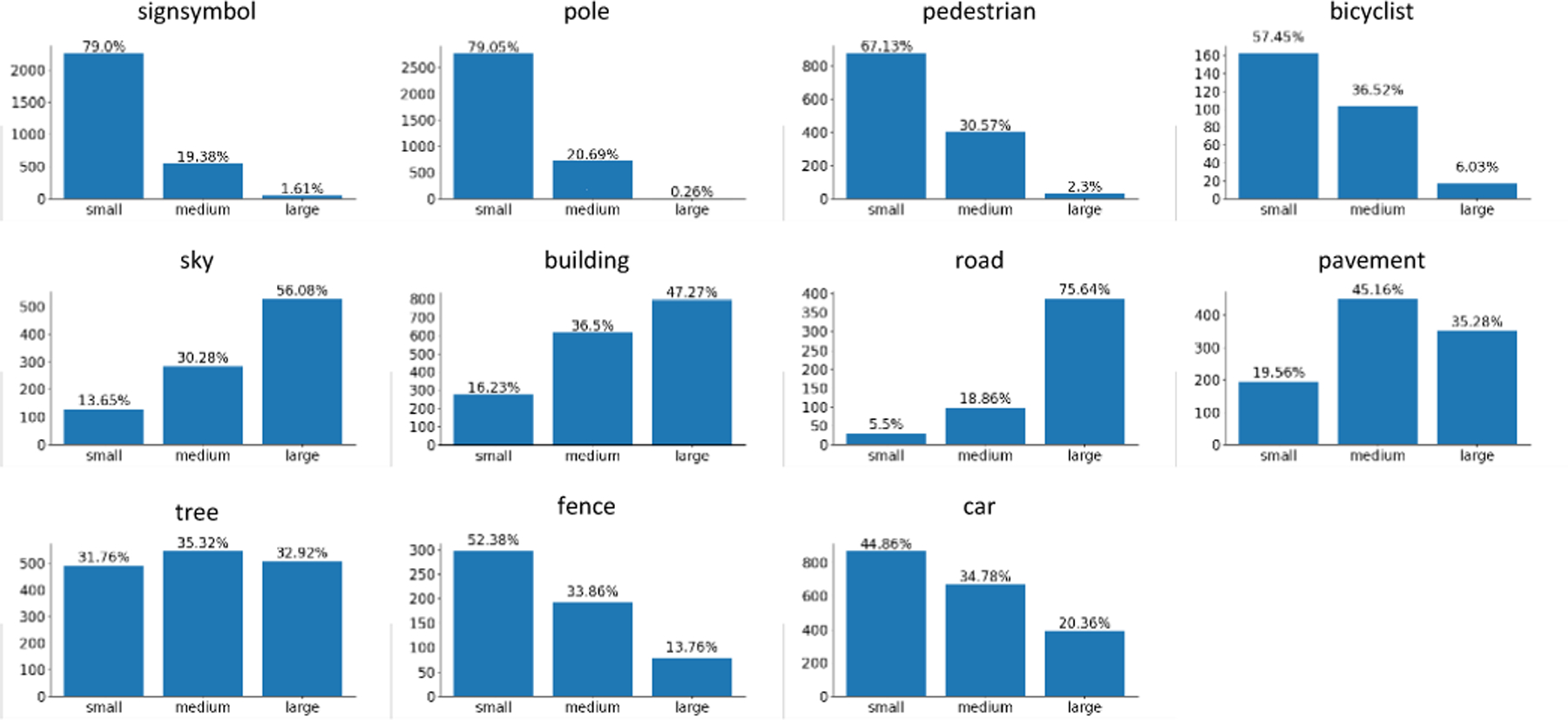
The size distribution of each category of the CamVid training set. The vertical coordinate indicates the number of objects. The small, medium, and large represent the size of an object less than 322 pixels, between 322 and 962 pixels, and larger than 962 pixels, respectively. Detailed image processing and statistical methods are given in the supplementary material.
The performance of AFMA is related to the size distribution of objects and the depth of feature maps. The AFMA depths should be considered when designing models for categories with dominating size distributions. In this study, we only set AFMA at a fixed depth, and developing different AFMA depths for classes with varying distributions is our future work.
4.7. Performance on objects grouped by pixel size
Sec. 4.3 evaluates all models on the small/large objects grouped by object category. However, objects of the large-object category, such as cars, might be shown in small objects at far distances and vice versa. In this section, we evaluate our method on small/large objects grouped by pixel size. All objects are classified as small, medium, and large based on the same criteria adopted in Sec. 4.6. Tab. 4 shows the quantitative results of all models on the Camvid dataset. It demonstrates that the AFMA-based models significantly outperform baseline methods on small object segmentation. For example, DeepLabV3, Unet, Unet++, MaNet, FPN, PAN, LinkNet, and PSPNet obtain 4.0%, 4.0%, 3.2%, 3.8%, 2.8%, 3.4%, 4.1%, and 4.7% improvement after combing AFMA, respectively, on small object segmentation after combining AFMA. The results on Cityscapes and the detailed confusion matrix of all methods is summarized in Supplementary Tab. 4, Supplementary figures 16 and 17, respectively. Tab. 1 and Tab. 4 show similar results: the AFMA could significantly enhance baseline model performance on small objects and a slight improvement on non-small object segmentation, no matter the small/large object definition criteria. This is because the small/large objects grouped by category or pixel size have a similar object distribution. For example, Fig. 9 shows that like the small objects (sign symbol, pole, pedestrian, and bicyclist) defined by category in Sec. 4.3, most sign symbols, poles, pedestrians, and bicyclists are small pixel-size objects. For example, about 80% of sign symbols and poles are less than 322 pixels. And similar to the large objects defined by category, more than 80% of the sky, buildings, roads, and pavements are non-small objects (medium or large). The object size distribution of CamVid’s validation, testing, and CityScape dataset can be found in Supplementary Figures 10 to 15.
TABLE 4.
The comparison results of small/non-small objects grouped by pixel size on the CamVid testing dataset.
| Model Name | Object Size |
||
|---|---|---|---|
| small | medium | large | |
| Deeplabv3 | 14.4 | 36.0 | 84.8 |
| DeepLabV3AFMA | 18.4 (4.0%%↑) | 36.9 (0.9%↑) | 86.1 (1.3%↑) |
|
| |||
| Unet | 15.7 | 35.7 | 84.6 |
| UnetAFMA | 19.7 (4.0%↑) | 38.2 (2.5%↑) | 85.5 (0.9%↑) |
|
| |||
| Unet++ | 17.8 | 36.9 | 84.8 |
| Unet++AFMA | 21.0 (3.2%↑) | 38.9 (2.0%↑) | 85.5 (0.7%↑) |
|
| |||
| MaNet | 14.3 | 34.0 | 83.9 |
| MaNetAFMA | 18.1 (3.8%↑) | 37.1 (3.1%↑) | 85.4 (1.5%↑) |
|
| |||
| FPN | 15.2 | 35.6 | 84.9 |
| FPNAFMA | 18.0 (2.8%↑) | 36.6 (1.0%↑) | 85.4 (0.5%↑) |
|
| |||
| PAN | 13.9 | 34.1 | 84.2 |
| PANAFMA | 17.3 (3.4%↑) | 37.5 (3.4%↑) | 85.9 (1.7%↑) |
|
| |||
| LinkNet | 15.1 | 34.9 | 84.8 |
| LinkNetAFMA | 19.2 (4.1%↑) | 37.0 (2.1%↑) | 85.4 (0.6%↑) |
|
| |||
| PSPNet | 14.7 | 30.1 | 81.0 |
| PSPNetAFMA | 19.4 (4.7%↑) | 32.4 (2.3%↑) | 81.6 (0.6%↑) |
4.8. Negative cases study
According to Tab. 1 and Tab. 2, AFMA improves all small object segmentation performance, but it decreases performance in some large objects such as trees, the sky, and cars. In this section, we present a few negative cases of our method, which may be attributable to the mechanism of AFMA. 1) AFMA’s segmentation of combined categories (e.g., bicyclist = human + bycicle) is not good. Fig. 10a shows that MANet and Unet properly segment the bicyclist in the original image. However, our methods segment the bicyclist as a pedestrian and a car separately. Because the definition of bicyclist in CamVid consists of a pedestrian and a bicycle, a bicycle that appears alone is labeled as “car”. The whole is considered a bicyclist when someone is riding it. Our method computes the AFMA independently for the person and bicycle of the bicyclist, resulting in the model giving the person on the bicycle more similarities to pedestrians and the bicycle more associations to cars. Fig. 10b shows another similar example. Fig. 10a and Fig. 10b show that our method pays more attention to the basic subclasses of a combining category, resulting in the false segmentation of combing categories. Other examples could be found in Supplementary Fig. 7.
Fig. 10.

An illustration of some negative cases of our method, which may be attributable to the mechanism of AFMA. (a) and (b) show examples of the segmentation of bicyclist. (c) Examples of the segmentation of the sky in tree branches. (d) and (e) present examples of false negative results.
2) AFMA loses some local relations and generates locality bias. Fig. 10c shows that the baseline methods segment the sky in the tree branches into trees as same as the groundtruth. After combining AFMA, the models segment the tree branches and the sky separately as tree and sky. It’s because AFMA partitions the tree branches and sky of the original image into different image patches, and AFMA adds extra relations to the image patch containing sky with sky-related feature maps. Supplementary Fig. 7 depicts further examples of this kind.
3) AFMA segments objects in the test set that are not labeled. We found that the inconsistency of the small objects’ groundtruth labels causes some negative cases. For example, as shown in Fig. 10d and Fig. 10e, our method segments the distant small trees and distant small poles, which are not labeled in the testing set. Fig. 11 presents the examples of our method segmenting tiny trees (Fig. 11a), poles (Fig. 11b), and cars (Fig. 11c) in the distance that don’t exist in the groundtruth. It shows our method is effective in recognizing various types of small objects. We provide more such negative examples in the Supplementary material (Fig. 7 and Fig. 8).
Fig. 11.

False predictive examples. (a) and (b) show the segmentation of the distant trees and poles which don’t exist in the groundtruth. (c) Segmenting the small cars that groundtruth doesn’t label.
4.9. Parameter analysis
Since larger models often achieve better results than smaller models in deep learning, we examine the number of parameters in baseline and our models in this section. According to Sec. 3, the AFMA increases performance primarily by computing the relationship of different levels of feature maps of the baseline model’s encoder, which does not contain a significant number of parameters. Tab. 5 and supplementary Tab. 5 present the size of all models, demonstrating that AFMA only increases a small number of parameters for the baseline models.
TABLE 5.
The parameter size and FLOPs. The FLOPs on CamVid is reported on the 720×960.
| Model | #params (M) | Incre (%) | #FLOPs (G) | Incre (%) |
|---|---|---|---|---|
| Deeplabv3 | 58.62 | 0.10 | 566.43 | 2.35 |
| DeepLabV3AFMA | 58.68 | 579.76 | ||
|
| ||||
| Unet | 51.51 | 0.10 | 146.59 | 2.23 |
| UnetAFMA | 51.57 | 159.91 | ||
|
| ||||
| Unet++ | 67.97 | 0.11 | 585.63 | 8.45 |
| Unet++AFMA | 68.03 | 598.01 | ||
|
| ||||
| MaNet | 166.43 | 0.11 | 221.06 | 8.33 |
| MaNetAFMA | 166.49 | 234.39 | ||
|
| ||||
| FPN | 45.10 | 0.09 | 118.99 | 2.26 |
| FPNAFMA | 45.16 | 132.23 | ||
|
| ||||
| PAN | 43.25 | 0.09 | 127.28 | 2.23 |
| PANAFMA | 43.31 | 140.61 | ||
|
| ||||
| LinkNet | 50.17 | 0.04 | 146.51 | 6.03 |
| LinkNetAFMA | 50.23 | 159.83 | ||
|
| ||||
| PSPNet | 48.85 | 0.04 | 433.65 | 7.29 |
| PSPNetAFMA | 48.91 | 450.75 | ||
The increasing percentage of parameters ranges from 0.04% to 0.14%. The highest increase (0.11%) is observed in Unet++AFMA and ManetAFMA on the Cityscapes dataset, while LinkNetAFMA and PSPNetAFMA has the least increment (0.04%). Tab. 5 and Supplementary Tab. 5 show that the models for the CamVid and Cityscapes datasets are the same size since the models used for the two datasets have the same parameter settings (for example, the patch size of their AFMA is all 10 × 10). The results reveal that the improvement of the model is not due to the increase in the model size. The FLOPs of all models are reported in Tab. 5 and Supplementary Tab. 5. The growth of all FLOPs is almost less than 10%. The Unet on Cityscapes has the highest growth of 11.51%, while PAN and Unet on CamVid have the smallest growth rate of 2.3%.
The figure of training convergence (Fig. 12) shows that the mIoU improves as the number of epochs increases. After 300 epochs, the loss of all approaches converges. In conclusion, the increased number of parameters and FLOPs demonstrate that the suggested AFMA could efficiently improve segmentation performance.
Fig. 12.
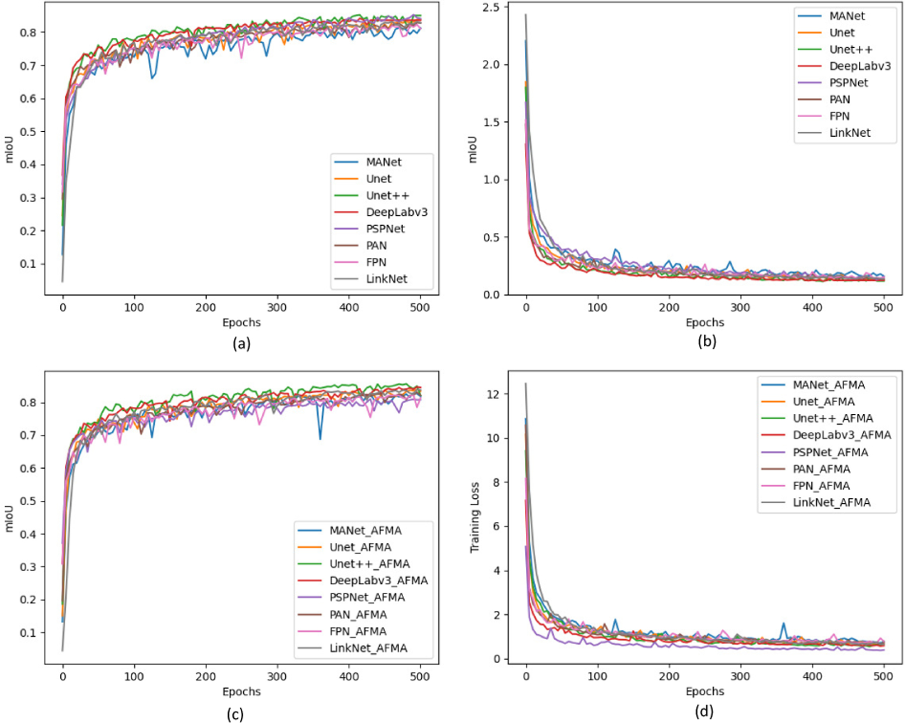
Training convergence. (a) The mIoU of all methods over 500 training epochs on CamVid training dataset. (b) The training loss of all methods over 500 training epochs.
5. Discussion
Why not directly resize the input image to obtain AFMA?
Since the sizes of different objects might be substantially different, our method quantifies the relation between small and large objects by exploiting the original image and its corresponding feature maps. Another more straightforward solution is perhaps to directly resize the original image to a smaller size, then the image patch of the same size can contain larger objects. Similarly, we can also quantify the relation between small and large objects based on the original input and resized images (according to Sec 3.2). However, we empirically find that computing the AFMA via resizing the input image leads to much lower performance than our method. This might be due to that the feature map enjoys larger receptive fields and more enriched semantic information than the image patch (of the same size) from the resized image.
The shape/size of the image/feature patch.
We note that the square image/feature patches can be extended to any shape/size. For example, as shown in Vision Transformer [46] and SwinTransformer [56], the image patch size could be 4×4, 16×16, and 32×32. Furthermore, different categories may favor different patch shape/size. For example, the car category might favor square image/feature patches whereas the column pole object might favor slender rectangle image/feature patches when computing AFMA. We will explore the influence of the size and shape of patches on the segmentation performance in our future work.
What if an image only has one object for a given class?
Our method exploits the relation among objects to compensate for the information loss of the small object. However, in some applications, there may be only one object of a specific type in an image. For example, a CT image often only contains one organ, such as liver, heart, etc. Here we evaluate the models’ performance on objects of each category that individually appear in CamVid and Cityscapes. The results in Supplementary Tab. 6 show that our approach still improves the performance of all the baseline models on small object segmentation. The reason might be that, for the two datasets, only a small number of objects appear individually (the detailed statistics are in Supplementary Tab. 7 and 8). Most images contain more than two objects of the same class, and our method could still learn the relations between categories by other large amounts of co-occur objects. In addition, we tested our method on datasets containing only single object. Interestingly, we empirically find that our method still improves the segmentation performance on liver segmentation (LiTS5), skin lesion (Skin Lesion Analysis Towards Melanoma Detection [57]) and birds (The Caltech-UCSD Birds [58]) datasets. For example, PAN with AFMA improves 1.9% mIoU on skin lesion segmentation, and MaNet with AFMA improves 3.6% mIoU on bird segmentation. The detailed results could be found in Supplementary Tab. 9 and Supplementarty Fig. 9. We believe this is because AFMA can enhance the unrelated relation between the target object and other image patches, therefore eliminating the target object’s false positive prediction.
6. Conclusion
This paper proposes Across Feature Map Attention (AFMA), to improve the performance of existing semantic segmentation models for segmenting small objects. The technique first partitions the original image and its feature maps into image patches of the same size. Then it computes attention between the image patches from various level feature maps to obtain the relations between small and large objects. The obtained attention is used to improve the performance of semantic segmentation. The experiment results show that our method can substantially improve the segmentation accuracy of small objects as well as improve the overall segmentation performance. The proposed method is evaluated based on MaNet, Unet, Unet++, LinkNet, PSPNet, PAN, DeepLabV3, FPN, and other existing small-object segmentation methods on CamVid and Cityscapes. Our method achieves considerable improvement on small object segmentation compared with existing methods. Moreover, we also provide a deeper analysis of the experimental results to better understand the mechanism of AFMA. The proposed AFMA is a lightweight model, which can be easily combined with numerous existing segmentation networks while only incurring neglectable additional training/testing time or expense in deployment.
Supplementary Material
Acknowledgement
This work was partially supported by NIH (1R01CA227713 and 1R01CA256890).
Biographies

Shengtian Sang is currently a post-doctoral scholar at Laboratory of Artificial Intelligence in Medicine and Biomedical Physics in the department of Radiation Oncology at Stanford University. He received the Ph.D. degree with the College of Computer Science and Technology, Dalian University of Technology, Dalian, China. His current research interests are medical data mining, medical image computing, and machine learning. In his Ph.D. study, he worked on biomedical literature-based discovery and data mining.

Yuyin Zhou is currently an Assistant Professor of Computer Science and Engineering at UC Santa Cruz. She received her Ph.D. from the Computer Science Department at Johns Hopkins University in 2020 and was a postdoctoral researcher at Stanford University from 2020 to 2021. Yuyin’s research interests span the fields of medical image computing, computer vision, and machine learning, especially the intersection of them. She has over 20 peer-reviewed publications at top-tier conferences and journals including CVPR, ICCV, AAAI, TPAMI, TMI, MedIA, etc. Yuyin Zhou has led the ICML 2021 workshop on Interpretable Machine Learning in Healthcare, the ICCV 2021 workshop on Computer Vision for Automated Medical Diagnosis, and co-organized ML4H 2021, the 9th CVPR MCV workshop. She served as a senior program committee for IJCAI 2021 and AAAI 2022, an area chair for MICCAI 2022, CHIL 2022.

Md Tauhidul Islam is a post-doctoral scholar at Laboratory of Artificial Intelligence in Medicine and Biomedical Physics In the department of Radiation Oncology at Stanford University. He received the B.Sc. and M.Sc. degrees in electrical and electronic engineering from Bangladesh University of Engineering and Technology (BUET), Dhaka, in 2011 and 2014, respectively. Md Tauhidul Islam is a student member of IEEE. His current research interests are high dimensional medical data analysis using deep learning, manifold embedding and interpretability of deep neural networks. His past research interests were in diverse areas of biomechanics, ultrasound imaging, elastography and signal processing. In his Ph.D. study, he worked on ultrasound elastography at Ultrasound and Elasticity Imaging Laboratory, Department of Electrical Engineering, Texas A&M University.

Lei Xing received the Ph.D. degree in physics from the Johns Hopkins University, Baltimore, MD, USA, in 1992. He completed the Medical Physics Training at The University of Chicago, Chicago, IL, USA. He is currently the Jacob Haimson Sarah S. Donaldson Professor of medical physics and the Director of the Medical Physics Division, Radiation Oncology Department, Stanford University, Stanford, CA, USA. He also holds affiliate faculty positions at the Department of Electrical Engineering, Bio-X and Molecular Imaging Program, Stanford University. He has been a member of the Radiation Oncology Faculty, Stanford University, since 1997. His current research interests include medical imaging, artificial intelligence in medicine, treatment planning, image-guided interventions, nanomedicine, and applications of molecular imaging in radiation oncology.
Footnotes
To make the patch size divisible by the feature map size of , bottom-right padding is employed on the feature map if needed.
Contributor Information
Shengtian Sang, Department of Radiation Oncology, Stanford University, Stanford, CA, USA.
Yuyin Zhou, Department of Computer Science and Engineering at University of California, Santa Cruz, CA, USA.
Md Tauhidul Islam, Department of Radiation Oncology, Stanford University, Stanford, CA, USA.
Lei Xing, Department of Radiation Oncology, Stanford University, Stanford, CA, USA.
References
- [1].Taghanaki SA, Abhishek K, Cohen JP, Cohen-Adad J, and Hamarneh G, “Deep semantic segmentation of natural and medical images: A review,” Artificial Intelligence Review, vol. 54, no. 1, pp. 137–178, 2021. [Google Scholar]
- [2].Long J, Shelhamer E, and Darrell T, “Fully convolutional networks for semantic segmentation,” in Proceedings of the IEEE conference on computer vision and pattern recognition, 2015, pp. 3431–3440. [DOI] [PubMed] [Google Scholar]
- [3].Li X, Zhao H, Han L, Tong Y, Tan S, and Yang K, “Gated fully fusion for semantic segmentation,” in Proceedings of the AAAI conference on artificial intelligence, vol. 34, no. 07, 2020, pp. 11 418–11 425. [Google Scholar]
- [4].Li Y, Huang Q, Pei X, Chen Y, Jiao L, and Shang R, “Cross-layer attention network for small object detection in remote sensing imagery,” IEEE Journal of Selected Topics in Applied Earth Observations and Remote Sensing, vol. 14, pp. 2148–2161, 2020. [Google Scholar]
- [5].Huynh C, Tran AT, Luu K, and Hoai M, “Progressive semantic segmentation,” in Proceedings of the IEEE/CVF Conference on Computer Vision and Pattern Recognition, 2021, pp. 16 755–16 764. [Google Scholar]
- [6].Liu W, Anguelov D, Erhan D, Szegedy C, Reed S, Fu C-Y, and Berg AC, “Ssd: Single shot multibox detector,” in European conference on computer vision Springer, 2016, pp. 21–37. [Google Scholar]
- [7].Hamaguchi R, Fujita A, Nemoto K, Imaizumi T, and Hikosaka S, “Effective use of dilated convolutions for segmenting small object instances in remote sensing imagery,” in 2018 IEEE winter conference on applications of computer vision (WACV). IEEE, 2018, pp. 1442–1450. [Google Scholar]
- [8].Ramos S, Gehrig S, Pinggera P, Franke U, and Rother C, “Detecting unexpected obstacles for self-driving cars: Fusing deep learning and geometric modeling,” in 2017 IEEE Intelligent Vehicles Symposium (IV). IEEE, 2017, pp. 1025–1032. [Google Scholar]
- [9].Meng Z, Fan X, Chen X, Chen M, and Tong Y, “Detecting small signs from large images,” in 2017 IEEE International Conference on Information Reuse and Integration (IRI). IEEE, 2017, pp. 217–224. [Google Scholar]
- [10].Li J, Liang X, Wei Y, Xu T, Feng J, and Yan S, “Perceptual generative adversarial networks for small object detection,” in Proceedings of the IEEE conference on computer vision and pattern recognition, 2017, pp. 1222–1230. [Google Scholar]
- [11].Gupta K, Javed SA, Gandhi V, and Krishna KM, “Mergenet: A deep net architecture for small obstacle discovery,” in 2018 IEEE International Conference on Robotics and Automation (ICRA). IEEE, 2018, pp. 5856–5862. [Google Scholar]
- [12].Li H, Lin Z, Shen X, Brandt J, and Hua G, “A convolutional neural network cascade for face detection,” in Proceedings of the IEEE conference on computer vision and pattern recognition, 2015, pp. 5325–5334. [Google Scholar]
- [13].Chen X, Kundu K, Zhu Y, Berneshawi AG, Ma H, Fidler S, and Urtasun R, “3d object proposals for accurate object class detection,” in Advances in Neural Information Processing Systems Citeseer, 2015, pp. 424–432. [Google Scholar]
- [14].Ronneberger O, Fischer P, and Brox T, “U-net: Convolutional networks for biomedical image segmentation,” in International Conference on Medical image computing and computer-assisted intervention. Springer, 2015, pp. 234–241. [Google Scholar]
- [15].Bansal A, Chen X, Russell B, Gupta A, and Ramanan D, “Pixelnet: Towards a general pixel-level architecture,” arXiv preprint arXiv:1609.06694, 2016. [Google Scholar]
- [16].Hariharan B, Arbela Péz, R. Girshick, and Malik J, “Hyper-columns for object segmentation and fine-grained localization,” in Proceedings of the IEEE conference on computer vision and pattern recognition, 2015, pp. 447–456. [Google Scholar]
- [17].Chen L-C, Papandreou G, Schroff F, and Adam H, “Rethinking atrous convolution for semantic image segmentation,” arXiv preprint arXiv:1706.05587, 2017. [Google Scholar]
- [18].Zhao H, Shi J, Qi X, Wang X, and Jia J, “Pyramid scene parsing network,” in Proceedings of the IEEE conference on computer vision and pattern recognition, 2017, pp. 2881–2890. [Google Scholar]
- [19].Yang M, Yu K, Zhang C, Li Z, and Yang K, “Denseaspp for semantic segmentation in street scenes,” in Proceedings of the IEEE conference on computer vision and pattern recognition, 2018, pp. 3684–3692. [Google Scholar]
- [20].Yu F and Koltun V, “Multi-scale context aggregation by dilated convolutions,” arXiv preprint arXiv:1511.07122, 2015. [Google Scholar]
- [21].Chen L-C, Papandreou G, Kokkinos I, Murphy K, and Yuille AL, “Deeplab: Semantic image segmentation with deep convolutional nets, atrous convolution, and fully connected crfs,” IEEE transactions on pattern analysis and machine intelligence, vol. 40, no. 4, pp. 834–848, 2017. [DOI] [PubMed] [Google Scholar]
- [22].Krä henbühl P and Koltun V, “Efficient inference in fully connected crfs with gaussian edge potentials,” Advances in neural information processing systems, vol. 24, pp. 109–117, 2011. [Google Scholar]
- [23].Chandra S and Kokkinos I, “Fast, exact and multi-scale inference for semantic image segmentation with deep gaussian crfs,” in European conference on computer vision. Springer, 2016, pp. 402–418. [Google Scholar]
- [24].Zheng S, Jayasumana S, Romera-Paredes B, Vineet V, Su Z, Du D, Huang C, and Torr PH, “Conditional random fields as recurrent neural networks,” in Proceedings of the IEEE international conference on computer vision, 2015, pp. 1529–1537. [Google Scholar]
- [25].Guo D, Zhu L, Lu Y, Yu H, and Wang S, “Small object sensitive segmentation of urban street scene with spatial adjacency between object classes,” IEEE Transactions on Image Processing, vol. 28, no. 6, pp. 2643–2653, 2018. [DOI] [PubMed] [Google Scholar]
- [26].Badrinarayanan V, Kendall A, and Cipolla R, “Segnet: A deep convolutional encoder-decoder architecture for image segmentation,” IEEE transactions on pattern analysis and machine intelligence, vol. 39, no. 12, pp. 2481–2495, 2017. [DOI] [PubMed] [Google Scholar]
- [27].Chaurasia A and Culurciello E, “Linknet: Exploiting encoder representations for efficient semantic segmentation,” in 2017 IEEE Visual Communications and Image Processing (VCIP). IEEE, 2017, pp. 1–4. [Google Scholar]
- [28].Xia X and Kulis B, “W-net: A deep model for fully unsupervised image segmentation,” arXiv preprint arXiv:1711.08506, 2017. [Google Scholar]
- [29].Yuan Y, Chen X, and Wang J, “Object-contextual representations for semantic segmentation,” in Computer Vision–ECCV 2020: 16th European Conference, Glasgow, UK, August 23–28, 2020, Proceedings, Part VI 16. Springer, 2020, pp. 173–190. [Google Scholar]
- [30].Fu J, Liu J, Wang Y, Zhou J, Wang C, and Lu H, “Stacked deconvolutional network for semantic segmentation,” IEEE Transactions on Image Processing, 2019. [DOI] [PubMed] [Google Scholar]
- [31].Zhou Z, Siddiquee MMR, Tajbakhsh N, and Liang J, “Unet++: A nested u-net architecture for medical image segmentation,” in Deep learning in medical image analysis and multimodal learning for clinical decision support Springer, 2018, pp. 3–11. [DOI] [PMC free article] [PubMed] [Google Scholar]
- [32].Seo H, Huang C, Bassenne M, Xiao R, and Xing L, “Modified u-net (mu-net) with incorporation of object-dependent high level features for improved liver and liver-tumor segmentation in ct images,” IEEE transactions on medical imaging, vol. 39, no. 5, pp. 1316–1325, 2019. [DOI] [PMC free article] [PubMed] [Google Scholar]
- [33].Çiçek Ö, Abdulkadir A, Lienkamp SS, Brox T, and Ronneberger O, “3d u-net: learning dense volumetric segmentation from sparse annotation,” in International conference on medical image computing and computer-assisted intervention. Springer, 2016, pp. 424–432. [Google Scholar]
- [34].Shah S, Ghosh P, Davis LS, and Goldstein T, “Stacked u-nets: a no-frills approach to natural image segmentation,” arXiv preprint arXiv:1804.10343, 2018. [Google Scholar]
- [35].Zhang X, Xu H, Mo H, Tan J, Yang C, Wang L, and Ren W, “Dcnas: Densely connected neural architecture search for semantic image segmentation,” in Proceedings of the IEEE/CVF Conference on Computer Vision and Pattern Recognition, 2021, pp. 13 956–13 967. [Google Scholar]
- [36].Paszke A, Chaurasia A, Kim S, and Culurciello E, “Enet: A deep neural network architecture for real-time semantic segmentation,” arXiv preprint arXiv:1606.02147, 2016. [Google Scholar]
- [37].Minaee S, Boykov YY, Porikli F, Plaza AJ, Kehtarnavaz N, and Terzopoulos D, “Image segmentation using deep learning: A survey,” IEEE Transactions on Pattern Analysis and Machine Intelligence, 2021. [DOI] [PubMed] [Google Scholar]
- [38].Li H, Xiong P, An J, and Wang L, “Pyramid attention network for semantic segmentation,” arXiv preprint arXiv:1805.10180, 2018. [Google Scholar]
- [39].Fan T, Wang G, Li Y, and Wang H, “Ma-net: A multi-scale attention network for liver and tumor segmentation,” IEEE Access, vol. 8, pp. 179 656–179 665, 2020. [Google Scholar]
- [40].Wang T, Zhang L, Wang S, Lu H, Yang G, Ruan X, and Borji A, “Detect globally, refine locally: A novel approach to saliency detection,” in Proceedings of the IEEE conference on computer vision and pattern recognition, 2018, pp. 3127–3135. [Google Scholar]
- [41].Liu N, Han J, and Yang M-H, “Picanet: Learning pixel-wise contextual attention for saliency detection,” in Proceedings of the IEEE Conference on Computer Vision and Pattern Recognition, 2018, pp. 3089–3098. [Google Scholar]
- [42].Chen Z, Guo C, Lai J, and Xie X, “Motion-appearance interactive encoding for object segmentation in unconstrained videos,” IEEE Transactions on Circuits and Systems for Video Technology, vol. 30, no. 6, pp. 1613–1624, 2019. [Google Scholar]
- [43].Yu C, Wang J, Peng C, Gao C, Yu G, and Sang N, “Learning a discriminative feature network for semantic segmentation,” in Proceedings of the IEEE conference on computer vision and pattern recognition, 2018, pp. 1857–1866. [Google Scholar]
- [44].Hu X, Yang K, Fei L, and Wang K, “Acnet: Attention based network to exploit complementary features for rgbd semantic segmentation,” in 2019 IEEE International Conference on Image Processing (ICIP). IEEE, 2019, pp. 1440–1444. [Google Scholar]
- [45].Zhang X, Wang T, Qi J, Lu H, and Wang G, “Progressive attention guided recurrent network for salient object detection,” in Proceedings of the IEEE Conference on Computer Vision and Pattern Recognition, 2018, pp. 714–722. [Google Scholar]
- [46].Dosovitskiy A, Beyer L, Kolesnikov A, Weissenborn D, Zhai X, Unterthiner T, Dehghani M, Minderer M, Heigold G, Gelly S et al. , “An image is worth 16×16 words: Transformers for image recognition at scale,” arXiv preprint arXiv:2010.11929, 2020. [Google Scholar]
- [47].Brostow GJ, Fauqueur J, and Cipolla R, “Semantic object classes in video: A high-definition ground truth database,” Pattern Recognition Letters, vol. 30, no. 2, pp. 88–97, 2009. [Google Scholar]
- [48].Cordts M, Omran M, Ramos S, Rehfeld T, Enzweiler M, Benenson R, Franke U, Roth S, and Schiele B, “The cityscapes dataset for semantic urban scene understanding,” in Proceedings of the IEEE conference on computer vision and pattern recognition, 2016, pp. 3213–3223. [Google Scholar]
- [49].Deng J, Dong W, Socher R, Li L-J, Li K, and Fei-Fei L, “Imagenet: A large-scale hierarchical image database,” in 2009 IEEE conference on computer vision and pattern recognition. Ieee, 2009, pp. 248–255. [Google Scholar]
- [50].Ladicky L, Russell C, Kohli P, and Torr PH, “Associative hierarchical crfs for object class image segmentation,” in 2009 IEEE 12th International Conference on Computer Vision. IEEE, 2009, pp. 739–746. [Google Scholar]
- [51].Lu H, Fang G, Shao X, and Li X, “Segmenting human from photo images based on a coarse-to-fine scheme,” IEEE Transactions on Systems, Man, and Cybernetics, Part B (Cybernetics), vol. 42, no. 3, pp. 889–899, 2012. [DOI] [PubMed] [Google Scholar]
- [52].Tighe J and Lazebnik S, “Superparsing: scalable nonparametric image parsing with superpixels,” in European conference on computer vision. Springer, 2010, pp. 352–365. [Google Scholar]
- [53].Liu B and He X, “Multiclass semantic video segmentation with object-level active inference,” in Proceedings of the IEEE conference on computer vision and pattern recognition, 2015, pp. 4286–4294. [Google Scholar]
- [54].Li X, Jie Z, Wang W, Liu C, Yang J, Shen X, Lin Z, Chen Q, Yan S, and Feng J, “Foveanet: Perspective-aware urban scene parsing,” in Proceedings of the IEEE International Conference on Computer Vision, 2017, pp. 784–792. [Google Scholar]
- [55].Lin T-Y, Maire M, Belongie S, Hays J, Perona P, Ramanan D, Dollár P, and Zitnick CL, “Microsoft coco: Common objects in context,” in European conference on computer vision. Springer, 2014, pp. 740–755. [Google Scholar]
- [56].Liu Z, Lin Y, Cao Y, Hu H, Wei Y, Zhang Z, Lin S, and Guo B, “Swin transformer: Hierarchical vision transformer using shifted windows,” arXiv preprint arXiv:2103.14030, 2021. [Google Scholar]
- [57].Codella NC, Gutman D, Celebi ME, Helba B, Marchetti MA, Dusza SW, Kalloo A, Liopyris K, Mishra N, Kittler H et al. , “Skin lesion analysis toward melanoma detection: A challenge at the 2017 international symposium on biomedical imaging (isbi), hosted by the international skin imaging collaboration (isic),” in 2018 IEEE 15th international symposium on biomedical imaging (ISBI 2018). IEEE, 2018, pp. 168–172. [Google Scholar]
- [58].Wah C, Branson S, Welinder P, Perona P, and Belongie S, “The caltech-ucsd birds-200–2011 dataset,” 2011. [Google Scholar]
Associated Data
This section collects any data citations, data availability statements, or supplementary materials included in this article.