

Abstract

This research focuses on an inclined curved crack model for a recycled aluminum composite beam at various crack depths and locations. The inclined curved crack equation of the motion, by governing a free vibration curved beam with a different depth of crack, is solved computationally via the differential quadrature method (DQM) and experimentally; additionally, the result of the natural frequency has been compared with various depths of curvature. For the first four modes of cracked beams, the computational method’s output is used to determine the natural frequencies associated with mode shapes. The outcomes of the computational results suggested a structural health monitoring system to detect deterioration in composite structures when modal parameters have changed. An experimental set of results was validated using MATLAB2019a, and the outcomes were compared with an artificial neural network.
1. Introduction
Due to their outstanding qualities, such as their light weight, high ratio strength, stiffness, and design flexibility, curved composite structures are now widely used in the aerospace industry.1,2 The primary structural components for the new formation of wide-body airplanes are rapidly shifting toward material composites. Structures impulsively loaded with high pressures to the point of breakage represent a significant class of concerns in safety and security.3 Furthermore, the transition zone between an aircraft’s wing beam and the web is where the curved composite construction is most frequently used. However, geometry shape, structural complexity, and curved composite constructions are easily stressed and carry a heavy load.4,5 The physical characteristics of the curve structure change as a result of damage, which has an impact on real-time application. It must be identified early to avoid catastrophic failure and prolong the life of the mechanical system.
Composite materials frequently employed in aerospace and aeronautical engineering to reduce weight have been studied. The major benefits of composite materials are high specific stiffness, strength, and corrosion resistance. However, these materials are incredibly prone to deterioration or cracking.6−8 Effective dynamic behavior forecasting is essential exclusively for structures exposed to dynamic loads. The natural frequency may be influenced by various factors, including the beam’s curvature, end circumstances, beam shape, cross-sectional form, etc. To effectively estimate a structure’s natural frequency, it is necessary to determine how each parameter affects it.9−11
Many academics have been drawn to studying curved beams for many years. A comprehensive analysis of the free vibration research of curved beams has been provided by Chidamparam and Leissa.12 Most of the article provides a nonexhaustive collection of research studies on the free in-plane and out-of-plane vibration of curved beams. Axial extensibility, rotary inertia, and shear deformation were considered for the curved beam structure.13,14 A precise solution is found for the free vibration issue in the curved beam.15,16 With the advent of new technologies came an increase in the use of the FEM, which made it even more easier to resolve the free vibration issue in complex structures.17−19 Rabczuk et al.20−22 have described the mesh-free method of dynamic fracture of complex geometric structures of nonlinearities, and it will give better results in multiple crack models. In most structural model studies, the prediction of natural frequencies, the dynamic stability assessment of curved beams using a system of spring mass, and studies of in-plane and out-of-plane vibration of straight and curved stepped beams are used for FEM of curved beams.23,24 The static stability of curved cracked beams was the main focus of early studies. FEM and analytical approaches have been used to study the static behavior of curved beams with different boundary conditions. However, vibrational problems are distinct from static issues. Vibration has positive and negative effects on structures.25 To investigate vibration problems with curved beams, some vibration analysis approaches have been developed.26
Due to their small weight, beams are frequently employed in engineering and mechanics. In engineering practice, mechanical analysis is essential. The mechanical structure is most important in practical engineering applications. Due to the limitations of the analytical method, especially in solving a curved crack beam, a variety of numerical methods have been developed using the finite element method,27 transfer matrix method,28 differential quadrature method,29 meshfree30,31 isogeometric analysis,32,33 meshless method,34,35 and, recently, deep learning-based methods.36−38
The DQM, which uses a very small number of grid points to solve partial differential equations (PDE), was first suggested by Bellman and Casti39 in 1971. Numerous studies have helped to create and apply the most effective approach of DQM,40−44 which is regarded as a good alternative to traditional numerical methods like the FEM. The conventional DQM is inappropriate for issues involving unstable regions and discontinuities.45,46 This class belongs to the generalized differential quadrature (GDQ) method, which reduces arbitrary-order derivatives as the weighted sum of the values the unknown function assumes on a discrete computing grid.47,48 Additionally, it has been successfully used in contact applications and fracture mechanics problems.
Artificial neural networks (ANN) are a popular example of soft computing technology these days. Researchers are now turning to machine learning approaches to accurately forecast the results of complex engineering challenges. It is used in a variety of fields, such as structural engineering,49−52 construction management project decision-making,53,54 mechanical engineering problem-solving, and several concrete technology-related issues. However, there are many examples of it being used in structural dynamics research. Few studies have examined the free vibration response of angle ply laminates55,70,71 or the effects of dimensions like length, thickness, and breadth on the dynamic response of single- and multistepped beams.56,72 Sahin and Shenoi57 described ANN as the most efficient method for vibration data analysis for the severity of damage and location detection on the cantilever beam. Simulate neural networks has predicated the one hidden layer are describe on MATLAB2019 using a neural network toolbox. The neural networks present here are used to forecast the location and severity of damage to different crack locations. The four-mode shapes are the same, and the location is used to predict the accuracy. Raja et al.58 have described a back-propagation neural network designed to estimate the magnitude of the crack damage and crack location.
This article is organized as follows: Section 1 presents the main idea and an overview of the related studies on the research study of literature surveys. In Section 2, the theoretical formulations are developed in detail for curved crack beams. Section 3 expands the computation method of the differential quadrature method of the curved crack beam. Section 4 explains the fabrication of recycled aluminum composite beams and the experimental analysis of the curved crack beam. The results and discussion Section 5 compare the DQM vs experimental study along different mode shapes and curvatures. The predation of the ANN with a hidden layer of the squeeze and excitation method and a summary of some of the experimental results are included, which also presents the conclusion of this study.
2. Curved Beam Equation
Kundu and Sinha63 provide nonlinear strain–displacement relationships for any three-dimensional elastic body in the orthogonal curvilinear coordinate system α1α2ξ. According to Zhibo et al.40 assuming zero displacement in the α2 direction (v = 0), nonlinear longitudinal strain in the α1 direction (ε11) and shear strain in 1–3 planes (γ13) are expressed as eqs 1 and 2
| 1 |
| 2 |
When the radius of curvature is constant, e11, e31, and e13 are given as 3–5
| 3 |
| 4 |
| 5 |
Here, u and w denote displacements, respectively, in the a1 and ζf directions. R1 indicates the principal radius of curvature in the a1–ζ plane.
The curvilinear coordinate system of the curved crack composites beam is notated simply hereafter; the crack depth angle is θ, the inclined crack angle is 45°, the width is b, hc and subscript of radius of curvature R. Figure 1a,b displays the fundamental characteristics of a curved beam.
Figure 1.

(a) Inclined curved crack beam and (b) curved beam parameter.
A point (x, y) at time t can stand as the starting point for rotating and midplane displacement in the curved beam displacement of eqs 6 and 7:
| 6 |
| 7 |
where θx is the rotation about the y-axis and u0 and w0 are midplane displacements.
When replacing eqs 8 and 9 in 1, the following Green–Lagrange nonlinear strain–displacement relationship has been identified for curved crack beams:
| 8 |
| 9 |
where εi and εsi are given as eqs 10–17
| 10 |
| 11 |
| 12 |
| 13 |
| 14 |
| 15 |
| 16 |
| 17 |
No assumptions or simplifications are used in the derivation of the nonlinear relationship.
The constitutive equation for a curved crack beam can be written as when it is defined in terms of in-plane force and moment resultants in eq 18:
 |
18 |
As a result of the shear force resultant, the laminate composition equation for transverse shear is stated as eq 19:
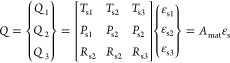 |
19 |
The laminated stiffness coefficients Ti,Pi, Ri, Di, Ei, Tsi, Psi, and Rsi stand for in-plain, bending stretching coupling, bending, and transverse shear stiffness. They are acquired as shown below eq 20–35:
| 20 |
| 21 |
| 22 |
| 23 |
| 24 |
| 25 |
| 26 |
| 27 |
| 28 |
| 29 |
| 30 |
| 31 |
| 32 |
| 33 |
| 34 |
| 35 |
The shear correction factor Ks = 5/6. The corresponding elastic modulus is given as E(k)x in eq 36
| 36 |
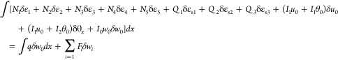
The sum of internal and external forces and the virtual work of external forces can be the starting point for a dynamic form of the virtual work principle. It is possible to write deeply curved in the absence of dampening as 37
 |
37 |
The distribution load q(x, t) equation can expressed as follows by multiplying the load amplitude qx(x) by the pulse function p(t), as expressed in eq 38
| 38 |
The left side of the equation’s first term group represents the theoretical work of internal forces brought on by stress, while the second term group represents the theoretical work of inertia forces brought on by acceleration. The virtual work of concentered forces and external forces arises from distribution load.
Equation 39 can be expressed as follows using force, moment resultants, and mass inertia.
| 39 |
Similar to how the load amplitude Pc and pulse function can be combined, the concentrated force Fi(t) can be expressed as follows.
The first group of terms in the equation illustrates the virtual work done by inertia forces caused by accelerations. Due to distribution load, the first term on the right shows the virtual work of external forces, while the second term shows the virtual work below 40 and 41:
 |
40 |
I0, I1, and I2 are given as
| 41 |
where ρ(k) denotes the density of the kth layer.
The following matrix can be constructed by utilizing the virtual work equation in the equation of motion eq 42:
| 42 |
where F, Ü, and P stand for exterior forces, internal forces, and acceleration, respectively, and M is the mass matrix. The implicit new mark constant average acceleration time integration scheme has been demonstrated in eq 43, and it may be used to determine the transient response for the curved beam:
| 43 |
After formulating acceleration in terms of an unknown displacement, the residual equation is linearized, resulting in the incremental equilibrium shown in eq 44 below:
| 44 |
The result of the equation’s solution is incremental displacement. Final values are produced by adding displacement increments to the earlier values.
The V matrix in the eq 45 is often referred to as the tangent stiffness matrix and curved beam
| 45 |
where Bb, Bs, Qp, Np, and Nd are given as eqs 46–49:
 |
46 |
 |
47 |
 |
48 |
 |
49 |
Utilizing numerical integration, the tangent stiffness matrix is calculated and the Nd matrix for the ith integration points Nid is given as eq 50:
 |
50 |
3. Differential Quadrature Method
The DQM, a modified version of GDQM, is used in this study to determine the positional derivatives of the field factors in eq 40. The curved crack beam is discretized using grid points before applying DQM to identify the regions where derivative and field value variables are to be calculated, as shown in Figure 2.
Figure 2.

Grid points on a curved beam.
The derivative of a function relating to a variable at a specific discrete location can be expressed using DQM as a weighted linear sum of the values of the process at all of the individual areas along the mesh line. The selection of crack location, depth of crack, quantity of grid points, and computation weight coefficients have a significant impact on the exact DQM. Weight coefficients were determined using a flawed Vandermonde-type algebraic equation system. Formulation of DQM by Bellman et al.65 prevents the usage of significant grid numbers. Shu developed the generalized differential quadrature method (GDQM) for determining the weight coefficients for first-order and higher-order derivatives with any number and distribution of grid points. The implementation of the Shu technique to solve various technical challenges was quite flexible. With the generalized differential quadrature method (GDQ), the rth order derivative of a function f(x) with n discrete grid points can be expressed as higher-order derivatives with any number and distribution of grid points, as shown in eq 51. Shu’s method provided a great deal of versatility in how the method can be applied to tackle different engineering challenges.67,68
| 51 |
where xi represents different points in the variable region, and fj and C(r)ij are the function values and related weighting coefficients, respectively.
The weight coefficients C(r)ij in DQM are calculated by using Lagrange polynomial functions. For the first-order derivative, i.e., r = 1, the explicit formula for the weight coefficients of DQM is as follows (eqs 52 and 53):
| 52 |
where
| 53 |
The following recursive relations can be used for higher-order derivations (eqs 54 and 55):
| 54 |
 |
55 |
In terms of choosing grid points, the GDQ approach does not impose any limitations. As a result, the grid points are chosen as Gauss–Lobatto points. Equation 40 uses these points for integral quadrature as well. When the GDQ method is used to calculate derivatives, the Lobatto rule produces grid points with irregular intervals. Additionally, it adds grid points to the boundaries, making it easier to apply boundary constraints.
The grid points of the Lobatto nonuniform system in polar space (−1 ≤ ξi ≤ 1) are given below 56
| 56 |
where ξi(i = 2, ..., n – 1) corresponds to the (i – 1)th zero, as shown in eq 57
| 57 |
where Pn–1(ξ) is a legend polynomial of the (n – 1)th order.
4. Results and Discussion
4.1. Fabrication Method
Silicon carbide (SiC) metal powder was purchased from Sigma-Aldrich, India. In this study, a gradient composite constructed of aluminum alloy scraping chips (05 wt % SiC) was produced in two steps—ball milling and die casting—and has an outer radius and thickness of 60 and 30 mm, respectively. With the aid of an annular furnace, the SiC particles were heated to 600 C for 2 h to remove moisture, which improves their wettability with the molten metal. According to Ashok and Prases K M,69 ethanol was used to clean aluminum alloy chips and get rid of dust, as shown in Figure 3.
Figure 3.

Balling milling.
The mechanical stirrer was used to guarantee that the SiC particles (solid phase) were uniformly dispersed throughout the metal matrix for 15 min at 250 rpm when the chips reached the molten stage (soft phase), following the completion of balling for 6 h. The 725 °C molten metal was finally poured into the 1200 rpm revolving centrifugal casting mold, allowed to solidify, and then shaped into the curved beam, as illustrated in Table 1, by its mechanical characteristics and geometrical characteristics. The values for the mechanical properties are provided in Table 2.
Table 1. Properties of the Curved Beam.
| s. no | property | notation | value |
|---|---|---|---|
| 1 | radius of the beam axis | R | 80 mm |
| 2 | opening angle of the beam | θ | 119° |
| 3 | height of the cross section | h | 6 mm |
| 4 | inclined crack angle | ϕ | 45° |
| 5 | beam of the cross section | b | 20 mm |
| 6 | Young’s modulus | E | 115 GPa |
| 7 | Poisson’s ratio | v | 0.33 |
| 8 | density | γ | 2.73 |
Table 2. Mechanical Properties of Aluminum, Recycled Aluminum, and Aluminum Metal Matrix Composites.
| s. no | mechanical properties | units | aluminum | recycled aluminum | recycled aluminum + SiC |
|---|---|---|---|---|---|
| 1 | Vickers hardness | VHS | 24 | 23 | 38 |
| 2 | tensile strength | Mpa | 28.45 | 27.54 | 58.35 |
The hardness value increases with the percentage increase of SiC. The decrease in the strength and hardness with the increase of metal matrix composites with increase of SiC maybe attributed to increase in porosity as the silicon carbide.
4.2. Experimental Method
Some experimental tests were conducted on a specimen with mechanical characteristics to determine the natural frequency and mode shapes, which are listed in Table 1 (note that all of the results in the following section were obtained using a beam with these mechanical properties). Rubber bands of low stiffness are utilized to hang the beam from a stationary frame, ensuring that it will not be subjected to stress from the support outside a safety margin.
Therefore, it is assumed that the beam can move freely. The experiments are run four times: the first time on an undamaged beam to assess mode shapes and the remaining three times with cracks inserted at relative depths of 0.1, 0.2, 0.3, 0.4, and 0.5 to determine the natural frequencies. The relative depth and position of the damage are defined by the ratio of the depth of the crack to the cross-sectional height and the angle of the fracture to the overall angle of the beam. The tests are run using an impulsive approach. Figure 4 shows a computer, hammer, and other commonplace tools the Danish company Bruel and Kjaer produced.
Figure 4.

Vibrational analysis of the experimental setup.
4.3. Deflection in the Vibration Mode
Dahak et al.66 have described the natural frequency as the biggest drawback if the damage location is symmetrical to one of the mode shapes. In the natural frequency of this mode, the mode remains unchanged. In this cross section, the report has to give more accuracy of different damage locations. One of the most common disadvantages of natural frequency is when the damage is lower than that of the mode shape. The frequency of this mode remains unchanged in this case. The results in this section are more accurate.
The vibrational behavior of specimen damage and the undamaged beam of the cantilever beam of relative natural frequency are shown in Figure 5. As shown in the flowchart, the relative natural frequency of modes (i = 1, 2, 3, 4) is equal to the ratio of natural frequency of the damage beam fidamage to the natural frequency of the free undamaged beam fiundamaged. The relative natural frequency for different crack locations of crack depth (0.1, 0.2, 0.3, 0.4, 0.5).
Figure 5.

Flowchart of relative natural frequency.
A new method of induced relative natural frequency for different cracks and different crack depths was developed. The damage in different crack locations in the beam has been determined in various research articles. The damage present in the structure of the relative natural frequency is as follows.
Stage 1 – Give the first four frequencies of damage and undamaged structure.
Stage 2 – Find out the relative natural frequency
Stage 3 – In fine feather induced relative natural frequency differs from undamaged, therefore presence in the damage structure.
Stage 4 – Verify that the normal frequency is equal to 1. The flowchart prospects the method of natural frequency with different crack locations.
As would be expected, the value of the natural frequencies steadily decreases as the depth of the fracture increases, as clearly visible in Figure 6a,b, with different depths of the crack. Since the relationship between beam stiffness and fracture crack depth is direct, increasing the crack depth would cause the beam’s stiffness to decrease in DQM, which would lower the relative natural frequency, as shown in Table 3.
Figure 6.

(a,b) First mode shape of DQM and experimental method.
Table 3. First Mode Shape Relative Natural Frequency of Experimental Method v DQM.
| experimental
method |
DQM |
||||||||||
|---|---|---|---|---|---|---|---|---|---|---|---|
| s. no | relative crack location (m) | 0.1 | 0.2 | 0.3 | 0.4 | 0.5 | 0.1 | 0.2 | 0.3 | 0.4 | 0.5 |
| 1 | 1 | 0.9964 | 0.9736 | 0.9509 | 0.9281 | 0.9053 | 0.9965 | 0.9735 | 0.9508 | 0.9280 | 0.9052 |
| 2 | 2 | 0.9966 | 0.9746 | 0.9528 | 0.9309 | 0.909 | 0.9966 | 0.9745 | 0.9525 | 0.9311 | 0.9098 |
| 3 | 3 | 0.9967 | 0.9758 | 0.9551 | 0.9343 | 0.9135 | 0.9967 | 0.9757 | 0.9552 | 0.9345 | 0.9136 |
| 4 | 4 | 0.9969 | 0.9767 | 0.9566 | 0.9366 | 0.9165 | 0.9969 | 0.9768 | 0.9567 | 0.9368 | 0.9167 |
| 5 | 5 | 0.9971 | 0.9778 | 0.9587 | 0.9396 | 0.9205 | 0.9971 | 0.9779 | 0.9589 | 0.9398 | 0.9207 |
| 6 | 6 | 0.9972 | 0.979 | 0.9609 | 0.9427 | 0.9245 | 0.9973 | 0.9792 | 0.961 | 0.9428 | 0.9247 |
| 7 | 7 | 0.9973 | 0.9804 | 0.9634 | 0.9465 | 0.9295 | 0.9974 | 0.9805 | 0.9634 | 0.9466 | 0.9296 |
| 8 | 8 | 0.9974 | 0.9812 | 0.9649 | 0.9487 | 0.9324 | 0.9975 | 0.9814 | 0.9651 | 0.9489 | 0.9325 |
| 9 | 9 | 0.9975 | 0.9817 | 0.9659 | 0.95 | 0.9342 | 0.9976 | 0.9819 | 0.9661 | 0.9505 | 0.9344 |
| 10 | 10 | 0.9976 | 0.9825 | 0.9675 | 0.9524 | 0.9F3 | 0.9977 | 0.9824 | 0.9676 | 0.9531 | 0.9375 |
| 11 | 11 | 0.9977 | 0.9833 | 0.9689 | 0.9545 | 0.9401 | 0.9978 | 0.9835 | 0.9691 | 0.9546 | 0.9392 |
| 12 | 12 | 0.9978 | 0.9842 | 0.9705 | 0.9569 | 0.9432 | 0.9979 | 0.9843 | 0.9702 | 0.9572 | 0.9431 |
| 13 | 13 | 0.9979 | 0.9851 | 0.9724 | 0.9596 | 0.9468 | 0.9979 | 0.9852 | 0.9725 | 0.9598 | 0.9468 |
| 14 | 14 | 0.9979 | 0.9857 | 0.9736 | 0.9614 | 0.9492 | 0.998 | 0.9857 | 0.9737 | 0.9615 | 0.9486 |
| 15 | 15 | 0.998 | 0.9865 | 0.975 | 0.9634 | 0.9519 | 0.9981 | 0.9866 | 0.9752 | 0.9635 | 0.9521 |
| 16 | 16 | 0.9981 | 0.9874 | 0.9767 | 0.9659 | 0.9552 | 0.9982 | 0.9875 | 0.9768 | 0.9662 | 0.9553 |
| 17 | 17 | 0.9982 | 0.9882 | 0.9783 | 0.9683 | 0.9583 | 0.9983 | 0.9883 | 0.9785 | 0.9685 | 0.9584 |
| 18 | 18 | 0.9982 | 0.9887 | 0.9792 | 0.9697 | 0.9602 | 0.9983 | 0.9887 | 0.9794 | 0.9698 | 0.9603 |
| 19 | 19 | 0.9983 | 0.9896 | 0.9809 | 0.9722 | 0.9635 | 0.9984 | 0.9897 | 0.9812 | 0.9724 | 0.9634 |
| 20 | 20 | 0.9984 | 0.9904 | 0.9823 | 0.9743 | 0.9662 | 0.9985 | 0.9905 | 0.9825 | 0.9744 | 0.9664 |
| 21 | 21 | 0.9985 | 0.9911 | 0.9836 | 0.9762 | 0.9687 | 0.9986 | 0.9913 | 0.9837 | 0.9765 | 0.9689 |
| 22 | 22 | 0.9986 | 0.9915 | 0.9845 | 0.9774 | 0.9703 | 0.9987 | 0.9916 | 0.9848 | 0.9776 | 0.9712 |
| 23 | 23 | 0.9986 | 0.9925 | 0.9865 | 0.9804 | 0.9743 | 0.9988 | 0.9928 | 0.9867 | 0.9805 | 0.9748 |
| 24 | 24 | 0.9987 | 0.9936 | 0.9885 | 0.9834 | 0.9783 | 0.9989 | 0.9937 | 0.9886 | 0.9835 | 0.9787 |
| 25 | 25 | 0.9988 | 0.9942 | 0.9896 | 0.985 | 0.9804 | 0.999 | 0.9943 | 0.9898 | 0.9854 | 0.9806 |
| 26 | 26 | 0.9989 | 0.9948 | 0.9908 | 0.9867 | 0.9826 | 0.9991 | 0.9948 | 0.9909 | 0.9868 | 0.9827 |
| 27 | 27 | 0.999 | 0.9952 | 0.9914 | 0.9875 | 0.9837 | 0.9992 | 0.9953 | 0.9915 | 0.9876 | 0.9838 |
| 28 | 28 | 0.9991 | 0.9954 | 0.9917 | 0.9879 | 0.9842 | 0.9993 | 0.9956 | 0.9918 | 0.9879 | 0.9845 |
| 29 | 29 | 0.9992 | 0.9957 | 0.9922 | 0.9886 | 0.9851 | 0.9993 | 0.9958 | 0.9922 | 0.9886 | 0.9852 |
| 30 | 30 | 0.9993 | 0.996 | 0.9928 | 0.9895 | 0.9862 | 0.9994 | 0.9962 | 0.9931 | 0.9896 | 0.9862 |
| 31 | 31 | 0.9994 | 0.9964 | 0.9933 | 0.9903 | 0.9872 | 0.9994 | 0.9965 | 0.9934 | 0.9904 | 0.9873 |
| 32 | 32 | 0.9995 | 0.9968 | 0.9941 | 0.9913 | 0.9886 | 0.9995 | 0.9968 | 0.9942 | 0.9914 | 0.9886 |
| 33 | 33 | 0.9996 | 0.9975 | 0.9953 | 0.9932 | 0.991 | 0.9996 | 0.9974 | 0.9954 | 0.9934 | 0.9912 |
| 34 | 34 | 0.9997 | 0.9979 | 0.9964 | 0.9948 | 0.9932 | 0.9997 | 0.9978 | 0.9965 | 0.9949 | 0.9933 |
| 35 | 35 | 0.9998 | 0.9986 | 0.9974 | 0.9961 | 0.9949 | 0.9997 | 0.9987 | 0.9975 | 0.9962 | 0.9949 |
| 36 | 36 | 0.9998 | 0.999 | 0.9982 | 0.9975 | 0.9967 | 0.9998 | 0.999 | 0.9983 | 0.9976 | 0.9968 |
| 37 | 37 | 0.9999 | 0.9996 | 0.9993 | 0.9991 | 0.9988 | 0.9998 | 0.9996 | 0.9993 | 0.9992 | 0.9987 |
| 38 | 38 | 0.9999 | 0.9999 | 0.9999 | 0.9999 | 0.9999 | 0.9999 | 0.9998 | 0.9999 | 0.9999 | 0.9999 |
| 39 | 39 | 0.9999 | 0.9999 | 1 | 1 | 1 | 0.9999 | 0.9999 | 1 | 1 | 1 |
| 40 | 40 | 1 | 1 | 1 | 1 | 1 | 1 | 1 | 1 | 1 | 1 |
Figure 7a,b shows how crack depth affects relative natural frequencies. Similarly, it illustrates the impact of cracking’s position. These graphs show the second relative natural frequencies for the curved crack beam that has undergone five crackings at relative depths of 0.1, 0.2, 0.3, 0.4, and 0.5. DQEM, and the experimental method is used to collect the data for the diagrams. Recall that the relative frequency is calculated by dividing the natural frequency of the undamaged beam by the natural frequency of the curved broken beam, as shown in Table 4.
Figure 7.

(a, b) Second Mode shape of DQM and experimental method.
Table 4. Second Mode Shape Relative Natural Frequency of Experimental Method v DQM.
| experimental
method |
DQM |
||||||||||
|---|---|---|---|---|---|---|---|---|---|---|---|
| s. no | relative crack location (m) | 0.1 | 0.2 | 0.3 | 0.4 | 0.5 | 0.1 | 0.2 | 0.3 | 0.4 | 0.5 |
| 1 | 1 | 0.9901 | 0.9796 | 0.9691 | 0.9586 | 0.9481 | 0.9907 | 0.9798 | 0.9698 | 0.9598 | 0.9485 |
| 2 | 2 | 0.9915 | 0.9817 | 0.9719 | 0.9621 | 0.9523 | 0.9918 | 0.9821 | 0.9725 | 0.9634 | 0.9534 |
| 3 | 3 | 0.9927 | 0.9838 | 0.9748 | 0.9659 | 0.957 | 0.9931 | 0.9841 | 0.9752 | 0.9662 | 0.9582 |
| 4 | 4 | 0.9939 | 0.9869 | 0.9799 | 0.973 | 0.966 | 0.9952 | 0.9872 | 0.9825 | 0.9764 | 0.9668 |
| 5 | 5 | 0.9952 | 0.9907 | 0.9861 | 0.9816 | 0.9771 | 0.9953 | 0.9929 | 0.9852 | 0.9828 | 0.9778 |
| 6 | 6 | 0.9965 | 0.9948 | 0.993 | 0.9913 | 0.9895 | 0.9972 | 0.9956 | 0.9982 | 0.9929 | 0.9562 |
| 7 | 7 | 0.9977 | 0.997 | 0.9964 | 0.9957 | 0.995 | 0.9983 | 0.9978 | 0.9955 | 0.9962 | 0.9969 |
| 8 | 8 | 0.9984 | 0.9985 | 0.9986 | 0.9987 | 0.9988 | 0.9989 | 0.9991 | 0.9992 | 0.9993 | 0.9978 |
| 9 | 9 | 0.9996 | 0.9997 | 0.9998 | 0.9998 | 0.9999 | 0.9998 | 0.9985 | 0.9989 | 0.9999 | 0.9995 |
| 10 | 10 | 0.9999 | 0.9999 | 0.9999 | 0.9999 | 0.9999 | 0.9999 | 0.9999 | 1 | 1 | 1 |
| 11 | 11 | 0.9992 | 0.9987 | 0.9982 | 0.9977 | 0.9972 | 0.9995 | 0.9989 | 0.9995 | 0.9986 | 0.9963 |
| 12 | 12 | 0.9977 | 0.9956 | 0.9936 | 0.9915 | 0.9895 | 0.9985 | 0.9964 | 0.9943 | 0.9924 | 0.9884 |
| 13 | 13 | 0.9959 | 0.99 | 0.984 | 0.9781 | 0.9721 | 0.9953 | 0.9962 | 0.9849 | 0.9794 | 0.9727 |
| 14 | 14 | 0.9942 | 0.9862 | 0.9782 | 0.9702 | 0.9622 | 0.9947 | 0.9864 | 0.9792 | 0.9725 | 0.9637 |
| 15 | 15 | 0.9931 | 0.9841 | 0.9751 | 0.9662 | 0.9572 | 0.9935 | 0.9847 | 0.9762 | 0.9675 | 0.9586 |
| 16 | 16 | 0.9922 | 0.9822 | 0.9722 | 0.9621 | 0.9521 | 0.9928 | 0.9832 | 0.9738 | 0.9634 | 0.9534 |
| 17 | 17 | 0.9912 | 0.9809 | 0.9705 | 0.9602 | 0.9498 | 0.9923 | 0.9817 | 0.9715 | 0.9615 | 0.9509 |
| 18 | 18 | 0.9903 | 0.979 | 0.9677 | 0.9565 | 0.9452 | 0.9912 | 0.9798 | 0.9682 | 0.9567 | 0.9464 |
| 19 | 19 | 0.9898 | 0.9777 | 0.9655 | 0.9534 | 0.9412 | 0.9888 | 0.9782 | 0.9661 | 0.9542 | 0.9426 |
| 20 | 20 | 0.9894 | 0.9771 | 0.9647 | 0.9524 | 0.94 | 0.9895 | 0.9775 | 0.9662 | 0.9535 | 0.9413 |
| 21 | 21 | 0.9893 | 0.9767 | 0.9641 | 0.9515 | 0.9389 | 0.9896 | 0.9772 | 0.9653 | 0.9519 | 0.9402 |
| 22 | 22 | 0.9895 | 0.9768 | 0.9641 | 0.9515 | 0.9388 | 0.9894 | 0.9769 | 0.9644 | 0.9525 | 0.9389 |
| 23 | 23 | 0.9905 | 0.9783 | 0.9661 | 0.9539 | 0.9416 | 0.9915 | 0.9787 | 0.9654 | 0.9542 | 0.9429 |
| 24 | 24 | 0.9916 | 0.98 | 0.9683 | 0.9567 | 0.9451 | 0.9921 | 0.9808 | 0.9666 | 0.9574 | 0.9464 |
| 25 | 25 | 0.9925 | 0.9817 | 0.9708 | 0.96 | 0.9491 | 0.9931 | 0.9825 | 0.9718 | 0.9623 | 0.9494 |
| 26 | 26 | 0.9934 | 0.9831 | 0.9728 | 0.9624 | 0.9521 | 0.9941 | 0.9879 | 0.9754 | 0.9635 | 0.9535 |
| 27 | 27 | 0.9947 | 0.9856 | 0.9765 | 0.9674 | 0.9583 | 0.9959 | 0.9869 | 0.9772 | 0.9689 | 0.9597 |
| 28 | 28 | 0.9953 | 0.9868 | 0.9783 | 0.9697 | 0.9612 | 0.9962 | 0.9879 | 0.9795 | 0.9699 | 0.9626 |
| 29 | 29 | 0.9964 | 0.9885 | 0.9806 | 0.9726 | 0.9647 | 0.9976 | 0.9889 | 0.9815 | 0.9736 | 0.9659 |
| 30 | 30 | 0.9975 | 0.9904 | 0.9832 | 0.9761 | 0.9689 | 0.9983 | 0.9916 | 0.9825 | 0.9783 | 0.9691 |
| 31 | 31 | 0.9979 | 0.9915 | 0.985 | 0.9786 | 0.9721 | 0.9987 | 0.9918 | 0.9848 | 0.9792 | 0.9734 |
| 32 | 32 | 0.9986 | 0.993 | 0.9874 | 0.9818 | 0.9762 | 0.9989 | 0.9935 | 0.9887 | 0.9829 | 0.9775 |
| 33 | 33 | 0.9991 | 0.9941 | 0.9892 | 0.9842 | 0.9792 | 0.9992 | 0.9944 | 0.9925 | 0.9853 | 0.9795 |
| 34 | 34 | 0.9994 | 0.9954 | 0.9913 | 0.9873 | 0.9832 | 0.9993 | 0.9957 | 0.9916 | 0.9886 | 0.9824 |
| 35 | 35 | 0.9997 | 0.9968 | 0.994 | 0.9911 | 0.9882 | 0.9997 | 0.9975 | 0.9943 | 0.9928 | 0.9895 |
| 36 | 36 | 0.9998 | 0.9984 | 0.997 | 0.9956 | 0.9942 | 0.9999 | 0.9985 | 0.9982 | 0.9969 | 0.9933 |
| 37 | 37 | 0.9999 | 0.9995 | 0.9991 | 0.9986 | 0.9982 | 0.9999 | 0.9996 | 0.9994 | 0.9995 | 0.9985 |
| 38 | 38 | 1 | 0.9997 | 0.9994 | 0.9991 | 0.9988 | 1 | 0.9998 | 0.9995 | 0.9996 | 0.9999 |
| 39 | 39 | 1 | 1 | 1 | 0.9999 | 0.9999 | 1 | 1 | 1 | 0.9999 | 0.9999 |
| 40 | 40 | 1 | 1 | 1 | 1 | 1 | 1 | 1 | 1 | 1 | 1 |
A direct relationship between frequency variation and beam distortion is shown in Figures 8a,b and 9a,b. In other words, depending on the location of the crack and the associated mode shape, each natural frequency is impacted differently. The main cause of the change in natural frequencies following the introduction of a fracture in the sample, according to the approach for modeling cracks, is the discontinuity in the rotation angle at the cracked location. Let us assume that a mode shape node is where the crack first appears because these discontinuities are obviously linked to the highest deformation and places with larger deformation experience significant moments. In that situation, the crack depth has no effect on the natural frequency of that mode shown in Tables 5 and 6. On the other hand, the crack depth is where the highest frequency change occurs on DQM.
Figure 8.

(a,b) Third mode shape of DQM and experimental method.
Figure 9.

(a,b) Fourth mode shape of DQM and experimental method.
Table 5. Third Mode Shape Relative Natural Frequency of Experimental Method v DQM.
| experimental
method |
DQM |
||||||||||
|---|---|---|---|---|---|---|---|---|---|---|---|
| s. no | relative crack location (m) | 0.1 | 0.2 | 0.3 | 0.4 | 0.5 | 0.1 | 0.2 | 0.3 | 0.4 | 0.5 |
| 1 | 1 | 0.9992 | 0.9908 | 0.9823 | 0.9739 | 0.9654 | 0.9992 | 0.9909 | 0.9825 | 0.9741 | 0.9656 |
| 2 | 2 | 0.9994 | 0.9934 | 0.9873 | 0.9813 | 0.9752 | 0.9994 | 0.9935 | 0.9875 | 0.9817 | 0.9754 |
| 3 | 3 | 0.9996 | 0.9959 | 0.9923 | 0.9886 | 0.9849 | 0.9996 | 0.9961 | 0.9925 | 0.9888 | 0.9851 |
| 4 | 4 | 0.9998 | 0.9987 | 0.9975 | 0.9964 | 0.9952 | 0.9998 | 0.9989 | 0.9977 | 0.9965 | 0.9954 |
| 5 | 5 | 1 | 1 | 1 | 1 | 1 | 1 | 1 | 1 | 1 | 1 |
| 6 | 6 | 0.9999 | 0.9997 | 0.9996 | 0.9994 | 0.9992 | 0.9999 | 0.9997 | 0.9996 | 0.9994 | 0.9992 |
| 7 | 7 | 0.9998 | 0.9989 | 0.998 | 0.997 | 0.9961 | 0.9998 | 0.9989 | 0.9982 | 0.9973 | 0.9964 |
| 8 | 8 | 0.9997 | 0.9981 | 0.9965 | 0.9948 | 0.9932 | 0.9997 | 0.9984 | 0.9964 | 0.9951 | 0.9933 |
| 9 | 9 | 0.9996 | 0.9972 | 0.9948 | 0.9923 | 0.9899 | 0.9997 | 0.9973 | 0.9949 | 0.9927 | 0.9899 |
| 10 | 10 | 0.9995 | 0.9957 | 0.9919 | 0.988 | 0.9842 | 0.9995 | 0.9959 | 0.9921 | 0.9882 | 0.9845 |
| 11 | 11 | 0.9994 | 0.9946 | 0.9898 | 0.985 | 0.9802 | 0.9994 | 0.9947 | 0.9899 | 0.9852 | 0.9803 |
| 12 | 12 | 0.9993 | 0.9945 | 0.9897 | 0.9848 | 0.98 | 0.9994 | 0.9948 | 0.9899 | 0.9849 | 0.981 |
| 13 | 13 | 0.9994 | 0.9949 | 0.9903 | 0.9858 | 0.9812 | 0.9995 | 0.9952 | 0.990 | 0.9858 | 0.9812 |
| 14 | 14 | 0.9995 | 0.9957 | 0.9919 | 0.988 | 0.9842 | 0.9995 | 0.9957 | 0.9919 | 0.988 | 0.9842 |
| 15 | 15 | 0.9996 | 0.9965 | 0.9934 | 0.9903 | 0.9872 | 0.9996 | 0.9965 | 0.9934 | 0.9903 | 0.9872 |
| 16 | 16 | 0.9997 | 0.9973 | 0.995 | 0.9926 | 0.9902 | 0.9997 | 0.9974 | 0.9951 | 0.9927 | 0.9903 |
| 17 | 17 | 0.9998 | 0.9983 | 0.9969 | 0.9954 | 0.994 | 0.9998 | 0.9985 | 0.9972 | 0.9956 | 0.9941 |
| 18 | 18 | 0.9999 | 0.9989 | 0.998 | 0.9971 | 0.9962 | 0.9999 | 0.9992 | 0.9981 | 0.9974 | 0.9963 |
| 19 | 19 | 1 | 0.9995 | 0.9991 | 0.9986 | 0.9982 | 1 | 0.9997 | 0.9994 | 0.9989 | 0.9984 |
| 20 | 20 | 1 | 0.9998 | 0.9996 | 0.9994 | 0.9993 | 1 | 0.9998 | 0.9996 | 0.9994 | 0.9994 |
| 21 | 21 | 1 | 1 | 1 | 1 | 1 | 1 | 1 | 1 | 1 | 1 |
| 22 | 22 | 0.9999 | 0.9997 | 0.9995 | 0.9993 | 0.9991 | 0.9999 | 0.9997 | 0.9995 | 0.9993 | 0.9991 |
| 23 | 23 | 0.9998 | 0.9994 | 0.999 | 0.9986 | 0.9982 | 0.9998 | 0.9994 | 0.99911 | 0.9987 | 0.9985 |
| 24 | 24 | 0.9997 | 0.9989 | 0.9981 | 0.9972 | 0.9964 | 0.9997 | 0.9989 | 0.9983 | 0.9975 | 0.9967 |
| 25 | 25 | 0.9996 | 0.998 | 0.9964 | 0.9948 | 0.9932 | 0.9996 | 0.998 | 0.9965 | 0.9951 | 0.9935 |
| 26 | 26 | 0.9995 | 0.9969 | 0.9944 | 0.9918 | 0.9892 | 0.9995 | 0.9971 | 0.9947 | 0.9921 | 0.9895 |
| 27 | 27 | 0.9994 | 0.9959 | 0.9923 | 0.9888 | 0.9852 | 0.9994 | 0.9962 | 0.9927 | 0.9889 | 0.9855 |
| 28 | 28 | 0.9993 | 0.9948 | 0.9903 | 0.9857 | 0.9812 | 0.9993 | 0.9949 | 0.9905 | 0.9859 | 0.9815 |
| 29 | 29 | 0.9993 | 0.9942 | 0.9891 | 0.984 | 0.9789 | 0.9993 | 0.9945 | 0.9894 | 0.9842 | 0.9791 |
| 30 | 30 | 0.9993 | 0.9933 | 0.9873 | 0.9812 | 0.9752 | 0.9993 | 0.9937 | 0.9877 | 0.9815 | 0.9755 |
| 31 | 31 | 0.9992 | 0.9927 | 0.9862 | 0.9797 | 0.9732 | 0.9992 | 0.9929 | 0.9865 | 0.9799 | 0.9735 |
| 32 | 32 | 0.9992 | 0.9929 | 0.9867 | 0.9804 | 0.9741 | 0.9992 | 0.9931 | 0.9869 | 0.9807 | 0.9747 |
| 33 | 33 | 0.9993 | 0.9943 | 0.9893 | 0.9842 | 0.9792 | 0.9993 | 0.9945 | 0.9895 | 0.9844 | 0.9795 |
| 34 | 34 | 0.9994 | 0.9954 | 0.9913 | 0.9873 | 0.9832 | 0.9994 | 0.9957 | 0.9917 | 0.9877 | 0.9835 |
| 35 | 35 | 0.9995 | 0.9966 | 0.9937 | 0.9907 | 0.9878 | 0.9995 | 0.9967 | 0.9939 | 0.9908 | 0.9875 |
| 36 | 36 | 0.9996 | 0.9978 | 0.996 | 0.9942 | 0.9924 | 0.9996 | 0.9975 | 0.9962 | 0.9941 | 0.9927 |
| 37 | 37 | 0.9997 | 0.9989 | 0.9981 | 0.9972 | 0.9964 | 0.9997 | 0.9991 | 0.9985 | 0.9974 | 0.9965 |
| 38 | 38 | 0.9998 | 0.9995 | 0.9992 | 0.9988 | 0.9985 | 0.9998 | 0.9997 | 0.9995 | 0.9991 | 0.9987 |
| 39 | 39 | 0.9999 | 0.9999 | 0.9999 | 0.9999 | 0.9999 | 0.9999 | 0.9999 | 0.9999 | 0.9999 | 0.9999 |
| 40 | 40 | 1 | 1 | 1 | 1 | 1 | 1 | 1 | 1 | 1 | 1 |
Table 6. Fourth Mode Shape Relative Natural Frequency of Experimental Method v DQM.
| experimental
method |
DQM |
||||||||||
|---|---|---|---|---|---|---|---|---|---|---|---|
| s. no | relative crack location (m) | 0.1 | 0.2 | 0.3 | 0.4 | 0.5 | 0.1 | 0.2 | 0.3 | 0.4 | 0.5 |
| 1 | 1 | 0.9995 | 0.9905 | 0.9815 | 0.9725 | 0.9635 | 0.9995 | 0.9906 | 0.9813 | 0.9721 | 0.9631 |
| 2 | 2 | 0.9997 | 0.9931 | 0.9866 | 0.98 | 0.9735 | 0.9997 | 0.9931 | 0.9866 | 0.98 | 0.9735 |
| 3 | 3 | 0.9999 | 0.9986 | 0.9972 | 0.9959 | 0.9945 | 0.9999 | 0.9986 | 0.9972 | 0.9959 | 0.9945 |
| 4 | 4 | 1 | 1 | 1 | 1 | 1 | 1 | 1 | 1 | 1 | 1 |
| 5 | 5 | 0.9999 | 0.9998 | 0.9997 | 0.9996 | 0.9995 | 0.9999 | 0.9998 | 0.9997 | 0.9996 | 0.9995 |
| 6 | 6 | 0.9996 | 0.9956 | 0.9915 | 0.9875 | 0.9835 | 0.9996 | 0.9956 | 0.9915 | 0.9875 | 0.9835 |
| 7 | 7 | 0.9994 | 0.995 | 0.9906 | 0.9862 | 0.9818 | 0.9994 | 0.995 | 0.9906 | 0.9862 | 0.9818 |
| 8 | 8 | 0.9992 | 0.9949 | 0.9906 | 0.9862 | 0.9819 | 0.9992 | 0.9949 | 0.9906 | 0.9862 | 0.9819 |
| 9 | 9 | 0.9993 | 0.9953 | 0.9914 | 0.9874 | 0.9835 | 0.9993 | 0.9953 | 0.9914 | 0.9874 | 0.9835 |
| 10 | 10 | 0.9992 | 0.9968 | 0.9944 | 0.9919 | 0.9895 | 0.9992 | 0.9965 | 0.9947 | 0.9921 | 0.9893 |
| 11 | 11 | 0.9994 | 0.9982 | 0.997 | 0.9957 | 0.9945 | 0.9994 | 0.9980 | 0.9972 | 0.9954 | 0.9941 |
| 12 | 12 | 0.9996 | 0.999 | 0.9984 | 0.9978 | 0.9972 | 0.9996 | 0.999 | 0.9987 | 0.9981 | 0.9969 |
| 13 | 13 | 0.9998 | 0.9997 | 0.9995 | 0.9994 | 0.9992 | 0.9998 | 0.9997 | 0.9994 | 0.9995 | 0.9992 |
| 14 | 14 | 1 | 1 | 1 | 1 | 1 | 1 | 1 | 1 | 1 | 1 |
| 15 | 15 | 0.9998 | 0.9997 | 0.9997 | 0.9996 | 0.9995 | 0.9998 | 0.9997 | 0.9997 | 0.9996 | 0.9995 |
| 16 | 16 | 0.9995 | 0.9957 | 0.992 | 0.9882 | 0.9845 | 0.9995 | 0.9957 | 0.992 | 0.9884 | 0.9847 |
| 17 | 17 | 0.9993 | 0.9938 | 0.9884 | 0.9829 | 0.9775 | 0.9993 | 0.9941 | 0.9887 | 0.9831 | 0.9777 |
| 18 | 18 | 0.9991 | 0.9922 | 0.9853 | 0.9784 | 0.9715 | 0.9991 | 0.9925 | 0.9857 | 0.9787 | 0.9718 |
| 19 | 19 | 0.9987 | 0.9914 | 0.9841 | 0.9768 | 0.9695 | 0.9987 | 0.9917 | 0.9844 | 0.9771 | 0.9697 |
| 20 | 20 | 0.9991 | 0.9927 | 0.9863 | 0.9799 | 0.9735 | 0.9991 | 0.9929 | 0.9867 | 0.9795 | 0.9731 |
| 21 | 21 | 0.9993 | 0.9943 | 0.9894 | 0.9844 | 0.9795 | 0.9993 | 0.9945 | 0.9897 | 0.9845 | 0.9797 |
| 22 | 22 | 0.9995 | 0.996 | 0.9925 | 0.989 | 0.9855 | 0.9995 | 0.9962 | 0.9927 | 0.9891 | 0.9856 |
| 23 | 23 | 0.9996 | 0.9973 | 0.9951 | 0.9928 | 0.9905 | 0.9996 | 0.9975 | 0.9954 | 0.9931 | 0.9909 |
| 24 | 24 | 0.9997 | 0.9986 | 0.9975 | 0.9963 | 0.9952 | 0.9997 | 0.9988 | 0.9976 | 0.9967 | 0.9954 |
| 25 | 25 | 0.9998 | 0.9997 | 0.9995 | 0.9994 | 0.9992 | 0.9998 | 0.9997 | 0.9995 | 0.9994 | 0.9992 |
| 26 | 26 | 1 | 1 | 1 | 1 | 1 | 1 | 1 | 1 | 1 | 1 |
| 27 | 27 | 0.9998 | 0.9995 | 0.9992 | 0.9988 | 0.9985 | 0.9998 | 0.9995 | 0.9992 | 0.9988 | 0.9985 |
| 28 | 28 | 0.9996 | 0.9983 | 0.9971 | 0.9958 | 0.9945 | 0.9996 | 0.9985 | 0.9974 | 0.9961 | 0.9949 |
| 29 | 29 | 0.9993 | 0.997 | 0.9946 | 0.9923 | 0.99 | 0.9993 | 0.997 | 0.9949 | 0.9925 | 0.99 |
| 30 | 30 | 0.9991 | 0.9943 | 0.9895 | 0.9846 | 0.9798 | 0.9991 | 0.9944 | 0.9898 | 0.9849 | 0.9795 |
| 31 | 31 | 0.9985 | 0.9918 | 0.985 | 0.9783 | 0.9715 | 0.9985 | 0.9919 | 0.986 | 0.9785 | 0.9718 |
| 32 | 32 | 0.9988 | 0.9891 | 0.9795 | 0.9698 | 0.9601 | 0.9988 | 0.9894 | 0.9796 | 0.9699 | 0.9604 |
| 33 | 33 | 0.9991 | 0.9894 | 0.9798 | 0.9701 | 0.9604 | 0.9994 | 0.9895 | 0.9799 | 0.9769 | 0.9607 |
| 34 | 34 | 0.9993 | 0.9907 | 0.9822 | 0.9736 | 0.965 | 0.9993 | 0.9909 | 0.9825 | 0.9741 | 0.9652 |
| 35 | 35 | 0.9995 | 0.9924 | 0.9854 | 0.9783 | 0.9712 | 0.9995 | 0.9927 | 0.9857 | 0.9785 | 0.9714 |
| 36 | 36 | 0.9996 | 0.995 | 0.9903 | 0.9857 | 0.981 | 0.9996 | 0.995 | 0.9903 | 0.9857 | 0.981 |
| 37 | 37 | 0.9997 | 0.9971 | 0.9945 | 0.9918 | 0.9892 | 0.9997 | 0.9974 | 0.9947 | 0.9919 | 0.9898 |
| 38 | 38 | 0.9998 | 0.9994 | 0.999 | 0.9986 | 0.9982 | 0.9998 | 0.9994 | 0.999 | 0.9989 | 0.9978 |
| 39 | 39 | 0.9999 | 0.9999 | 0.9999 | 0.9999 | 0.9999 | 0.9999 | 0.9999 | 0.9999 | 0.9999 | 0.9999 |
| 40 | 40 | 0.9995 | 0.9905 | 0.9815 | 0.9725 | 0.9635 | 0.9995 | 0.9902 | 0.9817 | 0.9721 | 0.9631 |
4.4. Application of the Artificial Neural Network
Deep learning machines called artificial neural networks (ANNs) are loosely based on biological neural networks. They consist of several components known as neurons, whose states can change depending on the inputs and the relationships between them. The neurons are the nodes of a graph that is typically used to illustrate ANNs.59−62
4.5. Design of ANN
Different neural networks (Table 5) with one hidden layer are created using the MATLAB neural network toolbox to discover the most efficient ANN that employs vibration-based analytical data for severity and location predictions.63−65 Then, various input and output pairs are fed into these supervised feed-forward back-propagation ANNs for training and validation.
4.6. Architecture of the ANN
The main objective of this study was to assess the possibility of using the ANN for damage assessment of curved beams from the dynamic response of the beam under study. Therefore, the well-known feed-forward neural network learning by the back-propagation algorithm written in MATLAB has been used, and its ability to predict damage only from the dynamic response has been studied by training and testing the ANN for various cases of inputs and comparing its performance for various input conditions. To achieve this, the basic structure of the ANN was maintained the same, and only the number of input nodes in the input layer was changed. The number of nodes in the hidden layers was chosen based on the results of an initial study where various combinations of these ANN parameters were tried to obtain the optimum performance.63−66 The specifications of the ANN that gave the best performance are given in Table 7.
Table 7. Architecture Use for the ANN.
| s. no | input | output | architecture |
|---|---|---|---|
| 1 | relative natural frequency (RNF) | damage severity | 3:6:1 |
| 2 | maximum absolute difference in curvature mode shape (MADCMS) | damage location | 3:6:1 |
| 3 | maximum absolute difference in curvature mode shape and location where the maximum absolute difference in curvature mode shape (LMADCMS) | damage location | 6:9:1 |
| 4 | MADCMS-LMADCMS | damage severity and damage location | 6:12:2 |
| 5 | RNF-MADCMS-LMADCMS | dmage severity and damage location | 9:18:2 |
The values in the Table 7 architecture column (separated by semicolons) represent the total number of neurons in the input, hidden, and output layers. The neural network designed to estimate crack and crack locations has two layers, namely, a hidden layer and an output layer, as shown in Figure 10. The input layer has 40 location elements. The hidden layer has 80 neuron networks, and the output has one neuron. Desire and Shengzhi67 reported that the hidden layer is a squeeze-and-excitation one.
| 58 |
where n is the input function and a is the output function; the transfer function is the output, which is a pure linear function a = n. Ke et al.68 derived a scaled conjugate gradient algorithm to train the architecture for precaution of the output, as shown in eq 58. There are totally six sets (one undamaged and five damaged). For damage of 5 crack sample width is 2m and depth of crack (1, 2,3,4,5 mm). For each case, there are 40 sets of locations. 800 sets of data are used to train or test the neural network.
Figure 10.

Damage assessment method.
4.7. Training and Validation
The main objective of this study was to assess the possibility of using the ANN for damage assessment of curved beams from the dynamic response of the beam under study. Therefore, the well-known feed-forward neural network learning by the back-propagation algorithm written in MATLAB has been used, and its ability to predict damage only from the dynamic response has been studied by training and testing the ANN for various cases of inputs and comparing its performance for various input conditions.69 To achieve this, the basic structure of the ANN was maintained the same and only the number of input nodes in the input layer was changed. The number of nodes in the hidden layers was chosen based on the results of an initial study, where various combinations of these ANN parameters were tried to obtain the optimum performance. The specifications of the ANN that gave the best performance are given as follows:
Number of input nodes in the input layer: 3–5 for different cases.
Number of output nodes in the output layer: 1–2.
Number of hidden layers: 6, 9, and 18 nodes.
Training algorithm used: back-propagation.
Learning method: supervised learning.
The output of the neural network is the predicted extent of damage to the beam.
4.8. ANN Training and Testing Results and Discussion
This section presents the results of ANN training and testing for different cases and analyzes the suitability of the ANN for damage assessment of prestressed concrete beams. Mainly, the focus of this study was to evaluate the effectiveness of the ANN for damage assessment when trained only with dynamic data and with a mix of static and dynamic test data. Considering this purpose in mind, the training of the ANN has been done to change the number of inputs. However, the structure of the ANN and the training algorithm used were maintained the same, as explained in Table 8. The different mode shapes of error in the ANN are as follows.
Table 8. Error in the Prediction of the ANN.
| relative location damage | crack (mm) | mode
1 |
mode
2 |
mode
3 |
mode
4 |
||||||||
|---|---|---|---|---|---|---|---|---|---|---|---|---|---|
| experimental | ANN | % error | experimental | ANN | % error | experimental | ANN | % error | experimental | ANN | % error | ||
| 20 | 1 | 1.7248 | 1.7253 | 0.0005 | 10.7059 | 10.7052 | 0.0007 | 21.2899 | 21.2893 | 0.0006 | 58.6444 | 58.6452 | –0.0008 |
| 30 | 2 | 1.6892 | 1.6885 | 0.0007 | 10.6378 | 10.6362 | 0.0016 | 21.1663 | 21.1675 | –0.0012 | 58.2572 | 58.2542 | 0.003 |
| 50 | 3 | 1.6590 | 1.6599 | –0.0009 | 10.6626 | 10.6672 | –0.0046 | 21.1429 | 21.1375 | 0.0054 | 58.6502 | 58.6612 | –0.011 |
| 60 | 4 | 1.6319 | 1.6322 | –0.0003 | 10.7189 | 10.6158 | 0.0031 | 21.2942 | 21.2453 | 0.0489 | 57.9287 | 57.8254 | 0.01033 |
| 70 | 5 | 1.6090 | 1.6295 | –0.0205 | 10.7589 | 10.7002 | 0.0187 | 21.2239 | 21.0241 | 0.1998 | 57.5943 | 57.4231 | 0.1712 |
| 90 | 1 | 1.7267 | 1.7261 | 0.0006 | 10.8086 | 10.7121 | 0.0965 | 21.2984 | 21.1245 | 0.1739 | 58.6209 | 58.5211 | 0.0998 |
| 100 | 2 | 1.7000 | 1.6257 | 0.0743 | 10.8119 | 10.9253 | –0.1134 | 21.2963 | 21.3245 | –0.0282 | 58.6150 | 58.5124 | 0.1026 |
| 120 | 3 | 1.6800 | 1.6952 | –0.0152 | 10.7437 | 10.6214 | 0.1223 | 21.0875 | 21.1245 | –0.037 | 58.6268 | 58.5214 | 0.01054 |
| 150 | 4 | 1.6677 | 1.6958 | –0.0281 | 10.4475 | 10.2142 | 0.2333 | 21.1003 | 210.998 | 0.105 | 58.6326 | 57.9254 | 0.7072 |
| 170 | 5 | 1.6478 | 1.2485 | 0.362 | 10.2701 | 9.7251 | 0.545 | 21.1791 | 20.1245 | 1.0546 | 57.3421 | 56.2145 | 1.1276 |
| 200 | 1 | 1.7283 | 1.6283 | 0.1038 | 10.6983 | 9.2145 | 1.4838 | 21.3070 | 20.1245 | 1.1825 | 58.6092 | 55.2456 | 1.3636 |
| 220 | 2 | 1.7163 | 1.6245 | 0.0918 | 10.5621 | 10.1002 | 0.4619 | 21.3000 | 20.9222 | 0.3778 | 58.4273 | 57.217 | 1.2103 |
| 240 | 3 | 1.7111 | 1.6214 | 0.0897 | 10.4702 | 9.8245 | 0.6457 | 21.2473 | 20.1456 | 1.1017 | 58.3745 | 56.2111 | 2.1634 |
| 260 | 4 | 1.7080 | 1.6245 | 0.0835 | 10.4064 | 9.9245 | 0.4819 | 21.1322 | 20.1245 | 1.0077 | 58.6620 | 57.1245 | 1.5375 |
| 280 | 5 | 1.7037 | 1.6214 | 0.0823 | 10.3934 | 9.9982 | 0.411 | 20.9064 | 20.6245 | 0.2819 | 58.3393 | 57.1425 | 1.1968 |
| 300 | 1 | 1.7298 | 1.4245 | 0.3053 | 10.7859 | 9.8752 | 0.9107 | 21.2920 | 20.4586 | 0.8334 | 58.6092 | 57.0125 | 1.5967 |
| 330 | 2 | 1.7304 | 1.6214 | 0.0109 | 10.7492 | 9.2458 | 1.5034 | 21.1855 | 20.1425 | 1.043 | 58.0401 | 56.1245 | 1.9156 |
| 350 | 3 | 1.7262 | 1.6012 | 0.125 | 10.7482 | 9.4254 | 1.3228 | 21.1088 | 19.1245 | 1.9843 | 58.8055 | 56.5478 | 2.2577 |
| 370 | 4 | 1.7295 | 1.6235 | 0.106 | 10.7978 | 9.1245 | 1.6733 | 21.2473 | 19.245 | 2.0023 | 58.1809 | 56.1245 | 2.0564 |
| 390 | 5 | 1.7311 | 1.5243 | 0.2068 | 10.8119 | 9.8215 | 0.9904 | 21.3048 | 19.1245 | 2.1803 | 58.6561 | 55.1458 | 3.5152 |
The sensitivity of the model in terms of the back-propagation model. The values are observed from the crack 1 mm of location 20 with 0.0005% difference and low natural frequency. The low level of accuracy of ANN prediction is 0.005–3.5152%.
The model performed equally well in predicting relative natural frequency with different parameters in the range 0.003–3.5152%. The maximum difference at mode 4 is 5 mm cracks at the location of 240 mm. However, the ANN prediction ability of the current ANN model is observed to be quite a good model and, hence, evaluated with the ANN function; the neural network is accomplished by learning the damage location of crack and severity of the damage to estimate the parameter. The percentage of miscues of both neural networks is the exact location in the all-time crack location. The data of 800 natural frequencies of different locations and different crack depths are key issues for the severity prediction of neural networks.
Due to the availability of the input data, the ANN can return the predicted damage level for each particular data set. However, nondestructive testing (NDT) may not provide the ultimate load data. The outcomes of the numerous cases discussed in this section are summarized in Table 9 and Figure 11. When the damage level is predicted by using just one test input from data received for a single applied load, this table clearly shows that the inaccuracy can be as high as 20% in all circumstances. However, with a maximum error of just 5.9%, the average of predicted damage levels found for several test data sets could accurately predict the damage level.
Table 9. Summary of the Results for Various Input Cases.
| input parameter | number of inputs | expected damage level (%) | maximum deviation of the predicted damage level for individual data sets (%) | average predicted damage level (%) |
|---|---|---|---|---|
| RNF | 3 | 10 | 1.542 | 1.9156 |
| 20 | 1.598 | |||
| 30 | 1.627 | |||
| 40 | 1.825 | |||
| 50 | 1.256 | |||
| MADCMS | 3 | 10 | 2.2151 | 2.2577 |
| 20 | 2.2525 | |||
| 30 | 2.2555 | |||
| 40 | 2.5548 | |||
| 50 | 2.6852 | |||
| LMADCMS | 6 | 10 | 2.0253 | 2.0564 |
| 20 | 2.1523 | |||
| 30 | 2.2354 | |||
| 40 | 2.5687 | |||
| 50 | 2.8452 | |||
| MADCMS - LMADCMS | 6 | 10 | 3.2152 | 3.5152 |
| 20 | 3.3251 | |||
| 30 | 3.5842 | |||
| 40 | 3.6214 | |||
| 50 | 3.7852 | |||
| RNF - MADCMS - LMADCMS | 9 | 10 | 3.2231 | 3.8152 |
| 20 | 3.3451 | |||
| 30 | 3.6821 | |||
| 40 | 3.8425 | |||
| 50 | 3.9822 |
Figure 11.

Overall regression plots of training, test, and validation for different cracks and different locations.
This is explained by ANN learning and predicting more accurately with more training data. This mistake is still less than 10% and is equivalent to the errors that an ANN with more input nodes may make in forecasting damage levels. As a result, it is determined that an ANN trained with merely natural frequencies acquired throughout various distinct applied loads as inputs can be used to determine the degree of damage in prestressed concrete beams. The highest error is 3.51% when only test results for 50% of the damaged beams are considered. The second finding is that an ANN can predict that damage is trained using static test data including the maximum load. However, it may not be feasible in the field since the ultimate load will not be available for a structure in service.
5. Conclusions
For a cantilever beam with different depths of the fracture mechanism along with different locations, the results demonstrated the classification of the relative natural frequencies of various fracture locations. Based on the results:
The state of the art in predicting curved beams has been presented in this investigation. Methods were originated via rigorous mathematical analysis of the computational method of DQM and experimental methods.
Examining a crack curved beam specimen will provide experimental mode forms. The curving beam has also developed cracks of varying depths (0.1, 0.2, 0.3, 0.4, and 0.5) in several places. Each time, the experimental natural frequencies are measured from the observed relative natural frequencies; the error is more than 5%.
The model analysis for the undamaged cantilever beam is conducted with computational DQM analysis with experimental results of different locations (40 relative locations) and further crack depths (0.1, 0.2, 0.3, 0.4, and 0.5 mm).
The effect of a crack is very crucial in vibrational analysis. The reduction of the natural frequency depends on crack opening, crack depth, and crack location.
A model analysis of the damaged cantilever beam has been conducted on numerically valued DQM with different cracks and locations for a higher mode of natural frequency gradually decreasing with crack length, as shown in Tables 3–6.
Sensitivity analysis has also been performed on extracted features by using different vibration modes considering the effect of damage location and severity before introducing them to the ANN.
In this study, the test data (natural frequencies and mode shapes) have been obtained from a composite curved beam with a damage of 5 mm crack depth (50% reduction in thickness) and 10 mm wide slot 205 mm away from the cantilever end. It can be concluded from the ANN predictions that the reduction in natural frequency provides the necessary information for the existence and severity of the damage.
The comparative results between the ANN and experimental analysis of different crack models and locations have predictive capability of the ANN model for the relative natural frequency.
In conclusion, the features extracted from vibration-based analysis and used as an input for the ANNs, the level of the noise on these features, the experimental procedure, measuring devices, and their effectiveness at different modes of vibration play an important role in the severity and location prediction of the damage in beamlike structures.
Acknowledgments
The authors extend their appreciation to the Deanship of Scientific Research at King Khalid University, Kingdom of Saudi Arabia, for funding this study through the Large Groups Research Project under grant number RGP2/165/44.
The authors declare no competing financial interest.
References
- Rajendra Kumar Muian D.; Mahapatra R.; Gopalakrishnan S. Ultrasonic guided wave scattering due to delamination in curved composite structures. Compos. Struct. 2020, 239 (1), 111987 10.1016/j.compstruct.2020.111987. [DOI] [Google Scholar]
- Jeong C.-H.; Ih J.-G. Effect of nearfield waves and phase information on vibration analysis of curved beams. J. Mech. Sci. Technol. 2009, 23 (8), 2193–2005. 10.1007/s12206-009-0515-0. [DOI] [Google Scholar]
- Olmati P.; Vamvatsikos D.; Stewart M. G Safety factor for structural elements subjected to impulsive blast loads. Int. J. Impact Eng. 2017, 106, 249–258. 10.1016/j.ijimpeng.2017.04.009. [DOI] [Google Scholar]
- Katzeff S. E. An investigation into curved beam flague efficiency in them walled structure. Thin-Walled Struct. 2023, 187, 110755. 10.1016/j.tws.2023.110755. [DOI] [Google Scholar]
- Quan D.; Ma Y.; Yue D.; Liu J.; Xing J.; Zhang M.; Alderliesten R.; Zhao G. On the application of strong thermoplastic–thermoset interactions for developing advanced aerospace-composite joints. Thin-Walled Struct. 2023, 186, 110671 10.1016/j.tws.2023.110671. [DOI] [Google Scholar]
- Mori N.; Biwa S.; Kusaka T. Damage localization method for plate’s basedon the time reversal of the mode-converted Lamb waves. Ultrasonic 2019, 91, 19–29. 10.1016/j.ultras.2018.07.007. [DOI] [PubMed] [Google Scholar]
- Apalowo R. K.; Chronopoulos D. A wave-based numerical scheme for damage detection and identification in two-dimensional composite structures. Compos. Struct. 2019, 2014 (15), 164–182. 10.1016/j.compstruct.2019.01.098. [DOI] [Google Scholar]
- Boursier Niutta C.; Tridello S.; Barletta G.; Gallo N.; Baroni A.; Berto F.; Paolino D. Defect-Driven topology optimization for fatigue design of additive manufacturing structures: Application on a real industrial aerospace component. Engineering Failure analysis 2022, 142, 106737 10.1016/j.engfailanal.2022.106737. [DOI] [Google Scholar]
- Nobaveh A. A.; Radaelli G.; van de Sande W. W. P. J.; van Ostayen R. A. J.; Herder J. L. Characterization of spatially curved beams with anisotropically adaptive stiffness using sliding torsional stiffeners. Int. J. Mech. Sci. 2022, 234, 107687 10.1016/j.ijmecsci.2022.107687. [DOI] [Google Scholar]
- Lisle T. J.; Little C. P.; Aylott C. J.; Shaw B. A. Bending fatigue strength of aerospace quality gear steels at ambient and elevated temperatures. Int. J. Fatigue 2022, 164, 107125 10.1016/j.ijfatigue.2022.107125. [DOI] [Google Scholar]
- Xiang Z.; Shiyao M.; Weidong Z.; Yilin Z.; Yinghui L. A closed-form solution offorcedvibration of a double-curved-beam system by means of the Green’s function method. J. Sound Vib. 2023, 561, 117812 10.1016/j.jsv.2023.117812. [DOI] [Google Scholar]
- Chidamparam P.; Leissa A. Vibration of planar curved beam, rings, & Arches. Applied Mechanics Review 1993, 46 (9), 467–483. 10.1115/1.3120374. [DOI] [Google Scholar]
- Chen M.; Chen H.; Ma X.; Jin G.; Ye T.; Zhang Y.; Liu Z. The isogeometric free vibration and transient response of functionally graded piezoelectric curved beam with elastic restraints. Results Phys. 2018, 11, 712–725. 10.1016/j.rinp.2018.10.019. [DOI] [Google Scholar]
- Sushanta G.; Kashinath S. Free vibration analysis of large deformed curved beam incorporating rotary inertia and shear deformation effects and its experimental validation. J. Mech. Eng. Sci. 2020, 234 (24), 095440622093156 10.1177/0954406220931564. [DOI] [Google Scholar]
- Yousefi R. Free vibration of functionally graded spatial curved beams. Compos. Struct. 2011, 93 (11), 3048–3056. 10.1016/j.compstruct.2011.04.024. [DOI] [Google Scholar]
- Beg S.; Yasin Y. Bending, free and forced vibration of functionally graded deep curved beams in thermal environment using an efficient layerwise theory. Mech. Mater. 2021, 159, 103919 10.1016/j.mechmat.2021.103919. [DOI] [Google Scholar]
- Correa R. M.; Arndt M.; Machado R. D. Free in-plane vibration analysis of curved beams by the generalized/extended finite element method. Eur. J. Mech. A: Solids 2021, 88, 104244 10.1016/j.euromechsol.2021.104244. [DOI] [Google Scholar]
- Lee S. Y.; Wu J. S. Exact Solutions for the Free Vibration of Extensional Curved Non-uniform Timoshenko Beams. Comput. Model. Eng. Sci. 2009, 40 (2), 133–154. [Google Scholar]
- Can S. V.; Cankaya P.; Ozturk H.; Sabuncu M. Vibration and dynamic stability analysis of curved beam with suspended spring–mass systems. Mech. Based Des. Struct. Mech. 2020, 50, 954–968. 10.1080/15397734.2020.1737111. [DOI] [Google Scholar]
- Rabczuk T.; Areias P.; Belytschko T. A meshfree thin shell method for non-linear dynamic fracture. International journal for numerical methods in Engineering 2007, 72, 524–548. 10.1002/nme.2013. [DOI] [Google Scholar]
- Rabczuk T.; Gracie R.; Song J.-H.; Belystschko T. Immersed particle method for fluid–structure interaction. Int. J. Numer. Methods Eng. 2010, 81, 48–71. 10.1002/nme.2670. [DOI] [Google Scholar]
- Areias P.; Rabczuk T.; Msekh M. A. Phase-field analysis of finite-strain plates and shells including element subdivision Phase-field analysis of finite-strain plates and shells including element subdivision. Computer methods applied mechanics and engineering 2016, 312, 322–350. 10.1016/j.cma.2016.01.020. [DOI] [Google Scholar]
- Zhu L.-l.; Zhao Y.-H.; Wang G. X. Exact solution for free vibration of curved beams with variable curvature and torsion. Struct. Eng. Mech. 2013, 47 (3), 345–359. 10.12989/sem.2013.47.3.345. [DOI] [Google Scholar]
- Shahba A.; Attarnejad R.; Marvi M. T.; Shahiari V. Free Vibration Analysis of Non-uniform Thin Curved Arches and Rings Using Adomian Modified Decomposition Method. Arab. J. Eng. Technol. 2012, 37, 965–976. 10.1007/s13369-012-0228-z. [DOI] [Google Scholar]
- Luo J.; Huang M.; Lei Y. Temperature Effect on Vibration Properties and Vibration-Based Damage Identification of Bridge Structures: A Literature Review. Buildings 2022, 12 (8), 1209. 10.3390/buildings12081209. [DOI] [Google Scholar]
- Zhang C.; Jin G.; Wang Z.; Qian X.; Tian L. J. Dynamics stiffness formulation for free vibration for free vibration of truncated conical shell and its combinations with inform boundary restraints. Sound Vib. 2021, 2021, 6655035 10.1155/2021/6655035. [DOI] [Google Scholar]
- Smarzewski P.; Slowik M. Numerical Analysis of Cracking Processes in RC Beams without Transverse Reinforcement. Processes 2023, 11 (2), 584. 10.3390/pr11020584. [DOI] [Google Scholar]
- Eroglu U.; Tufekci E. Crack modeling and identification in curved beams using differential evolution. Int. J. Mech. Sci. 2017, 131–132, 435–450. 10.1016/j.ijmecsci.2017.07.014. [DOI] [Google Scholar]
- Zara M. On frature analysis of cracked curved beams. J. Mech. Sci. Technol. 2018, 32, 5889–5895. 10.1007/s12206-018-1139-z. [DOI] [Google Scholar]
- Yen W. C.; Wang Y. M. Meshfree Method for Geometrical Nonlinear Analysis of Curved and Twisted Beams Using a Three-Dimensional Finite Deformation Theory. Int. J. Struct. Stab. Dyn. 2019, 19 (10), 1950116. 10.1142/S0219455419501165. [DOI] [Google Scholar]
- Wag D.; Chen J. S. A locking-free meshfree curved beam formulation with the stabilized conforming nodal integration. Comput. Mech. 2005, 39, 83–90. 10.1007/s00466-005-0010-0. [DOI] [Google Scholar]
- Katarzyna Z.; Luczkowska K. O. Isogeometric Analysis as a New FEM Formulation - Simple Problems of Steady State Thermal Analysis. Procedia Eng. 2014, 91, 87–92. 10.1016/j.proeng.2014.12.018. [DOI] [Google Scholar]
- Tran L. V.; Ferreira A. J. M.; Nguyen H.; Xuan N. H. Isogeometric analysis of functionally graded plates using higher-order shear deformation theory. Compos. Part, B 2013, 51, 398–383. 10.1016/j.compositesb.2013.02.045. [DOI] [Google Scholar]
- Ferreira A. J. M.; Batra R.; Roque C.; Qian L.; Martins P. Static analysis of functionally graded plates using third-order shear deformation theory and a meshless method. Compos. Struct. 2005, 69, 449–57. 10.1016/j.compstruct.2004.08.003. [DOI] [Google Scholar]
- Ferreira A. J. M.; Batra R. C.; Roque C. M. C.; Qian L. F.; Jorge R. M. N. Natural frequencies of functionally graded plates by a meshless method. Composite Structure 2006, 75, 593–600. 10.1016/j.compstruct.2006.04.018. [DOI] [Google Scholar]
- Narengerile N.; Thomspon J.; Patras P.; Ratnarajan T. Deep reinforcement learning-based beam training with energy and spectral efficiency maximisation for millimetre-wave channels. EURASIP J. Wireless Commun. Network 2022, 2022, 110. 10.1186/s13638-022-02191-7. [DOI] [Google Scholar]
- Jeon J.; Kim J.; Lee J. J.; Shin D.; Kim Y. Y. Development of deep learning-based joint elements for thin-walled beam structures. Comput. Struct. 2022, 260, 106714 10.1016/j.compstruc.2021.106714. [DOI] [Google Scholar]
- He J.; Lin L.; Xu J. ReLU Deep Neural Networks and Linear Finite Elements. J. Comput. Math. 2020, 38 (3), 502–527. 10.4208/jcm.1901-m2018-0160. [DOI] [Google Scholar]
- Bellman R.; Casti J. Differential quadrature and long-term integration. J. Math. Appl. 1971, 34, 235–238. 10.1016/0022-247X(71)90110-7. [DOI] [Google Scholar]
- Jia Y.; Liu M.; Zhu W.-d.; Jiang C. An adaptive differential quadrature element method for large deformation contact problems involving curved beams with a finite number of contact points. Int. J. Soilds. Struct. 2017, 115–116 (1), 200–207. 10.1016/j.ijsolstr.2017.03.020. [DOI] [Google Scholar]
- Shu C.Differential quadrature and its application in Engineering; Springer Verlag: Great Britain, 2000. [Google Scholar]
- Chen C. N.Discrete element analysis methods of generic differential quadrature; Springer: Netherlands, 2006. [Google Scholar]
- Tornabene F.; Fantuzzi N.; Ubertini F.; Viola E. Strong formulation finite element method based on differential quadrature: A survey. Appl. Mech. Rev. 2015, 67, 2. 10.1115/1.4028859. [DOI] [Google Scholar]
- He R.; Zhong H. Large deflection elasto-plastic analysis of frames using the weak-form quadrature element method. Finite Elem. Anal. Des. 2012, 50, 125–133. 10.1016/j.finel.2011.09.003. [DOI] [Google Scholar]
- Jin C.; Wang X. Accurate free vibration analysis of Euler functionally graded beams by the weak form quadrature element method. Compos. Struct. 2015, 125, 41–50. 10.1016/j.compstruct.2015.01.039. [DOI] [Google Scholar]
- Viola E.; Artiolie E.; Dilena M. Analytical and differential quadrature results for vibration analysis of damaged circular arches. J. Sound Vib. 2005, 288, 887–906. 10.1016/j.jsv.2005.01.027. [DOI] [Google Scholar]
- Tornabene F.; Viscoti M.; Dimitri R.; Reddy J. N. Higher order theories for the vibration study of doubly-curved anisotropic shells with a variable thickness and isogeometric mapped geometry. Compos. Struct. 2021, 267, 113829 10.1016/j.compstruct.2021.113829. [DOI] [Google Scholar]
- Fazzdari F. A; Viscoti M.; Dimitri R.; Tornabene F. 1D-Hierarchical Ritz and 2D-GDQ formulations for the free vibration analysis of circular/elliptical cylindrical shells and beam structures. Compos. Struct. 2021, 258, 113338 10.1016/j.compstruct.2020.113338. [DOI] [Google Scholar]
- Shamass R.; Ferreira F. P. V.; Limbachiya V.; Santos L. F. P.; Tsavdaridis K. D. Web-post buckling prediction resistance of steel beams with elliptically-based web openings using Artificial Neural Networks. Thin-Walled Struct. 2022, 180, 109959 10.1016/j.tws.2022.109959. [DOI] [Google Scholar]
- Jeyasehar A.; Sumangala K. Damage assessment of prestressed concrete beams using artificial neural network (ANN) approach. Comput. Struct. 2006, 84 (26–27), 1706–1718. 10.1016/j.compstruc.2006.03.005. [DOI] [Google Scholar]
- Li Z. X.; Yang X. M. Damage identification for beams using ANN based on statistical property of structural responses. Comput. Struct. 2008, 86 (1–2), 64–71. 10.1016/j.compstruc.2007.05.034. [DOI] [Google Scholar]
- Altun F.; Dirikgli T. The prediction of prismatic beam behaviours with polypropylene fiber addition under high temperature effect through ANN ANFIS and fuzzy genetic models. Compos. Part, B 2013, 52, 362–371. 10.1016/j.compositesb.2013.04.015. [DOI] [Google Scholar]
- Yan G.; Li J.; Ali A. H.; Alkhalifah T.; Alturise F.; Elhosiny H. Innovative ANN hysteresis to predict hysteretic performance of composite reinforced concrete beam. Adv. Eng. Software 2023, 176, 103373 10.1016/j.advengsoft.2022.103373. [DOI] [Google Scholar]
- Ngugen T. H.; Tran L.; Phan V. T.; Nguyen D. Prediction of shear capacity of RC beams strengthened with FRCM composite using hybrid ANN-PSO model. Case Stud. Constr. Mater. 2023, 118, e02183 10.1016/j.cscm.2023.e02183. [DOI] [Google Scholar]
- Mishra B. B.; Kumar A.; Zaburko J.; Sadowska B.; Zewska B.; Hunek D. B. Dynamic Response of Angle Ply Laminates with Uncertainties Using MARS, ANN-PSO, GPR and ANFIS. Materails 2021, 14 (2), 395. 10.3390/ma14020395. [DOI] [PMC free article] [PubMed] [Google Scholar]
- Birky D.; Ladd J.; Guardiola I.; Young A. Predicting the dynamic response of a structure using an artificial neural network. J. Low Freq. Noise Vib. Active Control 2021, 41, 1. 10.1177/14613484211038408. [DOI] [Google Scholar]
- Sahin M.; Shenoi R. A. Quantification and localisation of damage in beam-like structures by using artificial neural networks with experimental validation. Engineering Structures 2003, 25 (14), 1785–1802. 10.1016/j.engstruct.2003.08.001. [DOI] [Google Scholar]
- Allavikutty R.; Chukka S. T.; Ren J. Prediction of Fatigue Crack Growth Behavior in Ultrafine Grained Al 2014 Alloy Using Machine Learning. Metals 2020, 10 (10), 1349. 10.3390/met10101349. [DOI] [Google Scholar]
- Ashok R.; Ramkumar S. S.; Vignesh Kumar S.; Poovazhagan L. Optimization of Material Removal Rate in Wire-EDM Using Fuzzy Logic and Artifical Neural Network. Appl. Mech. Mater. 2017, 867, 73–80. 10.4028/www.scientific.net/AMM.867.73. [DOI] [Google Scholar]
- Samaniego E.; Antitescu C.; Goswami S.; Thanh V. M. N.; Guo H.; Hamdia K.; Zhuang X.; Rabczuk T. An energy approach to the solution of partial differential equations in computational mechanics via machine learning: Concepts, implementation and applications. Comput. Methods Appl. Mech. Eng. 2020, 362, 112790 10.1016/j.cma.2019.112790. [DOI] [Google Scholar]
- Zhuang X.; Guo H.; Alajlan N.; Rabczuk T. Deep autoencoder based energy method for the bending, vibration, and buckling analysis of Kirchhoff plates with transfer learning. Eur. J. Mech. A: Solids 2021, 87, 104225 10.1016/j.euromechsol.2021.104225. [DOI] [Google Scholar]
- Guo H.; Zhuang X.; Rabczuk T. A Deep Collocation Method for the Bending Analysis of Kirchhoff Plate. CMC 2019, 59, 433–456. [Google Scholar]
- Kundu C. K.; Sinha P. K. Post buckling analysis of laminated composite shells. Composites Structure 2007, 78 (3), 316–324. 10.1016/j.compstruct.2005.10.005. [DOI] [Google Scholar]
- Yang Z.; Chen X.; Yumin H.; He Z.; Zhang J. The Analysis of Curved Beam Using B-Spline Wavelet on Interval Finite Element Method. Shock Vib. 2014, 2014, 738162 10.1155/2014/738162. [DOI] [Google Scholar]
- Bellman R.; Kashef B. G.; Casti J. Differential quadrature:a technique for the rapid solution of nonlinear partial differential equation. J. Comput. Phys. 1972, 10 (1), 40–52. 10.1016/0021-9991(72)90089-7. [DOI] [Google Scholar]
- Dahak M.; Touat N.; Kharoubi M. Damage detection in beam through change in measured frequency and undamaged curvature mode shape. Inverse Probl. Sci. Technol. 2019, 89–114. 10.1080/17415977.2018.1442834. [DOI] [Google Scholar]
- Mulindwa D. B.; Du S. An n-Sigmoid Activation Function to Improve the Squeeze-and-Excitation for 2D and 3D Deep Networks. Electronics 2023, 12 (4), 911. 10.3390/electronics12040911. [DOI] [Google Scholar]
- Du K. L.; Leung C. S.; Mow W. H.; Swamy M. N. S. Perceptron: Learning, Generalization, Model Selection, Fault Tolerance, and Role in the Deep Learning Era. Mathematics 2022, 10, 4730–4776. 10.3390/math10244730. [DOI] [Google Scholar]
- Ravichandran A.; Mohanty P. K. Experimental and Computational Techniques of Free In-Plane Vibration of a Fixed Support Curved Beam with a Single Crack. J. Vib. Eng. Technol. 2023, 10.1007/s42417-023-00997-3. [DOI] [Google Scholar]
- Gohari S.; Mozafari F.; Moslemi N.; Mouloodi S.; Alebrahim R.; Ahmed M.; Zudin B. A. I.; Burvill C. On 3D exact free torsional-bending vibration and buckling of biaxially loaded isotropic and anisotropic Timoshenko beams with complex cross-section. Structure 2023, 49, 1044–1077. 10.1016/j.istruc.2023.01.138. [DOI] [Google Scholar]
- Kim K.; Ri K.; Yun C.; Pak C.; Han P. Nonlinear forced vibration analysis of composite beam considering internal damping. Nonlinear Dyn. 2022, 107, 3407–3423. 10.1007/s11071-021-07148-x. [DOI] [Google Scholar]
- Gohari S.; Ahmed M.; Liang Q. Q.; Molla T.; Kajtaz M.; Tse K. M.; Burvil C. Higher-order trigonometric series-based analytical solution to free transverse vibration of suspended laminated composite slabs. Eng. Struct. 2023, 296, 116902 10.1016/j.engstruct.2023.116902. [DOI] [Google Scholar]