Abstract
DNA and RNA play fundamental roles in various cellular processes, where their three-dimensional (3D) structures provide information critical to understanding the molecular mechanisms of their functions. Although an increasing number of nucleic acid structures and their complexes with proteins are determined by cryogenic electron microscopy (cryo-EM), structure modeling for DNA and RNA remains challenging particularly when the map is determined at a resolution coarser than atom-level. Moreover, computational methods for nucleic acid structure modeling are relatively scarce. Here, we present CryoREAD, a fully automated de novo DNA/RNA atomic structure modeling method using deep learning. CryoREAD identifies phosphate, sugar, and base positions in a cryo-EM map using deep learning, which are traced and modeled into a 3D structure. When tested on cryo-EM maps determined at 2.0 to 5.0 Å resolution, CryoREAD built substantially more accurate models than existing methods. We also applied the method to cryo-EM maps of biomolecular complexes in SARS-CoV-2.
Introduction
Determining the three-dimensional (3D) structures of macromolecules, such as protein, DNA, RNA, as well as their complexes, is fundamental in molecular biology because 3D information enables mechanistic understanding of their biological function. Structures can also provide critical clues in drug design 1 and the engineering of biomolecules 2,3. Although an increasing number of biomolecular structures are being determined every year, most of the structures are from proteins, and 3D structure information of DNA and RNA is significantly scarcer. In the Protein Data Bank (PDB) 4, DNA and RNA structures only present in fewer than 10% of the database entries, among which more than 70% are protein-nucleic acid complexes.
Reflecting this imbalance in the number of determined structures of proteins and nucleic acids, most biomolecular structure modeling software is primarily designed for proteins 5–7. This is also true for software for cryogenic electron microscopy (cryo-EM) 8. Due to its typically lower-resolution nature than X-ray crystallography, cryo-EM needs specific software that can model structures from medium to low resolution maps. Various advanced structure modeling tools 9–12 have been developed for cryo-EM, but again most of them are primarily designed for protein structures and not for DNA/RNA structure modeling. Typically, experimental scientists have to manually model nucleic acid structures with graphical molecular modeling software 13,14. Modeling nucleic acid structure is particularly challenging 15 because structures are more flexible and local structure patterns of nucleic acids, particularly RNA, are more diverse than proteins. Finding proper base pairings is often not trivial as they can happen both inside the same chain and across different chains. Modeling becomes even more complicated when nucleic acid RNA and protein interactions are involved in the structure.
Existing related methods for RNA structure modeling for cryo-EM include RCrane 16 and auto-DRRAFTER 17. RCrane 16 is an interactive software, which helps users to iteratively select phosphate, sugar, and base positions from candidates and build the full atomic structure from the selections. Auto-DRRAFTER 17 requires users to provide a parameter for low-pass filter to specify the region of RNA in the map. Their target maps are those which include only RNAs of up to around 400 nucleotides. It also requires accurate secondary structure information of RNA that are determined by experiment. Therefore, there is a pressing need for an automated, efficient tool to determine DNA/RNA structures.
To address these challenges, here we developed CryoREAD (Cryo-EM DNA/RNA dE novo Atomic structure moDeling), a fully automated de novo DNA/RNA structure modeling method for cryo-EM maps of a medium resolution range, 2.0 Å to 5.0 Å. To the best of our knowledge, this is the first deep learning-based method for fully automated de novo DNA/RNA structure modeling. CryoREAD first identifies potential positions of phosphates, sugars, and nucleobases in a cryo-EM map using a deep neural network that captures characteristic local density patterns of these moieties. Subsequently, identified sugar positions are connected to form the backbone structure. Then, the nucleic acid sequence is mapped along the backbone by considering predicted base types along the backbone path. Finally, a full atom model including nucleotide bases is constructed. We first tested CryoREAD on a dataset of EM maps determined at 2.0 Å to 5.0 Å resolution, which includes 11 DNA entries, 55 RNA entries and 2 DNA/RNA mixed entries. We observed that 85.7% of the atoms on average were placed correctly within 5 Å (coverage), and 52.5% of nucleotides were correctly identified. We further tested the method on 61 maps that include RNA from SARS-CoV-2. The modeling results showed a similarly high level of accuracy for 58 maps that had associated atomic structures deposited by the authors. For the three remaining maps without associated structure models, we provide models generated by CryoREAD.
Results
Overview of CryoREAD
CryoREAD detects phosphate, sugar, and base positions in a cryo-EM map using deep learning and builds a backbone model based on the detected positions, which is finally built into a full atom model. Fig. 1 illustrates the main steps of the algorithm.
Fig. 1. Workflow of CryoREAD.
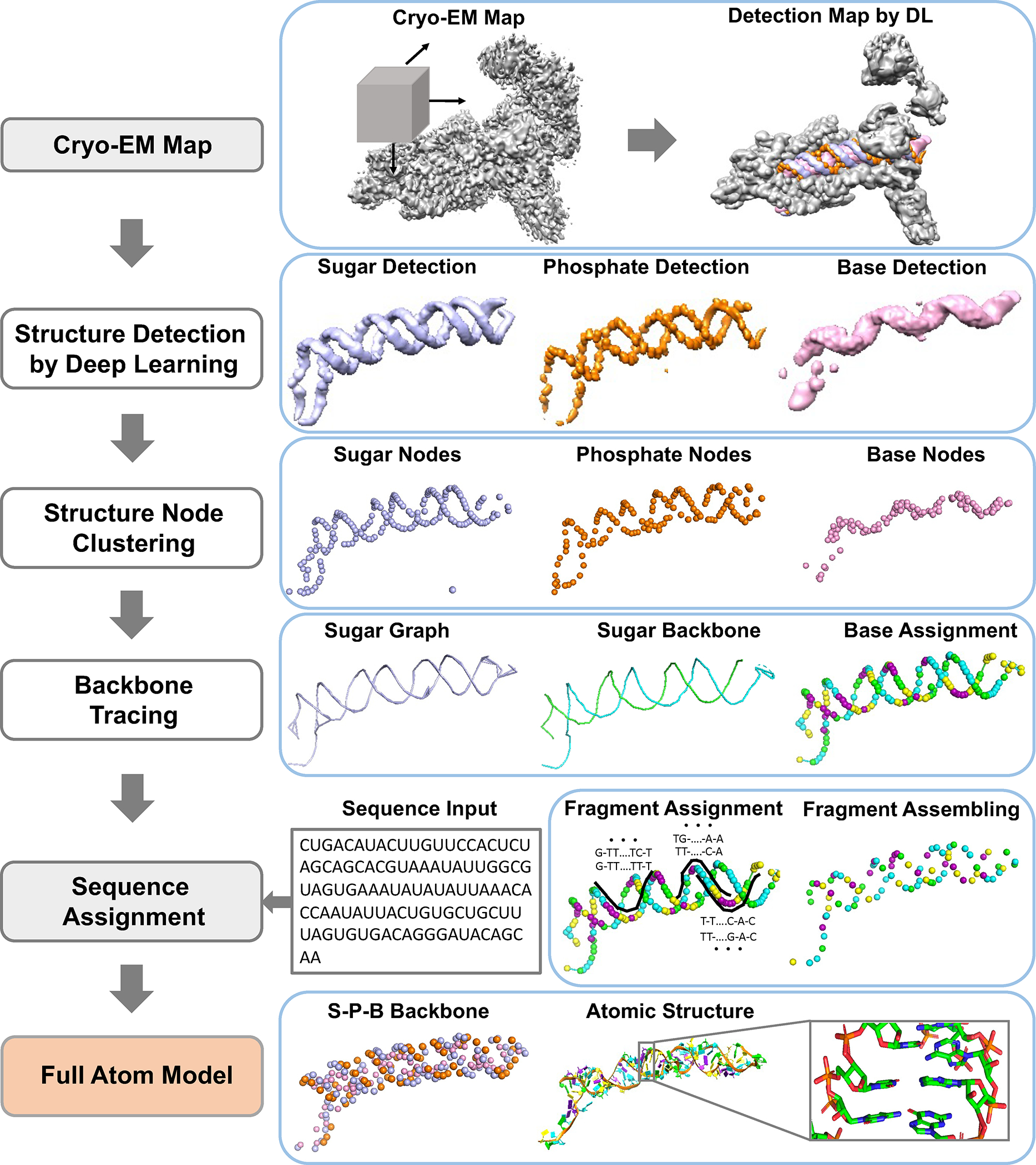
CryoREAD consists of five main steps. 1) Structure Detection by Deep Learning: locations of phosphate, sugar, base, and four base types are detected by two-stage networks. 2) Structure Node Clustering: representative nodes are identified through clustering from detected grid positions. 3) Backbone Tracing: the backbone is traced by the graph constructed with representative sugar nodes. 4) Sequence Assignment: Sequences are assigned to local fragments along the backbone path, which are then assembled in the subsequent step. 5) Full Atom Model: full nucleotides are constructed according to triangles of phosphate, sugar, and base (S-P-B) node followed by atomic structure refinement. For more details, see Methods.
Structure Detection by Deep Neural Network.
To start the structure modeling procedure, the probability of phosphate, sugar, and base at each grid position of an input density map is computed by a deep neural network. The input map is scanned with a 643 Å3 box with a stride of 16 Å along the map grid of an interval of 1 Å. The box takes density values at each grid point in the box as input features and outputs the probabilities that heavy atoms of protein, sugar, phosphate, and base for each grid point. The network architecture consists of two networks, stage 1 and stage 2, where the stage 2 network further refines the initial stage 1 output by considering the probabilities assigned by the stage 1 network. For the stage 1 network, we designed a cascaded two stage U-Net architecture 18,19 with deep supervision. We provided the network architecture in Extended Data 1.
Backbone Structure Tracing.
The next logical step is tracing the backbone of the nucleic acid from the structure classes detected by the deep neural network. It consists of two sub-steps: clustering grid points with detected structure classes to choose representative nodes and connecting representative nodes classified as sugar to construct backbone structure candidates. The clustering aims to reduce the number of grid points and to identify representative points for a structure class. Clustering was applied for all but protein class (i.e. seven classes in total; sugar, phosphate, base, and four bases, which are A, C, G, U/T). For sugar and phosphate, we selected grid points with a predicted probability of 0.1 or higher. For (general) base and base types, a probability cutoff of 0.25 was used to prescreen grid points. Then, we applied mean-shifting algorithm 10,20 to the selected representative grid points, which identifies a reduced number of local points that have relatively high predicted probability and can thus be assumed representative of their local regions.
Then, the representative nodes of the sugar prediction are connected into a graph. Only sugar nodes were used to trace the backbone since the detection accuracy for sugar was higher than phosphate and considering sugar was sufficient for tracing. Edges are connected between sugar nodes depending on the sugar probability of the nodes and the distance between them. Then, we traced the backbones of nucleic acids with a Vehicle Routing Problem (VRP) solver 21. The VRP is similar to the Traveling Salesman Problem (TSP), but it uses multiple “vehicles” instead of a single “salesman” to connect edges in a graph while minimizing connecting costs. We found VRP is more suitable since a map may include multiple nucleic acid chains. For more technical details see Methods.
Sequence Assignment to Sugar Backbone Paths.
The third step is to assign nucleic acid sequences to sugar nodes in the paths. This process has two sub-steps, first to assign base sequence fragments to paths, then to assemble assigned sequences. In the initial base sequence assignment, sugar backbone paths are cut into segments of 20 representative nodes by a sliding window with a stride of 2, which are aligned with the nucleic acid sequence to identify the top 20 candidate sequence fragments using a dynamic programming algorithm. Subsequently, the assigned sequence fragments are assembled by a constraint programming (CP) 22 solver, which maximizes the sum of the probability score of sugar nodes with the assigned bases while satisfying constraints that are required for consistency of overlapping path segments and nucleic acid sequences.
DNA/RNA Atomic Structure Modeling.
Up to this step, the structure consists of the sugar backbone and bases that are assigned to representative sugar nodes. Then, to the sugar nodes, phosphate and base nodes that are in close proximity and satisfy a distance condition are added to the model (see Methods). Next, a full-atom nucleotide 3D structure of the standard conformation is superimposed to each triangle of sugar, phosphate, and base nodes. Finally, the structure is further refined by applying phenix.real_space_refine 23 on predicted RNA regions followed by all_atom_refine in Coot 13. This is a fully automated process.
Computational Time.
We provided computational time of each step of CryoREAD for 11 maps of different sizes. Depending on the size of the nucleotides in the map, it took about 0.25 (for a small RNA of 72 nt.) to 11 hours (over 4000 nt.) to process by CryoREAD. Details are in Extended Data 2.
Structure Modeling Performance Evaluation
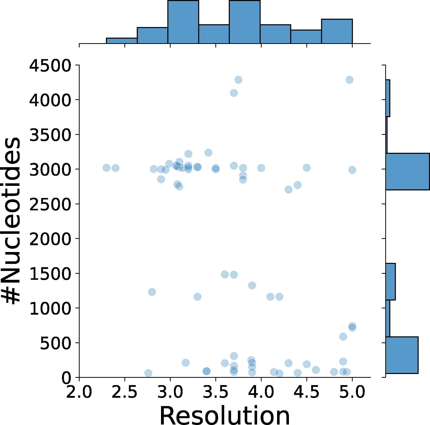
We evaluated the performance of CryoREAD on an independent dataset of 68 maps determined at resolutions between 2.0 Å and 5.0 Å. These structures are not redundant with the training and validation data we used (see Methods). The list of maps in the dataset is provided in Supplementary Table 1_Testing. The number of nucleotides included in the maps ranged from 57 to 4,286, and the number of DNA/RNA chains ranged from 1 to 6 (Extended Data 3). The dataset covers both large RNA/DNAs that have lengths over 2,500 nucleotides as well as small ones with fewer than 200 nucleotides in maps at different resolutions.
First, we discuss the accuracy of detecting structural classes in nucleic acids by deep neural networks. Fig. 2a shows the detection performance of the structural classes by the 2-stage deep networks. A nucleotide moiety was considered as correctly detected if the majority of the atoms in the moiety were correctly detected. Performance evaluated at the grid level is provided in Extended Data 4. 90.1%, 82.9%, and 89.8% of sugar, phosphate, and base moieties, respectively were detected correctly. For base fine-grained detection, individual base types, A, U/T, C, G, were detected at 55.0%, 53.0%, 65.4%, and 80.7%, respectively. Comparing results from the stage 1 and 2 networks, a clear improvement was observed from the stage 2 network, except for detecting adenine. The improvement by the stage 2 network is consistent with our previous works 11,24, where results of neighboring boxes helped improve detection accuracy. Results for individual maps are provided in Supplementary Table 2_moiety stage 2. Supplementary Table 2_grid stage 2 also includes individual map results for grid-based accuracy as well as cluster-averaged results, where results of maps in the same clusters are averaged. In Extended Data 5, we examined nucleotide moiety accuracy relative to the map resolution. Base detection accuracy was stable to the map resolution (Extended Data 5a). Detecting purine bases, adenine and guanine, which have two rings, were less affected to the map resolution than single-ring nucleotides (Extended Data 5b, 5c). When individual base types were considered, the accuracy stayed at over 0.8 until a resolution of about 3.5 Å it and started to decrease as the resolution worsened.
Fig. 2. Performance of modeling structures of nucleic acids by CryoREAD.
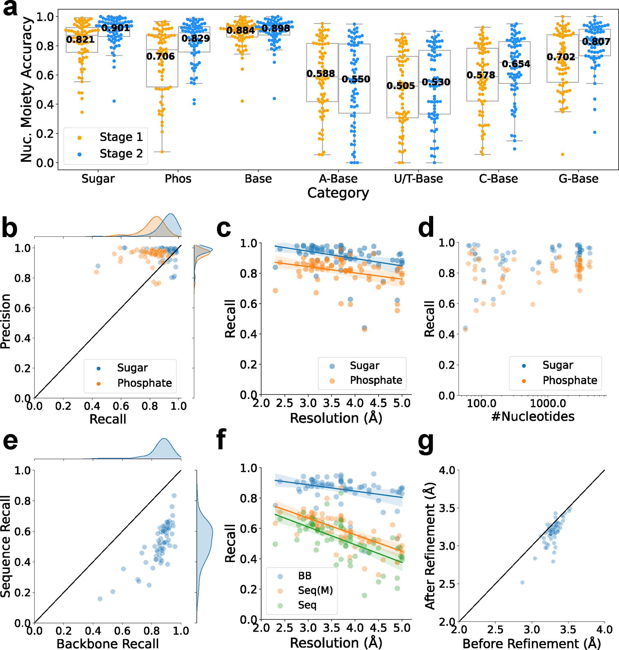
a. Nucleotide moiety-based accuracy of two stages of neural network. See Methods for the metric. The statistics are calculated over independent experimental EM maps, with each points values derived from Supplementary Table 2_ moiety stage 2. For stage 1, the values of minima, maxima, center, bounds of box and whiskers of different categories in order: Sugar(0.345,0.991,0.872,0.754/0.925,0.554/0.991), Phos(0.075,0.966,0.772,0.517/0.875,0.075/0.966), Base(0.421,1.000,0.910,0.859/0.937,0.742/1.000), A-Base(0.055,0.953,0.588,0.417/0.815,0.055/0.953), U/T-Base(0.000,0.880,0.524,0.307/0.728,0.000/0.880), C-Base(0.057,0.927,0.588,0.422/0.782,0.057/0.927), G-Base(0.057,1.000,0.718,0.550/0.876,0.348/1.000). For stage 2, the values of minima, maxima, center, bounds of box and whiskers of different categories in order: Sugar(0.421,1.000,0.929,0.864/0.964,0.734/1.000), Phos(0.404,0.988,0.889,0.757/0.931,0.541/0.988), Base(0.439,1.000,0.918,0.874/0.952,0.771/1.000), A-Base(0.000,0.948,0.571,0.339/0.812,0.000/0.948), U/T-Base(0.000,0.899,0.552,0.333/0.769,0.000/0.899), C-Base(0.094,0.950,0.685,0.541/0.827,0.150/0.950), G-Base(0.208,1.000,0.833,0.731/0.912,0.542/1.000). b. Recall and precision of sugar and phosphate atoms. c. Recall of detecting sugar and phosphate atoms relative to the map resolution. Linear regression lines are shown. For sugar atoms, the equation of regression line is (Pearson correlation coefficient: −0.361, p-value: 0.002, standard error:0.015). For phosphate atoms, the equation of regression line is (Pearson correlation coefficient: −0.301, p-value: 0.013, standard error:0.016) d. Recall of detecting sugar and phosphate atoms relative to the length of nucleic acids (on a logarithmic scale). e. Sequence assignment recall relative to the backbone recall. Sequence recall considers the fraction of nucleotides in the reference structure that were recovered by the model (see Methods). f. Backbone recall (BB), sequence recall (Seq), and sequence match (Seq (M)) relative to the map resolution. Sequence match only considers nucleotides in the reference structure that have a corresponding nucleotide in the model (an average atom pair distance of less than 5 Å). For BB, the equation of regression line is (Pearson correlation coefficient: −0.320, p-value: 0.008, standard error:0.015). For Seq, the equation of regression line is (Pearson correlation coefficient: −0.632, p-value: 7.280e-9, standard error:0.018). For Seq(M), the equation of regression line is (Pearson correlation coefficient: −0.684, p-value: 1.231e-10, standard error:0.014). The correlation between sequence recall and sequence recall (match) is provided in Extended Data 6. g. Backbone RMSD of models before and after the structure refinement. Supplementary Table 3 for details of the structure modeling performance of each map.
Next, we examine the backbone level accuracy of constructed structure models in the subsequent panels, Fig. 2b to 2g. We computed recall and precision of sugar and phosphate nodes in the Sugar-Phosphate-Base (S-P-B) conformation that were used to build the atomic detailed structure (Fig. 1, the last step). The recall of sugar and phosphate basically reports the fraction of sugar and phosphate moieties in the nucleic acids in the map that were modelled correctly (see Methods), while the precision of sugar and phosphate reports the fraction of correctly modeled moieties in a modelled structure (Methods). In Fig. 2b, sugar and phosphate moieties were detected at high recall, 0.910 and 0.814, respectively. The precision values were comparable to the recall values (Fig. 2b). Sugars were detected with a higher recall than phosphate, which was the reason that we used sugar nodes to trace the backbone in the initial step. The recall of all sugar and phosphate atoms, which we later call the backbone-level recall, was 0.857. As shown in Fig. 2c, detection did not deteriorate sharply with lower map resolutions. Also, the detection did not depend on the number of nucleic acids in the maps (Fig. 2d).
We further evaluated base sequence assignment accuracy in Fig. 2e and 2f. In Fig. 2e we show how the base recall correlates with the backbone recall. The average base recall is 0.525. It has an apparent correlation with backbone recall when examined for individual maps. For maps that have higher than 0.8 backbone recall, the average base recall is 0.556. Fig. 2f shows the base assignment performance relative to the map resolution. The base recall has a slightly stronger dependence on the resolution than the backbone atom assignment. At a resolution around 3 Å, the sequence recall is about 0.6, which went down to about 0.5 for maps at a resolution around 5 Å. We show two values for sequence recall, one that considers all the nucleotides in the nucleic acid sequences in the map and the other which only considers nucleotides in the reference structure that have a corresponding nucleotide in the model with an average atom pair distance of less than 5 Å. On average, the sequence recall (match) is higher by 0.06 than the sequence recall (Extended Data 6). In Extended Data 7, we further show the sequence matching accuracy of individual bases. Compared to nucleotide moiety accuracy shown in Extended Data 5, sequence matching accuracy has less dependency to the map resolution because sequence alignment often can fix incorrectly detected base types.
The last step in the modeling procedure is structure refinement. The refinement is aimed at correcting stereochemistry of the structure model, including removing atom clashes (defined as non-bonded atom pairs closer than 3.0 Å), placing covalently bonded atoms at a proper distance, and helps to make regular base pairs. The reduction of atom clashes is evident in Extended Data 8. Consequently, we observed improvement of RMSD to the native structure (the structure in PDB) in Fig. 2g. The average improvement of RMSD was 0.10 Å (from 3.29 Å to 3.19 Å). The largest improvement observed was from 3.29 Å to 2.79 Å. RMSD between the center of predicted bases and the corresponding native bases in matched regions (base RMSD) was 3.10 Å (Supplementary Table 3_with sequence after refine).
Fig. 3 showcases examples of nucleic acid structure models built by CryoREAD, where “DNA/RNA structure” is the native structure manually built by the authors of the cited paper, “Structure model by CryoREAD” refers to the structure automatically built by CryoREAD. The highly accurate detection by deep learning in CryoREAD provide strong foundations for further structure modeling. The first example (Fig. 3a) is the DNA-protein complex structure of hairpin-forming complex (HFC) (EMD-7480) 25, which includes six DNA chains totaling 212 nucleotides (nt) and forms a DNA hairpin structure by rotating and deforming coding-flank DNAs. The model generated by CryoREAD captured the overall topology of the DNA chains well, notably including the interaction sites of proteins and DNA, which are crucial for the function of this complex. The backbone recall was 0.862 for this model. Fig. 3b is an example of a complex with 14 proteins and a relatively small RNA of 63 nt (EMD-4868) from poxvirus RNA polymerase complexes 26. Despite the small density of the RNA, CryoREAD was able to detect the location of RNA accurately and model it. The backbone recall was 0.905.
Fig. 3. Examples of modeled atomic structure by CryoREAD for experimental maps from our testing set.
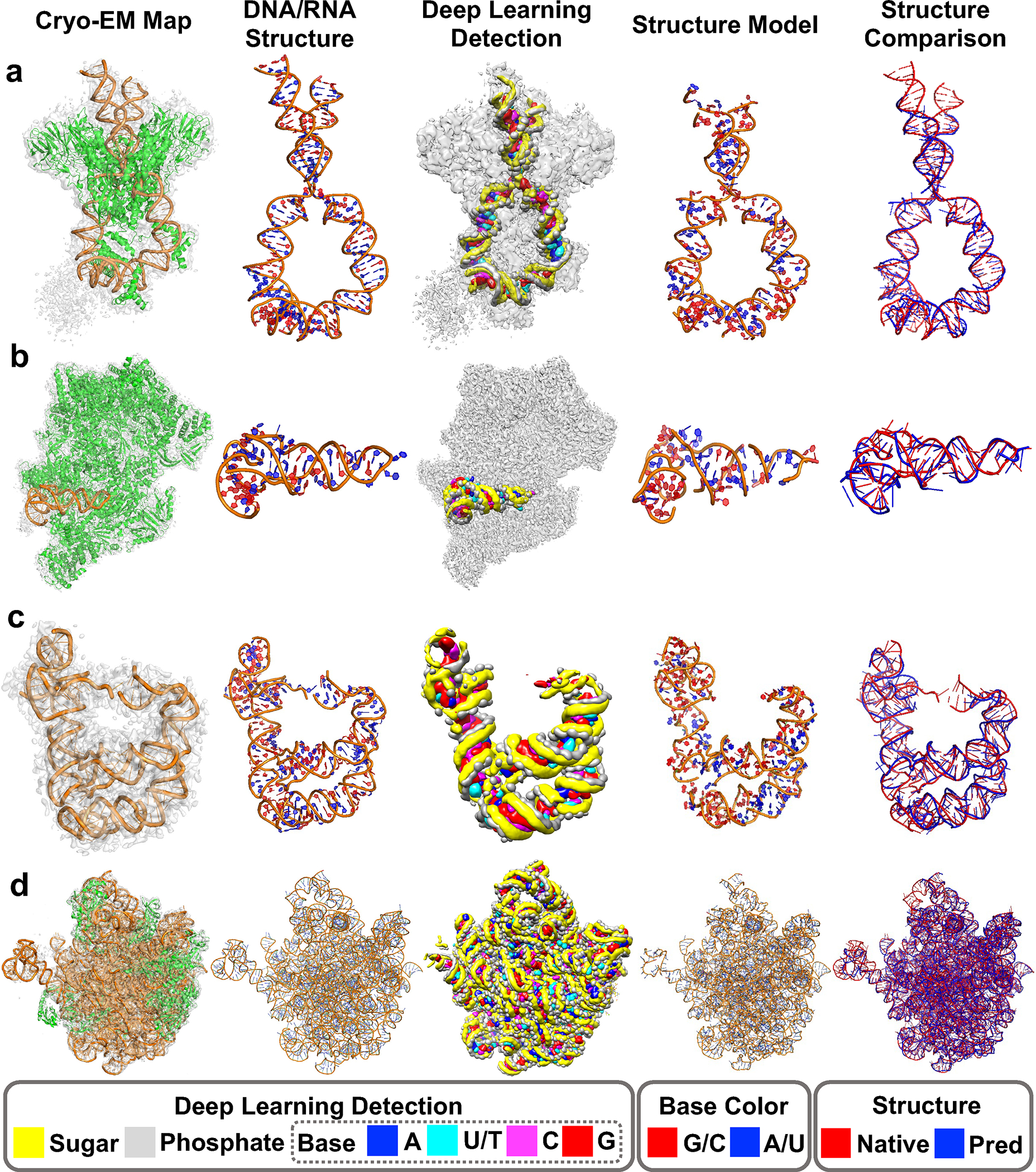
Detailed Evaluation Results are shown in Supplementary Table 3_with sequence after refine. In each row of the modeling example, five columns shown from left to right are 1) EM map and its corresponding structure; 2) only DNA/RNA structures of the native structure built by the authors of the EMDB map entry; 3) detection by deep learning network of CryoREAD. The colors indicating sugar, phosphate, and colors of bases are shown at the bottom of the figure; 4) the atomic structure model by CryoREAD. Bases are colored in red G/C and blue A/U/T. 5) Superimposition of the model (blue) with the native structure (red). a. mouse RAG1/2 HFC complex containing partial HMGB1 linker (EMD-7480, PDB-ID:6CIJ, Resolution: 3.9 Å; protein lengths: 2045 amino acids (aa); DNA length: 212 nucleotides (nt)): Backbone Recall: 0.862; Sequence Match: 0.636; Sequence Recall: 0.552; RMSD to the native: 2.83 Å. b. the complete Vaccinia DNA-dependent RNA polymerase complex (EMD-4868, PDB-ID:6RFL, Res: 2.76 Å; protein: 6191 aa; RNA: 63 nt): Backbone Recall: 0.905; Seq Match: 0.560; Seq Recall: 0.524; RMSD: 3.09 Å. c. the full-length Bacillus subtilis glyQS T-box riboswitch in complex with tRNA-Gly (EMD-20416, PDB-ID: 6POM, Res: 4.9 Å; RNA: 230 nt): Backbone Recall: 0.841; Seq Match: 0.530; Seq Recall: 0.465; RMSD: 3.26 Å. d. in vitro reconstituted 50S-ObgE-GMPPNP-RsfS particle (EMD-12217, PDB-ID:7BL4, Res: 2.4 Å, protein: 3702 aa; RNA: 3016 nt): Backbone Recall: 0.910; Seq Match: 0.706; Seq Recall: 0.661; RMSD: 3.15 Å.
In Fig. 3c, we show a map where RNA is the only determined macromolecule, a glyQS t-box-tRNAGly complex (EMD-20416), which includes 230 nt 27. This map is challenging for modeling since the resolution is low, 4.9 Å. CryoREAD detected backbone conformations well (the third panel from the left), but the atom structure model had several disconnections (the right panel). On the other hand, the backbone recall was maintained at 0.841. The last example (Fig. 3d) is a bacterial pre-50S ribosomal precursor complexed with ribosomal silencing factor RsfS and GTPase ObgE/CgtA 28. This large complex includes 3702 aa and 3016 nt, and the map (EMD-12217) is determined at 2.4 Å resolution. Despite the large size, CryoREAD was able to separate RNAs from proteins, resulting in a full atom model with a high backbone recall of 0.910. As shown in the Fig. 3d, the detected sugars and phosphates traced the backbone structures of RNAs well.
In Extended Data 9, we provide modeling results of six EM maps of ribosomal subunits. In all these six cases, CryoREAD produced RNA structure models from the entire map, while the authors of the EMDB entries have built structure models for only local density regions that were most relevant to their biological discussion. Evaluation of our models was performed only for RNAs that have associated structures and included in the provided statistics. Backbone recall of RNAs with the reference structure built by the authors of the entries ranged from 0.856 to 0.914. Additionally, we also evaluated our RNA models in unfilled density regions by comparing against relevant structures built for different maps found in PDB by sequence similarity search. There, the backbone recall values were between 0.784 and 0.847, which were similarly high as the overall benchmark results.
Modeling of SARS-CoV-2-related structures
We further applied CryoREAD to 61 EM maps of SARS-CoV-2 related structures (see Methods). The list of maps is shown in Supplementary Table 4. The structures in the maps include RNAs and proteins that are involved in translation, replication, maintaining the structure, and drug interactions of SARS-CoV-2. We applied CryoREAD as it is, using the same trained model as were trained in the benchmark study discussed above. Thus, no new training was performed for the SARS-CoV-2 map dataset. All but 3 among 61 maps have associated atomic structures in PDB. The number of nucleotides in these maps ranged from 19 to 5,982, and the number of RNA chains ranged from 1 to 7.
In Fig. 4a, we examined the modeling performance of CryoREAD on 58 maps that have associated atomic structures. The average backbone recall was 0.818 with sequence match of 0.649, and sequence recall of 0.544, which are consistent with the benchmark dataset discussed in Fig. 2. The recall values depended on the map resolution similar to what we observed in the benchmark dataset (Fig. 2f). The results of individual maps are provided in Supplementary Table 5_with sequence after refine.
Fig. 4. Atomic structure modeling by CryoREAD for experimental maps from SARS-Cov-2 benchmark.
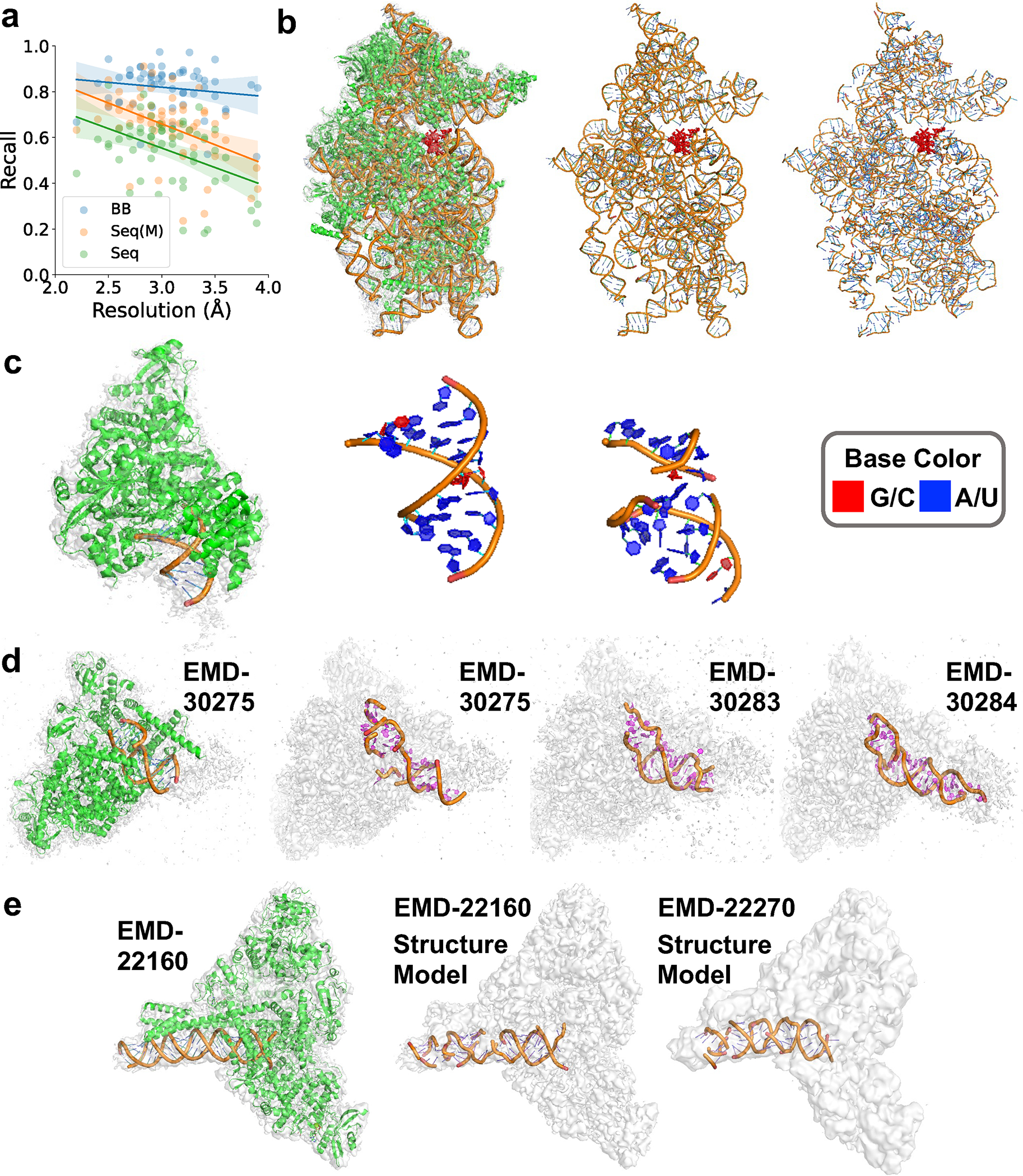
a. the backbone recall (BB), sequence recall (Seq), and sequence match (Seq (M)) relative to the map resolution. Modeling results for the 58 maps that have associated structures were used. For BB, the equation of regression line is (Pearson correlation coefficient: −0.157, p-value: 0.239, standard error:0.035). For Seq, the equation of regression line is (Pearson correlation coefficient: −0.425, p-value: 0.001, standard error:0.048). For Seq(M), the equation of regression line is (Pearson correlation coefficient: −0.460, p-value: 2.844e-4, standard error:0.047). The results of individual maps are provided in Supplementary Table 5_with sequence after refine. b. SARS-CoV-2-Nsp1-40S complex (EMD-11320, PDB ID: 6ZOJ). Resolution: 2.8 Å; protein lengths: 4914 aa; RNA length: 1704 nt: Backbone recall: 0.909; Sequence match: 0.678; Sequence recall: 0.640. From left to right, the EM map and the corresponding structure; only RNA structure in the PDB entry; the atomic structure model by CryoREAD. NSP1 of SARS-CoV-2 is shown in red. c. Nsp7-Nsp8-Nsp12 SARS-CoV2 RNA-dependent RNA polymerase in complex with template:primer dsRNA and favipiravir-RTP (EMD-11692, PDB ID: 7AAP). Resolution: 2.5 Å; protein lengths: 1120 aa; RNA length: 21 nt. Backbone recall: 0.773; Sequence match: 0.75; Sequence recall: 0.571. d. COVID-19 RNA-dependent RNA polymerase pre-translocated catalytic complex (EMD-30275, PDB-ID:7C2K). Resolution: 2.93 Å; protein lengths: 1256 aa; RNA length: 31 nt. Backbone recall: 0.831; Sequence match: 0.630; Sequence recall: 0.548. We built models for maps in two independent conformations, the conformation I (EMD-30283, Resolution: 3.03 Å) and the conformation II (EMD-30284, Resolution: 3.12 Å). We used COOT to refine the structure models by CryoREAD. e. SARS-CoV-2 replication-transcription complex bound to nsp13 helicase - nsp13(2)-RTC (EMD-22160, PDB ID: 6XEZ). Resolution: 3.5 Å; protein lengths: 2563 aa; RNA length: 70 nt. Backbone recall: 0.844; Sequence match: 0.613; Sequence recall: 0.543. On the right is the RNA model by CryoREAD for SARS-CoV-2 replication/transcription complex bound to nsp13 helicase - nsp13(1)-RTC (EMD-22270, Resolution: 4.0 Å). No structure model was associated with this map.
In the subsequent four panels, we presented examples of atomic structure models by CryoREAD. The first example (Fig. 4b) is CoV-2-Nsp1-40S complex (EMD-11320, resolution: 2.8 Å), which includes 1704 nt-long 18S ribosomal RNA. This structure has been solved by multiple groups 29–31 to understand the mechanism of how the host innate immune function is depressed because of the inhibition of translation by non-structural protein 1 (Nsp1) of SARS-CoV-2. Despite the large size, the RNA structure is well modelled with a backbone recall of 0.909. Particularly, the interaction site with Nsp1(within 10 Å) was modelled with a high backbone recall of 0.913.
The next example (Fig. 4c) is Nsp7-Nsp8-Nsp12 SARS-CoV2 RNA-dependent RNA polymerase (RdRp) in complex with template:primer dsRNA and favipiravir-RTP (EMD-11692, res. 2.5 Å) 32. The 21 nt-long template:primer RNA duplex in this complex helps to explain the binding mode of favipiravir-RTP at the catalytic site of RdRp. The CryoREAD model (the right panel) was able to identify and trace the double strand RNA, although the model had some missing nucleotides. The backbone recall was 0.773.
Fig. 4d is an interesting case where the authors of the entry provided three density maps of the same macromolecules, COVID-19 RNA-dependent RNA polymerase pre-translocated catalytic complex (EMD-30275, EMD-30283, EMD-30284, res. 2.93 Å, 3.03 Å, 3.12 Å, respectively) 33. The authors discussed that they observed two conformations existed for this complex and determined the complex structure from a map of mixed conformations (EMD-30275, PDB ID: 7C2K). For this map, the atomic structure model by CryoREAD had a backbone recall of 0.831. Although the authors did not build structure models for maps of two individual conformations (EMD-30283 and EMD-30284), we went ahead and modeled the structures by CryoREAD followed by structure refinement with COOT 13. Comparing the two RNA structures from the two maps, we observed the model for the conformation I (the model from EMD-30283, the middle panel in Fig. 4d) has fragmented RNA in one strand, because it is likely to be in a transition state where RNA is being polymerized, which is in a good agreement with the authors’ discussion in the paper 33. On the other hand, our model for conformation II (EMD-30284, the right panel), the state after the elongation has progressed, has a longer RNA by six nucleotides, which also agrees with what the authors speculated.
The last example, Fig. 4e, is SARS-CoV-2 nsp132-RTC (EMD-22160, resolution: 3.5 Å) and SARS-CoV-2 nsp131-RTC (EMD-22270, resolution 4.0 Å) 34. The authors of the entries only built the atomic structure from EMD-22160, which has a higher resolution (3.5 Å). The conformation of nsp13 in the two maps has some difference, but RNA structures are expected to be the same. We used CryoREAD to build models from the two maps. Our model for EMD-22160 had a backbone recall of 0.844 when compared to the structure deposited by the authors (6XEZ). CryoREAD was also able to build a model from the 4.0 Å map (EMD-22270), which resulted essentially the same structure with proper base pairing. When compared our model from EMD-22270 with the authors’ structure (6XEZ) by fitting into EMD-22270, the backbone recall was 0.751.
Comparison with Existing Modeling Methods
We compared the modeling performance of CryoREAD with the map_to_model in Phenix 35. This tool is mainly for protein structures and not specifically designed for nucleic acid structures, but we used Phenix as a reference since it is a popularly used tool and there are no de novo structure modeling methods specific for DNA/RNA to the best of our knowledge. Thus, the purpose of this comparison is solely to characterize CryoREAD but not for rigorous competitive evaluation.
In Fig. 5, we show the backbone recall and the sequence recall of CryoREAD and Phenix. For Phenix, we provided two models, those which were built from input of the entire map (orange), which was the same input as CryoREAD, and models for local regions of the maps after predicted non-DNA/RNA regions were masked out (blue, Phenix (Mask)). We ran Phenix masked because it was often observed that Phenix built fragmented structure models (i.e. small structure coverage Extended Data 10a) in the entire map including non-DNA/RNA regions. Thus, in general, Phenix models built from masked maps were more accurate than from maps without masks (Extended Data 10b). CryoREAD showed higher values than Phenix for both backbone recall (Fig. 5a) and sequence recall (Fig. 5b). The average backbone recalls of CryoREAD, Phenix (Mask), and Phenix were 0.857, 0.536, and 0.438, respectively. The average sequence recalls of CryoREAD, Phenix (Mask), and Phenix were 0.525, 0.208, and 0.174, respectively. Recall values relative to the map resolution are shown in Extended Data 10c and 10d. Phenix models results of individual maps are provided in Supplementary Table 6 (“with mask” tab for Phenix(Mask), “without mask” tab for Phenix).
Fig. 5. Comparison with models by Phenix.
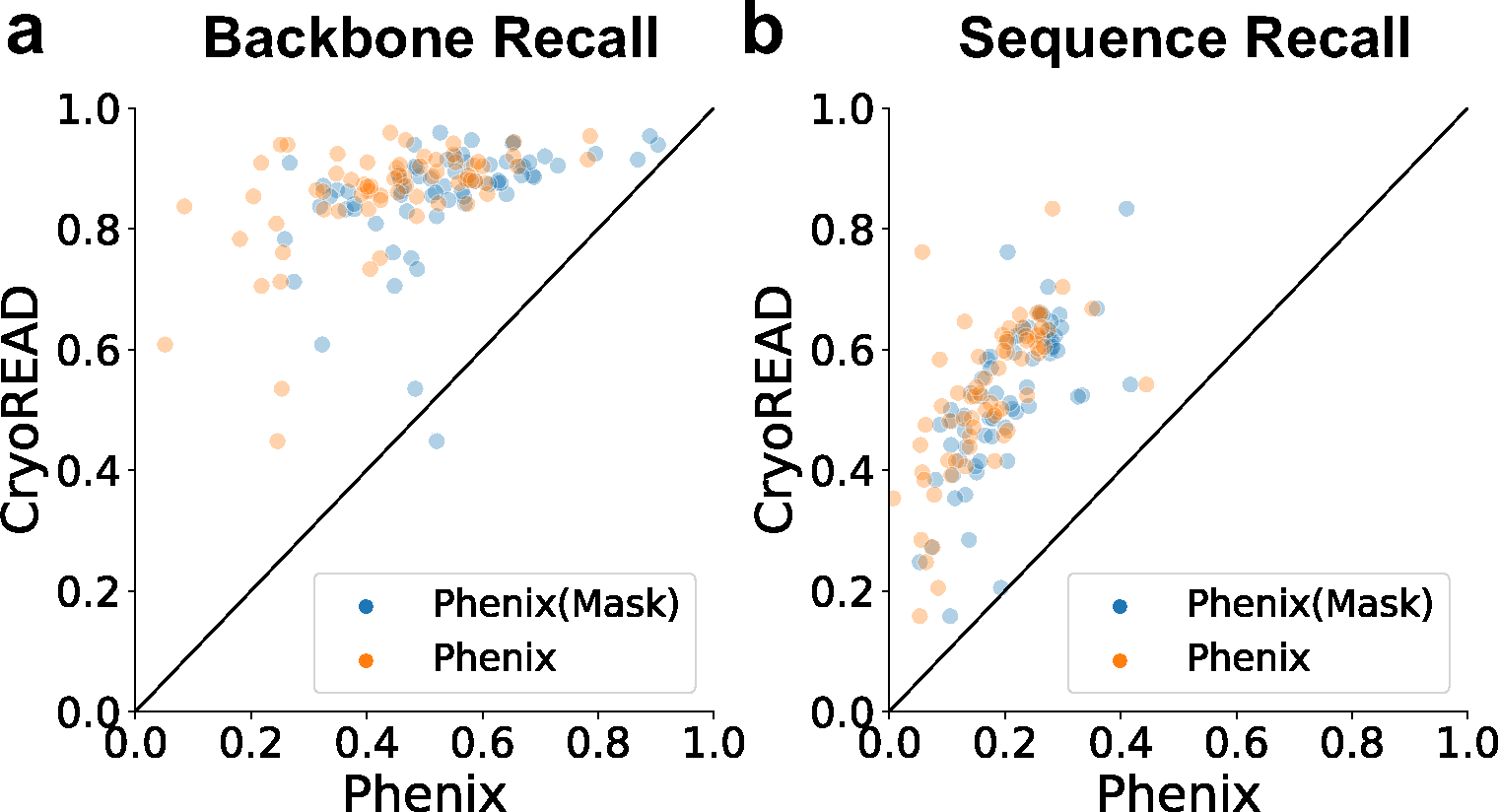
We ran the Phenix map_to_model tool in two settings. The default setting is to provide the same EM maps as input as CryoREAD (orange data points, Phenix). We also provided segmented regions of the map, which are voxels that are predicted to include nucleotides, i.e. sugar, phosphate, or bases (blue data points, Phenix (Mask)). The benchmark dataset with 68 maps were used for these plots. a, backbone recall. b, sequence recall. Other comparison data are provided in Extended Data 10 and Supplementary Table 6.
We also compared CryoREAD with auto-DRRAFTER 17. Note that auto-DDRAFTER has a different assumption and setting: It is a part of an integrated experimental and computational RNA structure modeling pipeline and thus users need to specify the location of RNA in the map if the map contains proteins (RNA-protein complex). It also assumes that accurate secondary structure information from experiments is available. In the original manuscript of auto-DRRAFTER auto-DRRAFTER was tested on relatively short RNAs with less than about 400 nucleotides. Therefore, we selected 11 maps from our testing dataset, which have RNA of a length up to 400 nucleotides. The 11 maps included ten maps of RNA-protein complexes and one map with only RNA. auto-DRRAFTER was ran in four different settings: with the map region segmented with the optimal low-pass filtering threshold to include only RNA (excluding proteins) or using a low-pass filter to include the entire map region (only small noise regions are removed); With correct or predicted secondary structure information. Detailed results are provided in Supplementary Table 7_RNA. Out of 11 maps, seven maps were not processed by auto-DDRAFTER by any low-pass filter threshold values we tried because it was not able to assign RNA helical structures into the map with confidence. The rest of the four maps included three maps with a RNA-protein complex and one with only RNA. Even when the local map region of RNA (Supplementary Fig. 1) and correct secondary structure information were provided, the average backbone recall and sequence recall were 0.509 and 0.218, respectively, which were lower than results of CryoREAD, 0.910 and 0.580, respectively. We also ran auto-DRRAFTER on ten maps that include DNA of less than 400 nucleotides from our testing dataset (see Supplementary Table 7_DNA). We provided the local map region of DNA excluding proteins and ground truth secondary structure information. Out of ten maps, four maps were not processed by auto-DRRAFTER. The average backbone and sequence recall for the rest of six maps by auto-DRRAFTER were 0.135 and 0.053, respectively, while CryoREAD had 0.827 and 0.391, respectively.
Discussion
We have developed CryoREAD, a deep learning-based method for de novo DNA/RNA atomic structure modeling for cryo-EM maps. At the target resolution range of CryoREAD, which is 2 Å to 5 Å, it is often difficult to model nucleic acid structures by conventional tools. But key structure elements of nucleic acids, phosphates, sugars, and bases can be detected by deep learning, which greatly enhances modeling capability. Deep learning is particularly accurate in separating proteins and nucleic acids in an EM map as was also demonstrated in our earlier work, Emap2sec+ 24. The modeling process is fully automated, and no human intervention is needed. We believe resulting structure model will serve as an excellent starting point for biologists to apply structure refinement and manual detailed modeling as we showed in the RNA structure modeling for SARS-CoV-2 (Fig. 4).
Although CryoREAD was shown to work well overall, it would be appropriate to discuss limitations observed in the current version. Relative to the backbone accuracy, the assignment of nucleotide sequence has room for improvement. As shown in Fig. 2a, deep learning identifies base positions with high accuracy; however, base type detection is less accurate. At relatively low resolution, distinguishing base types becomes more difficult and affects the sequence matching accuracy. However, CryoREAD provides accurate nucleic acid structures even for maps at lower resolutions and base assignment in the model will be a good starting point for manual sequence assignment. Also, we observed that the final structure model often has gaps in the backbone and incorrect base pairing conformations specially for large structures that are generally difficult to model. For such cases, manual refinement using existing tools, such as COOT, would be effective for improvement. In general, CryoREAD is intended to quickly provide the initial starting model for building nucleic acid structures, from which users can examine and further manually refine. Currently, we do not use predicted secondary structure information for nucleic acids in CryoREAD since the accuracy of predictions is not high enough. However, if the accuracy of predicted secondary structure information improves in the future, we plan to integrate it into CryoREAD.
As more structures are being determined by cryo-EM, accurate and easy-to-use modeling tools would substantially facilitate the structural determination process, allowing biologists to focus more on biology rather than technical steps in modeling. We believe CryoREAD will be a useful and powerful tool for nucleic acid structure modeling, filling the area where available tools are scarce, in the era of cryo-EM structural biology.
Methods
Constructing benchmark dataset
We prepared a dataset of experimental cryo-EM maps for training, validation, and testing of CryoREAD. First, from EMDB of June 10th, 2021, we downloaded cryo-EM maps that were determined at a resolution from 2 Å to 5 Å and had the corresponding PDB entries that contain nucleic acid structures with more than 20 nucleotides. This initial set consisted of 1,384 maps. To ensure sufficient quality of structure models in the PDB entries, we required the EM map and simulated maps from the structures in the PDB entry computed for the map’s resolution had a cross-correlation of densities of 0.65 or higher 24. This step reduced the number of maps to 548.
To handle the redundancy of the maps, we clustered maps with complete linkage considering sequence identity of proteins and nucleic acids in the maps. Two maps were clustered into the same group if any protein chains from the two maps have 30% or larger sequence identity over 50% coverage or DNA/RNA chains share 80% or larger global sequence identity. This clustering procedure resulted in 108 clusters of maps.
From the 108 clusters, we randomly selected 27 clusters (68 maps) for the testing set. Then, from the remaining maps we removed ones that are similar to the testing maps using the same criteria as the previous step, which resulted in 79 clusters (290 maps). These maps were used for training and validation. We applied this additional step of eliminating similar maps because a different cluster may still contain similar maps as the clustering was done with complete linkage. Out of the 79 clusters, we randomly selected 63 clusters (238 maps) for training and validation of the stage 1 network (Extended Data 1) and 16 clusters (52 maps) for training and validation of the stage 2 network. The 290 maps in the training and validation sets included 61 maps with DNA, 156 maps with RNA, and 21 maps with both DNA and RNA. 52 maps for the stage 2 network contained 25 maps with DNA, 24 maps with RNA, and 3 DNA and RNA. The testing dataset consisted of 11 maps with DNA 55 maps with RNA, and 2 maps with both DNA and RNA. The list of entries of the datasets is available as Supplementary Table 1.
If a map had a different grid size from 1.0 Å we interpolated the grid size to 1.0 Å by trilinear interpolation of the density. The density values in a map were normalized to [0.0, 1.0] with a minimum-maximum normalization. All negative values in a map were set to 0, and 0 was used as the minimum value for normalization. We used the 98th percentile density value as the maximum value, and any density values above that were set to 1.0.
From each map, boxes of a size of 643 Å3 were collected by scanning the box across a map along three axes with a stride of 16.0 Å. We assigned each grid point in the box with a label that were taken from the closest heavy atoms of the closest residue/nucleotide located within 2.0 Å. If a grid point is close to more than two heavy atoms, the closest heavy atom was used to provide the label. If no heavy atoms were found within 2.0 Å of a grid point, the point was assigned as background. A box was discarded if less than 0.1% of the grid points have DNA/RNA atom assignment.
Constructing dataset of SARS-CoV-2
First, from the list of SARS-CoV-2 related entries in PDB (https://rcsb.org/covid19), we selected structures that were determined by cryo-EM and have a map resolution between 2 Å to 5 Å. Then, we discarded entries that have less than 10 consecutive nucleotides. This resulted in 56 cryo-EM maps. We performed the same search also in EMDataResource (https://www.emdataresource.org/) and obtained 56 maps. These two searches were conducted on August 10th, 2022. The 56 maps from EMDataResource included 3 maps that do not have associated structure models. The two sets have 51 maps in common; thus, resulted in 61 unique maps in total. Among them 58 maps with deposited structures were used to assess the accuracy of modeling. All these maps contain RNA.
CryoREAD was not newly trained specifically to this dataset. No human intervention was performed when applying CryoREAD to the maps in this dataset. The list of entries is provided in Supplementary Table 4.
Training the deep neural network of CryoREAD
CryoREAD has two networks, stage 1 and stage 2 (Extended Data 1). As mentioned in the previous section, we allocated 238 maps for training and validation of the stage 1 network. These maps were split into 80% (190 maps) and 20% (48 maps) for training and validation, respectively. The same split of 80% (41 maps) and 20% (11 maps) were applied to the 52 maps allocated for the stage 2 network. The stage 1 network takes density values in an EM map extracted in a box of 643 Å3 as input and outputs eight 643 Å3 boxes through the cascaded network (Extended Data 1a), which has a probability of having atoms of proteins, phosphate, sugar (ribose or deoxyribose), base, and four types of bases (A, C, G, U/T) at each grid point, respectively. For each batch of training, we randomly sampled 16 boxes from the 190 maps, which totaled around 63,000 and 13,000 boxes used in an epoch for training and validation, respectively.
For training the stage 2 network, we used 52 maps that do not have overlap with maps used for stage 1 training and validation. After the training of the stage 1 network is completed, we input each of the 52 maps to the stage 1 network and obtained the output of probability values for each grid point of each map. Then, the output probability values were used as input for the stage 2 network. The size of the input box for the stage 2 network is the same, 643 Å3. The stage 2 network has a UNet++ architecture 18,19, which outputs the probability of eight structural classes. The batch size was 32 and the total number of training and validation boxes for the stage 2 network was around 8,000 and 2,000, respectively. Both stage 1 and 2 networks were trained through 10 epochs.
We used the Dice loss 36:
| (1) |
represents the Dice loss of a predicted box and a corresponding ground truth box is the total number of grid points inside the box; is the predicted probability of the i-th grid point in the predicted box; is the binary ground truth of the i-th grid point, where 1 denotes the existence of such structure in the grid point and 0 indicates no such structures; is a smoothing factor with value of 1e-6; is the overall loss of a batch of examples with class detection; represents the dice loss of k-th example’s j-th class detection.
For the training of the stage 1 network, we tested combinations of a learning rate of [2e-5, 2e-4, 0.002, 0.02, 0.2] with a L2 regularization weight of [1e-6, 1e-5, 1e-4, 0.001, 0.01, 0.1] using the Adam optimizer 37. Among the combinations, the learning rate 2e-4 with L2 regularization parameter of 1e-5 showed the best grid-wise accuracy of 81.6% on the validation set, although the performances with different combinations were similar. We used the same hyper-parameters for training the stage 2 network.
Training and validation of the stage 1 network took about 10 days using around 80,000 data. Training and validation of the stage 2 network took about 17 hours with around 10,000 box data. The computations were performed on two paralleled NVIDIA Titan RTX 24 GB GPU connected via NVLink. The training and validation loss along epochs are shown in Supplementary Fig.2. As the validation loss is almost stable at around 9–10 epochs, we stopped the training at 10 epochs. We also extended training up to 30 epochs (Supplementary Fig.2b) but did not observe a substantial decrease of validation loss.
Computing representative nodes with mean shift algorithm
Grids with larger than 0.1 probability values for sugar, phosphate, and 0.25 for base, and four base types, A, C, G, and U/T were clustered to identify representative nodes using the mean-shift algorithm. The mean-shift algorithm 20,38 is a non-parametric clustering algorithm commonly used for image processing. We use the mean-shift algorithm because it was successfully applied in our previous work on the MAINMAST algorithm for protein structure modeling from cryo-EM 10. We assume that computed probabilities correspond well to the atom distribution of the molecular structure in the cryo-EM map. Therefore, the identified representative nodes by this clustering step are expected to locate around the center of the corresponding moiety.
Mean shift iteratively updates the locations and densities (computed probability values, in this case) of the input points. Given a grid point , the function determines the weight of nearby points for re-estimation of the mean. The point is iteratively updated following until convergence when with set to 0.001. Here the updating function is shown in Eq. (2).
| (2) |
where is the neighborhood of , a set of grid points satisfied is a Gaussian kernel function with bandwidth , as shown in Eq.(3); is the probability/density value of the grid point indicates the position of i-th neighbor grid point of .
| (3) |
where the is the bandwidth set as 3.
Meanwhile, we also update the density value of the point following Eq. (4).
| (4) |
where is the updated density/probability of , is the number of neighborhood grid points of .
For different detections, we applied the mean-shift algorithm for any grid points with a probability , where is a threshold set to 0.1 for sugar and phosphate detection, 0.25 for base detection to reduce the number of false negatives.
After the mean-shifting algorithm, we first normalized all the grid points with min-max normalization following Eq. (5).
| (5) |
where are the maximum/minimum density/probability value of the converged shifted points. Points are removed if the normalized density/probability with set as 0.05. Next, any shifted points that are closer than a threshold distance (2.0 Å) are clustered, and the grid point with the maximum density/probability is selected as the representative node of the cluster. This process is iterated until the selected representative nodes converge. The remaining points are called as representative nodes.
Constructing a sugar graph
Identified sugar nodes by the mean-shifting algorithm are connected to form a graph. Given two nodes from cluster of original grid points and from cluster , they are labeled as adjacent and connected with an edge if any pair of and are originally adjacent at their initial point position, and . An edge is removed in the following operation: Five points are sampled along the edge between and at even intervals. If the base probability of the closest grid point to any of the five points is larger than 0.5, this edge is discarded because it is highly likely that the edge connection is incorrect. For example, they may be sugars across different chains in double stranded DNA or RNA. Next, two sugar nodes, and are further connected if they satisfy a distance condition, , where was set to 10 Å and if all the evenly-sampled five points along the edge have the sugar probability of 0.1 or higher and also if none of them have a base probability over 0.5. The resulting graph is denoted as .
Backbone Tracing Using Vehicle Routing Problem Solver
The next step is to trace the backbone(s) of nucleic acids in the map from the sugar graph. We formulate this task as a Vehicle Routing Problem (VRP) 39, which is a variation of the Traveling Salesman Problem (TSP). In VRP multiple vehicles are used, rather than a single salesman, as moving agents, to visit a set of nodes. All nodes are allowed to be visited up to once by any vehicles. A VRP solver aims to maximize the number of visited nodes in the input graph while minimizing the total costs of routes by all the vehicles. As multiple vehicles are used, multiple, non-overlapping paths will be identified in the graph. We found the setting of VRP fits well with our problem where we aim for identifying the backbone of multiple nucleic acid chains in a map. We used a VRP solver in the OR-tools package (https://developers.google.com/optimization/).
We identify paths in a sugar graph , which has nodes, (), where each node denotes a sugar node. A node is either included in a path or not included in any of the paths. When a node is connected, the cost is added that reflects the length of edges to the node and the probability value assigned to the edge. On the other hand, a penalty is added if a node is not visited by any vehicles thus not included in paths. As required also in TSP, all nodes are only allowed to be visited up to once. The global objective of VRP is to minimize the following cost:
| (6) |
where is the number of vehicles to traverse the graph, which is set as floor of , i.e. the maximum integer that does not exceed is the number of edges traveled by the -th vehicle, which connects edges; indicates the cost of forming the -th edge by the -th vehicle. The edge weight used in Eq. 6 is defined as follows:
| (7) |
where is the length of edge is the minimum probability value among evenly sampled 10 points along the edge. Thus, forming an edge with two nodes at a large distance and a low probability costs more. is the maximum value of among all the edges The second condition allows a connection with two nodes that are not included in but at a higher cost with distance smaller than .
In the second term of Eq. 6, is the drop penalty cost for nodes without visits by any vehicles and thus not included in backbone paths. if is not visited by any vehicles; otherwise, is defined as
| (8) |
where is defined in Eq. 7 and . With this setting, if a node that is not included in and has is included in a path, for example, it pays a cost of according to Eq. 7. On the other hand, if it is not included in any path, it pays a drop penalty of will be charged.
An example of the backbone tracing is shown in Supplementary Fig. 3. It illustrates how the sugar graph is constructed for an EM map and the backbones are traced. The VRP solver was able to trace the backbone of two RNA molecules. Comparison of number of nodes before and after VRP process are shown in Supplementary Fig. 4. The drop ratio of nodes is within 5% for most targets.
Sequence Fragment Assignment
The path(s) constructed in the previous step were scanned with a sliding window of a length of (= 20) with a stride of (= 2), and path fragments were generated. Each of the path fragment will be aligned with each of the DNA/RNA sequences in the map. For each path fragment, possible sequence assignments are kept, where is the number of DNA/RNA sequences, and 2 comes by considering both forward and reverse directions of DNA/RNA, and is the number of top scoring alignments kept.
Given a fragment of length and a single DNA/RNA chain of length , sequence alignment was performed with a dynamic programming algorithm. Rewards for a position in an alignment is defined with a matching reward and gap penalty values that consider geometry constraints:
| (9) |
where is a 2D reward matrix; is the index of nodes in the path fragment, is the index of the DNA/RNA sequence. An open gap for DNA/RNA sequence matching is not encouraged by requiring a large penalty of Dynamic programming chooses the optimal actions among three choices: matching of and (reward of matching with a potential geometry penalty, GP1), skipping the node (with a potential geometry penalty, GP2), skipping the nucleotide (with a sequence penalty, SP). indicates the reward of matching and and are the node gap penalties considering the geometry constraint. is the node of the previous alignment before to obtain the reward of or is the sequence gap penalty considering the previous alignment.
Matching score for a path position and a sequence position j: is a reward for matching and defined as , where 100 is the weighting factor to balance the reward and the penalty, is the probability of node for the base type of , computed by the deep neural network. is a gap penalty assigned if the distance of node of the previous alignment position and node of is too close or too far, which is defined as follows:
| (10) |
where is a node gap penalty set as 10; is the distance between the k-th node and the i-th node; is the mean distance between two consecutive nucleotides in nucleic acid, which is set as 7; is the minimum distance allowed for two consecutive nodes, which is set as 4; is the maximum distance allowed for two consecutive nodes, which is set as 10.
Skipping node i: When skipping node , we consider the distance between node of previous alignment and node of to decide a gap penalty. is defined as,
| (11) |
where is the distance between the k-th node and the i-th node; share the same value as inEq. (8).
Skipping nucleotide j: When skipping a nucleotide , a sequence gap, defined as following, will be applied.
| (12) |
where is the sequence gap penalty set as 25; is the accumulative number of sequence alignment gap to obtain .
Once the dynamic programming scores, , are all computed, the top scoring sequence assignments are collected.
Sequence Fragment Assembly
Identified sequence-node fragment alignments are assembled. For each node path fragment, alignments with nucleic acid sequences are obtained. We applied constraint optimization/programming (CP) 22 to solve the assembly problem. CP aims to find feasible solutions out of a very large set of candidates with arbitrary constraints. The goal of CP is to maximize the sum of , which have been collected in the previous alignment step under two constraints, which we call the node fragment-based constraint and the sequence-based constraint. We used the cp_solver library available at https://developers.google.com/optimization/cp/cp_solver.
Node fragment-based Constraints.
The first constraint is assuring the uniqueness of the sequence alignment for a node path fragment; i.e. only one sequence assignment is selected for the same node fragment. We check the overlap of all the pairs of node fragments and apply two more constraints for overlapping pairs. Two overlapping fragments cannot be selected together if their sequence assignments are from two different directions, forward and reverse or from two different chains. Also, for an overlapping node region of two fragments, their sequence assignments must have at least 80% identity and the sequences. The sequence of higher matching score will be selected.
Sequence-based constraint.
If two alignments of a sequence fragment and a node fragment do not have overlap in node fragments but have an overlap in their sequence assignments they are not selected together because it is not physically possible to match neighboring sequence regions to different locations in a map. The two sequence regions are considered as having overlap if the overlap is longer than 20% of the assigned sequence length (the shorter of the two).
To increase the base assignment accuracy and coverage, once the CP solver outputs the assembly result, two post processing steps are applied. First, for a region in the node paths that are covered by overlapping sequence fragments, we align the assigned nucleic acid sequences against the region once again and update the sequence assignment. Next, for short regions in the node paths that are not yet covered by nucleotide sequences, which typically happen as a short sequence assignment gap between two assigned regions, we align the region with the nucleic acid sequences and assign the highest scoring sequence to fill the gap.
Building Atomic Structure
To the constructed sugar node backbone, we add the closest phosphate node for two consecutive sugar nodes if the sum of their distances is within 14 Å. The sugar-phosphate backbone is constructed from the phosphate and sugar node assignments. Next, base nodes are associated with each sugar-phosphate pair by selecting the closest base node. The three nodes of Sugar, Phosphate and Base (SPB) allow for the initial atomic nucleotide assignment. We assign the standard nucleotide structures taken from PDB to each SPB based on rigid transformation. For the rigid transformation, the phosphate node in the SPB and the phosphate center in the standard nucleotide, the normalized direction vector from the phosphate node to the sugar node in the SPB and the vector from the phosphate center to the sugar center in the nucleotide structure, and the normalized vector from the phosphate node to the base node in the SPB and the vector from the phosphate center to the base center in the nucleotide structure, are aligned. Finally, the structure is refined with phenix.real_space_refine 23 on predicted RNA regions followed by all_atom_refine in Coot 13.. The phenix command used was “phenix.real_space_refine [model structure] [EM_Map] resolution=[map_resolution]”.
Evaluation Metrics
Here we summarize the evaluation metrics used in this study.
Moiety-Level Accuracy:
A moiety was considered to be correct if the majority of atoms in the moiety is correctly detected. An atom was considered as correctly detected if the majority of the grid points closer than 2 Å to the atom have correct structure class assignment.
Recall:
Recall of sugar and phosphate was computed as the fraction of sugar atoms (C1’, C2’, O2’ for RNA, C3’, O3’, C4’, O4’, C5’) and phosphate atoms (P, OP1, OP2, O5’, OP3’) that were closer than 5 Å to a matched sugar or phosphate node for each nucleotide, which were then averaged over all the nucleotides in the map. Here matched sugar/phosphate node was with average distance within 5 Å between the node and corresponding atoms.
Backbone recall considers atoms from both sugar and phosphate.
To compute sequence recall, first we identified a nucleotide in the model that corresponds to each nucleotide in the reference structure by assigning the nucleotide in the model that has the closest average atom distance, then checked if the bases are identical or not. Then we computed the fraction of the identical bases over all the bases in the reference structure. Sequence recall match only considers nucleotides in the reference structure that have a corresponding nucleotide in the model (an average atom pair distance of less than 5 Å).
Precision:
Precision of sugar and phosphate nodes is defined as the fraction of nodes that are within 5 Å to its corresponding atoms of its closest nucleotides. 5 Å was used as the cutoff because it is shorter than the average distance between adjacent phosphate atoms, which is 6.0 Å. We only considered sugar and phosphate atoms in the model that are closer than 10 Å to any atoms in the reference structure.
Similar to sequence recall, sequence precision is defined as the fraction of the identical bases over all the bases in the model. sequence precision (match) only considers nucleotides in the model structure that have a corresponding nucleotide in the reference (an average atom pair distance of less than 5 Å).
Comparison with Phenix and Auto-Drrafter
For Phenix, we ran map_to_model in Phenix 35. For the unmasked mode running, we provided the original cryo-EM map file, the sequence file, resolution and symmetry information if it is available. For the masked mode running, we first masked protein regions of cryo-EM map by CryoREAD’s detection of proteins and provided masked cryo-EM map for Phenix to run. All other settings were the same as the unmasked mode.
For Auto-DRRAFTER17, we visually inspected the map and the corresponding deposited structure to find an optimal low-pass filtering threshold to include only RNA (excluding proteins). Then we used two different secondary structure information to run separate experiment: the ground truth secondary structure information from deposited structure and predicted secondary structure predicted by RNAFold40. As suggested in official tutorials (https://www.rosettacommons.org/docs/latest/application_documentation/rna/auto-drrafter), we provided an cryo-EM map, sequence information, secondary structure information, and the manually inspected threshold value as input to run auto-DRRAFTER with three rounds optimization to obtain a final structure.
Extended Data
Extended Data 1. The detailed network architecture of cryo-READ.
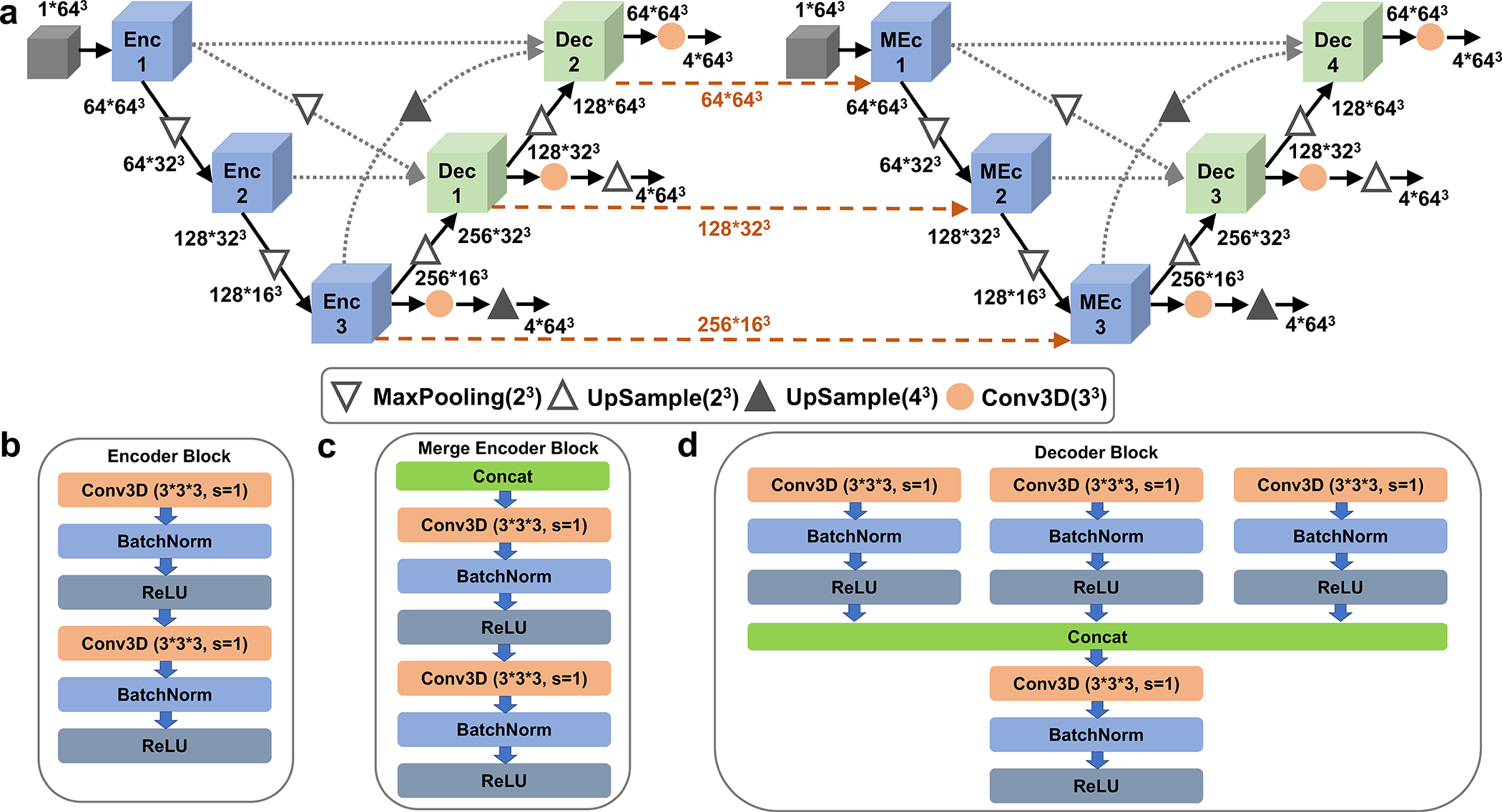
a, the network architecture. The entire network consists of two stages of U-Net networks and here we show the 1st stage networks. It concatenates two U-Net architectures. They are 3D U-shape-based convolutional Network (UNet) with full-scale skip connections and deep supervisions. The channel size of different layers is also illustrated in the figure. b, The Encoder Block (Enc1 in panel a); c, The Merge Encoder Block (MEnc); and d, the Decoder Block (Dec). Conv3D, a 3-dimentional (3D) convolutional layer with the filter size of 3*3*3, stride 1 and padding 1. BatchNorm, a normalization layer that takes statistics in a batch to normalize the input data. ReLU, Rectified Linear Unit, a commonly used activation layer.
It is a cascaded U-net, where the first U-Net (on the left) focuses on the prediction of high-level detection of sugar, phosphate, base, and protein while the second U-Net (on the right) focuses predicting different base types: A, C, G, and T/U. The processed information of the 1st U-Net encoder is also passed as input for the 2nd U-Net to help its predictions (dashed lines in orange). We applied deep supervision to the loss on output of different decoder outputs, which was shown to improve the performance. The stage 2 network only includes the first U-Net architecture of the stage 1 network. It takes predicted probabilities of 8*643 Å3 predictions (8 probabilities: protein, phosphate, sugar, base, and four different base types) from the stage 1 network and outputs the refined probabilities in a box of 8*64*64*64 Å3.
Extended Data 2. The running Time of CryoREAD on 11 structures of different sizes.
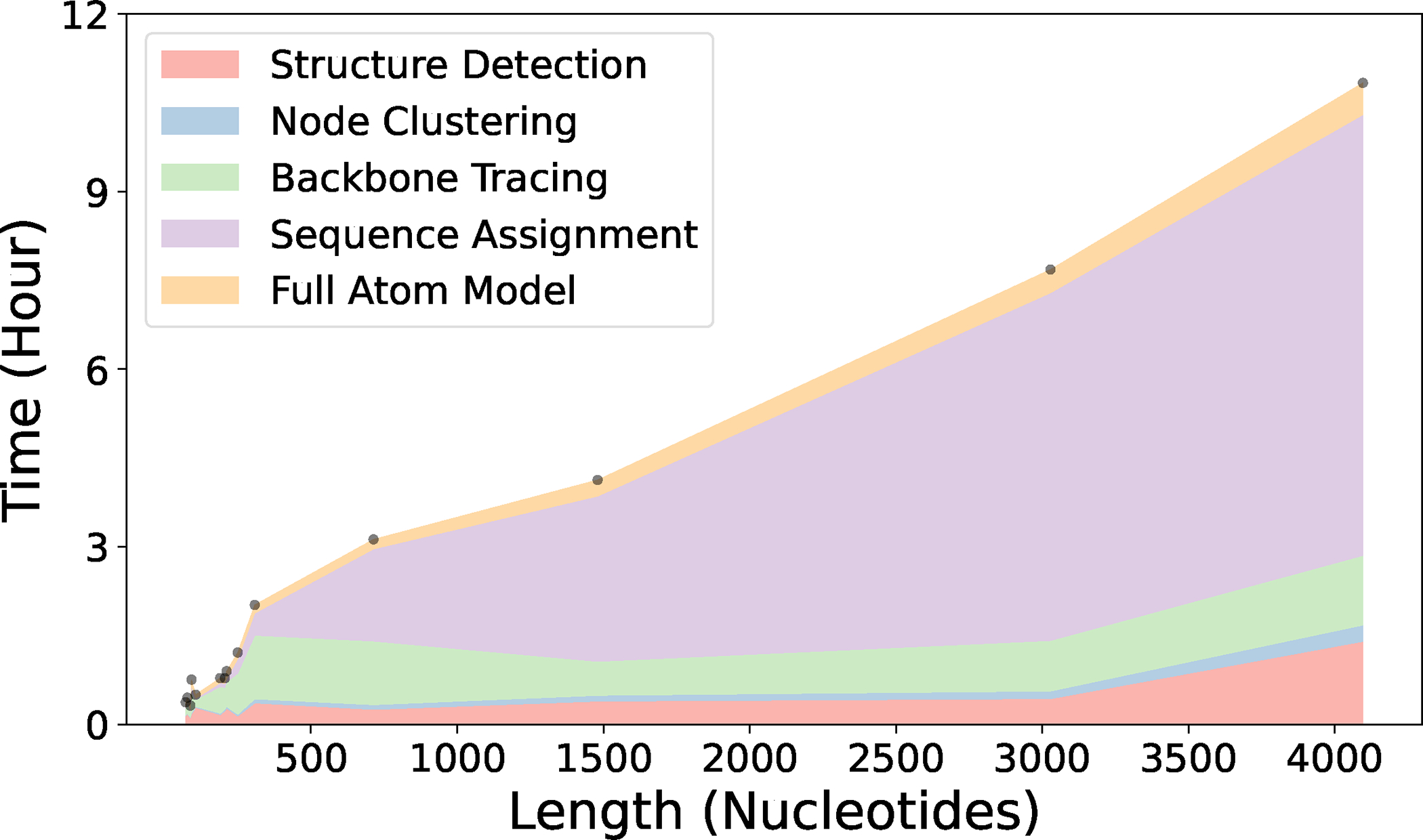
The experiments were carried out on a computer server with 1 NVIDIA TITAN RTX 24GB GPU and 24 CPUs. Here 5 colors correspond to 5 steps in CryoREAD pipeline: 1) Structure Detection by Deep Learning; 2) Representative Node Clustering; 3) Backbone Tracing; 4) Sequence Assignment; 5) Full Atom Model. The actual data point of the 11 maps are shown by dots.
Extended Data 3. The distribution of the size of nucleic acids in the 68 cryo-EM maps in the test set relative to the map resolution.
Extended Data 4. Grid level detection accuracy (recall) of 8 structural classes.

A grid was assigned with a structure class that is closer than 2 Å to the grid. If there were multiple different structures that were within 2 Å, the closer one was assigned to the grid. A detection by deep network for a grid was considered as correct if the probability of the correct structure class has a value over 0.5. pho, phosphate. Results of the stage 1 and stage 2 networks are shown. The statistics are calculated over independent experimental EM maps, with each points values derived from Supplementary Table 2. For stage 1, the values of minima, maxima, center, bounds of box and whiskers of different categories in order: Sugar(0.333,0.893,0.729,0.601/0.804,0.333/0.893), Phos(0.138,0.849,0.656,0.463/0.754,0.138/0.849), Base(0.380,0.947,0.836,0.772/0.889,0.669/0.947), Protein(0.349,0.929,0.808,0.763/0.879,0.621/0.929), A-Base(0.034,0.890,0.549,0.362/0.746,0.034/0.890), U/T-Base(0.019,0.797,0.460,0.294/0.646,0.019/0.797), C-Base(0.088,0.886,0.539,0.369/0.711,0.088/0.886), G-Base(0.153,0.933,0.637,0.490/0.823,0.153/0.933), Overall(0.438,0.909,0.764,0.685/0.822,0.478/0.909). For stage 2, the values of minima, maxima, center, bounds of box and whiskers of different categories in order: Sugar(0.357,0.920,0.775,0.654/0.846,0.453/0.920), Phos(0.228,0.883,0.693,0.509/0.810,0.228/0.883), Base(0.408,0.952,0.858,0.795/0.905,0.695/0.952), Protein(0.490,0.969,0.903,0.867/0.936,0.772/0.969), A-Base(0.013,0.893,0.501,0.296/0.745,0.013/0.893), U/T-Base(0.024,0.824,0.479,0.291/0.682,0.024/0.824), C-Base(0.104,0.920,0.611,0.449/0.775,0.104/0.920), G-Base(0.237,0.951,0.737,0.609/0.858,0.237/0.951), Overall(0.492,0.952,0.827,0.756/0.878,0.577/0.952). For the moiety level accuracy, see Fig. 2 in the main text.
Extended Data 5. Nucleotide moiety-based accuracy relative to the resolution.
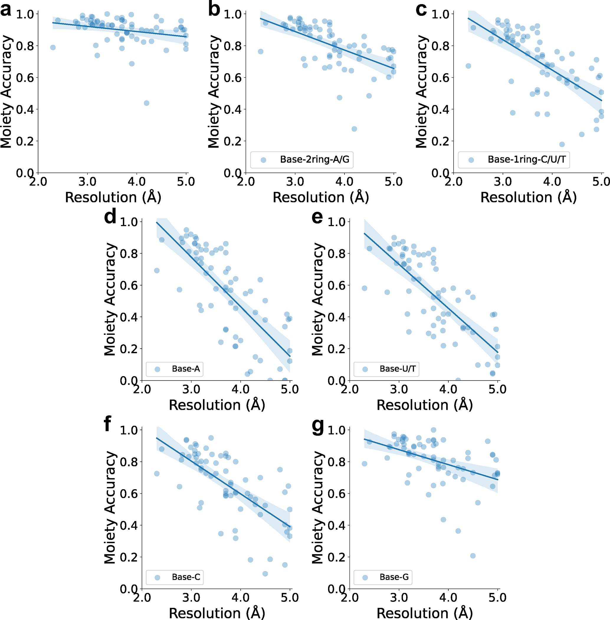
A nucleotide moiety was considered as correctly detected if the majority of the atoms in the moiety were correctly detected. The data used here is the same as those which were used for Fig. 2a. a. base detection accuracy relative to the map resolution. The equation of regression line is (Pearson correlation coefficient: −0.256, p-value: 0.035, standard error:0.015). b. Moiety-based accuracy of detecting 2-ring bases (A/G). If A or G was detected as either A or G, it was considered as correct detection. The equation of regression line is (Pearson correlation coefficient: −0.582, p-value: 1.925e-7, standard error:0.020). c. Accuracy of detecting 1-ring bases (U/T/C). The equation of regression line is (Pearson correlation coefficient: −0.658, p-value: 1.109e-9, standard error:0.027). d. Accuracy of detecting Adenine (A). The equation of regression line is (Pearson correlation coefficient: −0.758, p-value: 6.951e-14, standard error:0.033). e. Accuracy of detecting Uracil/Thymine (U/T). The equation of regression line is (Pearson correlation coefficient: −0.754, p-value: 1.098e-13, standard error:0.030). f. Accuracy of detecting Cytosine (C). The equation of regression line is (Pearson correlation coefficient: −0.679, p-value: 1.891e-10, standard error:0.027). g. Accuracy of detecting Guanine (G). The equation of regression line is (Pearson correlation coefficient: −0.446, p-value: 1.367e-4, standard error:0.023).
Extended Data 6. Correlation between sequence recall and sequence recall (match).
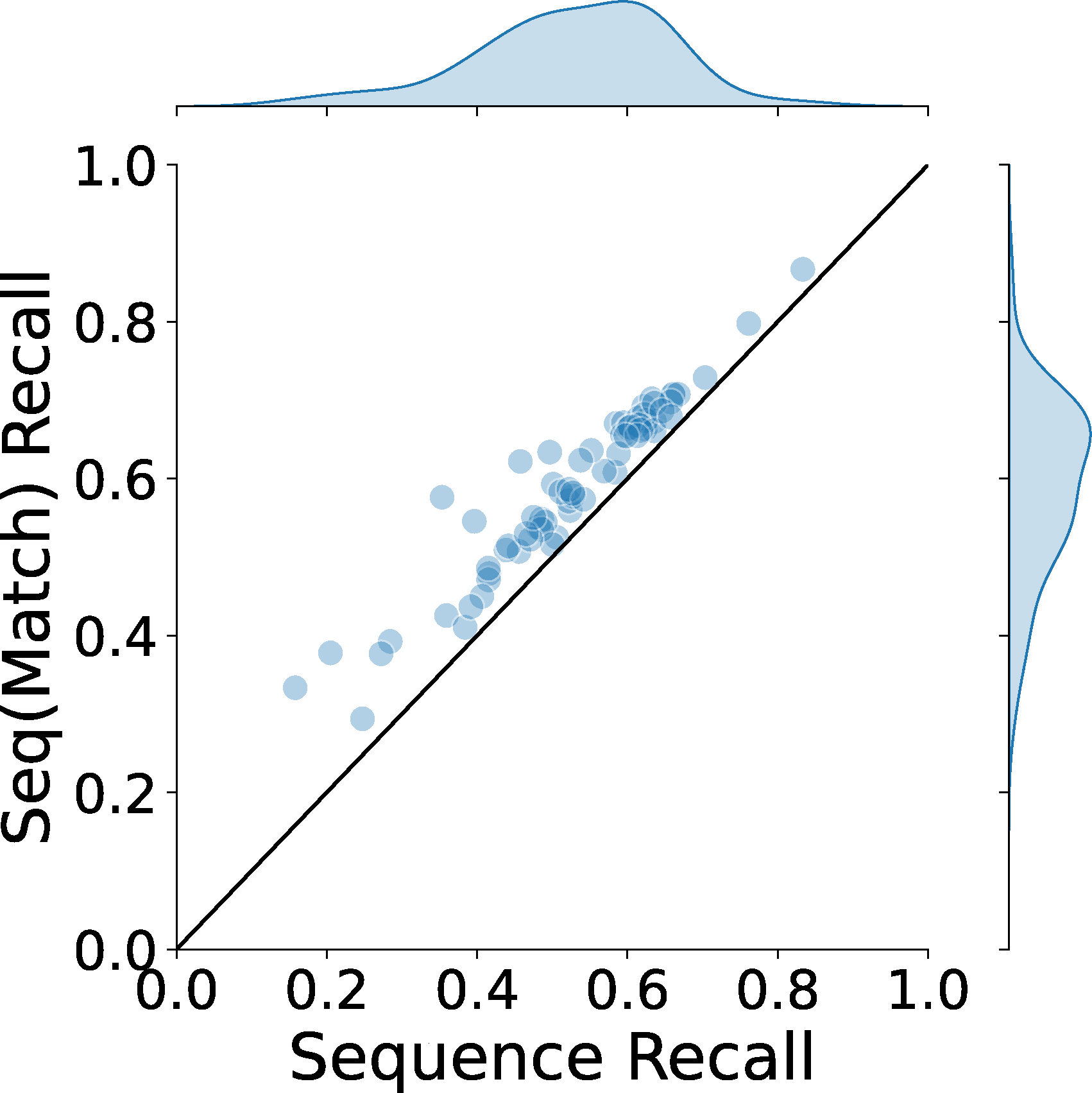
Sequence recall (match) only considers nucleotides in the reference structure that have a corresponding nucleotide in the model (an average atom pair distance of less than 5 Å).
Extended Data 7. Sequence match relative to the map resolution.
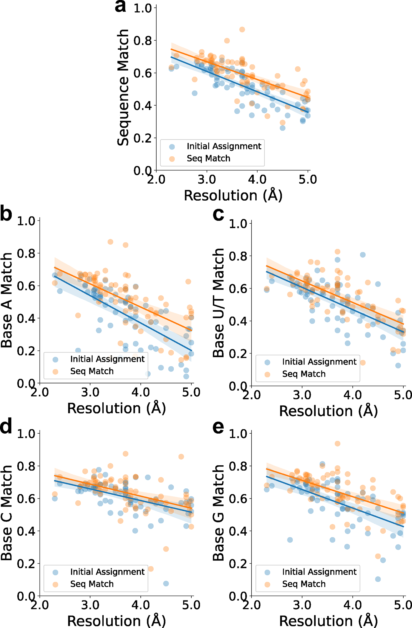
To compute sequence match, first we identified a nucleotide in the model that corresponds to each nucleotide in the reference structure by assigning the nucleotide in the model that has the closest average atom distance, then checked if the bases are identical or not. Sequence match only considers nucleotides in the reference structure that have a corresponding nucleotide in the model (an average atom pair distance of less than 5 Å). In this figure, we compared sequence match of the initial assignment and after the sequence alignment. The initial assignment considers the base type obtained by the base predictions at base nodes of the atomic structures being developed. The initial assignment here is different from the base moiety accuracy reported in Fig. 2a and Extended Data 5 because Fig. 2a and Extended Data 5 concern initial grid-based accuracy of bases by deep learning while the initial sequence assignment here considers accuracy of the base assignment in the modeled tertiary structure, where the base positions are determined in consideration of other atoms in the nucleic acids including phosphate and sugar positions. Seq Match is the reassigned base type by sequence assignment to backbone paths.
a. Overall sequence match. For initial assignment, the equation of regression line is (Pearson correlation coefficient: −0.782, p-value: 3.380e-15, standard error:0.012). For seq match, the equation of regression line is (Pearson correlation coefficient: −0.684, p-value: 1.230e-10, standard error:0.014). b. Sequence match of Adenine (A) relative to the map resolution. For initial assignment, the equation of regression line is (Pearson correlation coefficient: −0.684, p-value: 1.307e-11, standard error:0.022). For seq match, the equation of regression line is (Pearson correlation coefficient: −0.591, p-value: 1.127e-7, standard error:0.024). c. Sequence match of Uracil/Thymine (U/T). For initial assignment, the equation of regression line is (Pearson correlation coefficient: −0.671, p-value: 3.771e-10, standard error:0.019). For seq match, the equation of regression line is (Pearson correlation coefficient: −0.680, p-value: 1.881e-10, standard error:0.018). c. Sequence match of Cytosine (C). For initial assignment, the equation of regression line is (Pearson correlation coefficient: −0.482, p-value: 3.141e-8, standard error:0.016). For seq match, the equation of regression line is (Pearson correlation coefficient: −0.452, p-value: 1.095e-4, standard error:0.018). d. Sequence match of Guanine (G). For initial assignment, the equation of regression line is (Pearson correlation coefficient: −0.578, p-value: 2.381e-7, standard error:0.020). For seq match, the equation of regression line is (Pearson correlation coefficient: −0.595, p-value: 9.017e-8, standard error:0.017).
Extended Data 8. The number of atom clashes before and after the structure refinement.
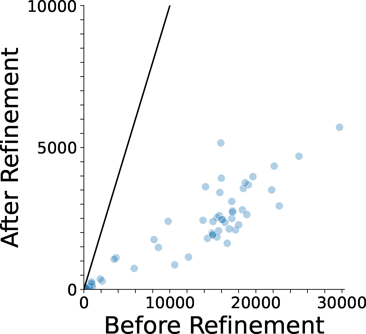
An atom clash is defined as heavy atom pairs closer than 3.0 Å. The line shown is .
Extended Data 9. Examples of modeled atomic structure by CryoREAD for experimental maps without full atomic structures.
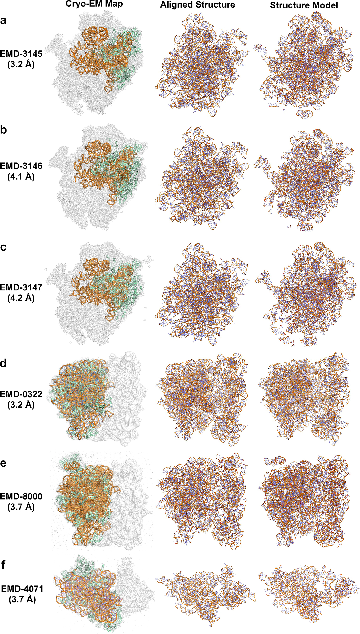
Detailed Evaluation Results are shown in Supplementary Table 3. In this figure, from left to right, the 3 columns correspond to 1) EM map and its corresponding structure; 2) showing only RNA structures in the map. In addition to the RNA structure modeled by the authors, we also shown here homologous structures of missing RNAs in the map, which we searched by BLAST 1. 3) the atomic structure model by CryoREAD. a. the initial Shwachman-Bodian-Diamond syndrome (SBDS) protein closed state of the nascent 60S ribosomal subunit (EMD-3145, PDB-ID: 5AN9, Resolution: 3.3 Å; protein lengths: 1905 aa; RNA length: 1162 nt): Backbone recall: 0.888; Sequence match: 0.696. Identified homologous structure (PDB-ID: 5XXB, RNA length: 3352 nt, Sequence Identity: 84.3%, RMSD: 1.2 Å): Backbone recall: 0.832. b. the SBDS open state of the nascent 60S ribosomal subunit (EMD-3146, PDB-ID: 5ANB, Resolution: 4.1 Å; protein lengths: 3025 aa; RNA length: 1162 nt): Backbone recall: 0.871; Sequence match: 0.544. Identified homologous RNA structure (PDB-ID: 5XXB, RNA length: 3352 nt, Sequence Identity: 84.3%, RMSD: 1.3 Å): Backbone recall: 0.821. c. the ELF1 accommodated state of the nascent 60S ribosomal subunit (EMD-3147, PDB-ID: 5ANC, Resolution: 4.2 Å; protein lengths: 2801 aa; RNA length: 1162 nt): Backbone recall: 0.881; Sequence match: 0.535. Identified homologous structure (PDB-ID: 5XXB, RNA length: 3352 nt, Sequence Identity: 84.3%, RMSD: 1.3 Å): Backbone recall: 0.804. d. TnaC-stalled ribosome complex with the titin I27 domain folding close to the ribosomal exit tunnel (EMD-0322, PDB-ID: 6I0Y, Resolution: 3.2 Å; protein lengths: 3552 aa; RNA length: 3049 nt): Backbone recall: 0.901; Sequence match: 0.632. Identified homologous RNA structure (PDB-ID: 7D80, RNA length: 4761 nt, Sequence Identity: 100%, RMSD: 1.2 Å): Backbone recall: 0.834. e. RNC-SRP-SR complex early state (EMD-8000, PDB-ID: 5GAD, Resolution: 3.7 Å; protein lengths: 4087 aa; RNA length: 3049 nt): Backbone recall: 0.914; Sequence match: 0.655. Identified homologous structure (PDB-ID: 7D80, RNA length: 4761 nt, Sequence Identity: 100%, RMSD: 1.0 Å): Backbone recall: 0.847. f. Structure of the 40S ABCE1 post-splitting complex (EMD-4071, PDB-ID: 5LL6, Resolution: 3.9 Å; protein lengths: 3429 aa; RNA length: 1325 nt): Backbone recall: 0.856; Sequence match: 0.586. Identified homologous structure (PDB-ID: 7OSM, RNA length: 1740 nt, Sequence Identity: 99%, RMSD: 1.0 Å): Backbone recall: 0.784.
In Extended Data 9, we show cases where only a part of the structures in an EM map was modelled by authors. They are maps from three different sets of EM maps of ribosomal subunits. The first set (panel a-c) includes three different states of eIF6 release from the nascent 60S ribosomal subunit 2 of Dictyostelium discoideum, where only part of 26S ribosomal unit is modeled by the authors. The second set (panel d-e) presents two different forms of 70S ribosomal subunit 3 of Escherichia coli, where the authors only modeled 50S ribosomal subunit but 30S ribosomal subunit was left unmodelled. The third example (panel f) is 40S ribosomal subunit of Saccharomyces cerevisiae, where only part of 18S ribosomal RNA was modeled. We filled the missing RNA structure in the maps with homologous RNA structure found by BLAST 1 against PDB. Sequence identities of the identified RNAs were 84.3% to 100%. CryoREAD models for the missing RNA structures had backbone recall of 0.784 to 0.847, when the homologous structures were considered as reference. Backbone recall of CryoREAD models for RNAs with authors’ model was from 0.856 to 0.914.
Extended Data 10. Structure model evaluation on the 68 experimental EM maps with Phenix.
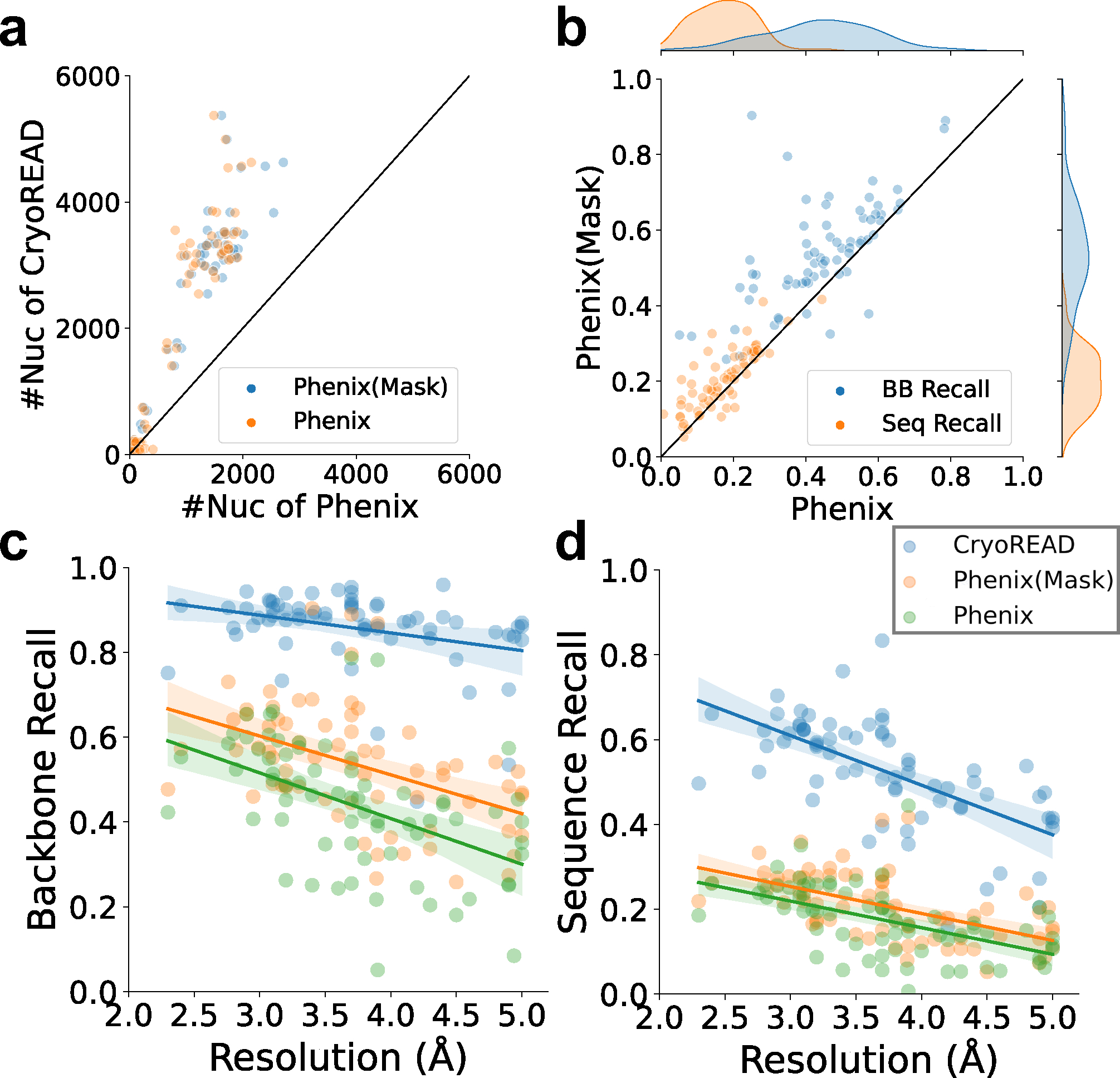
a, the number of nucleotides modelled by Phenix map_to_model and CryoREAD. For Phenix results, two models were generated. Models from map regions that are predicted to include nucleic acid atoms (Phenix (Mask), blue) and models that were built from the entire map (Phenix, orange). b, comparison of backbone atom/sequence recall of Phenix (Mask) and Phenix. c, backbone atom recalls of Phenix (Mask), Phenix, and CryoREAD relative to map resolution. For CryoREAD, the equation of regression line is (Pearson correlation coefficient: −0.320, p-value: 0.008, standard error:0.015). For Phenix(Mask), the equation of regression line is (Pearson correlation coefficient: −0.445, p-value: 1.456e-4, standard error:0.023). For Phenix, the equation of regression line is (Pearson correlation coefficient: −0.492, p-value: 2.006e-5, standard error:0.023). d, sequence recalls of Phenix (Mask), Phenix and CryoREAD relative to map resolution. For CryoREAD, the equation of regression line is (Pearson correlation coefficient: −0.632, p-value: 7.280e-9, standard error:0.017). For Phenix(Mask), the equation of regression line is (Pearson correlation coefficient: −0.550, p-value: 1.190e-6, standard error:0.012). For Phenix, the equation of regression line is (Pearson correlation coefficient: −0.525, p-value: 4.254e-6, standard error:0.013).
Supplementary Material
Acknowledgments
The authors thank Jacob C. Verburgt, Harini Kannan, Anika Jain, Charles Christoffer for their help in literature search, discussion, and proofreading. The authors also thank Jessica A. Nash, Sam Ellis and Jing Chen’s suggestion for optimizing the released software. This work was partly supported by the National Institutes of Health (R01GM133840, 3R01 GM133840-02S1) and the National Science Foundation (DMS2151678, DBI2003635, CMMI1825941, MCB2146026, and MCB1925643). XW is recipient of the MolSSI graduate fellowship.
Footnotes
Competing Interests Statement
The authors declare that there are no competing interests.
Code Availability
The source code of CryoREAD is made available at https://github.com/kiharalab/CryoREAD41. The webserver is available at https://em.kiharalab.org/algorithm/CryoREAD, where user can simply upload the map and get the structures without installment. User can also on Google Colab Notebook Webserver at https://bit.ly/CryoREAD. A detailed tutorial for CryoREAD is available at https://kiharalab.org/emsuites/cryoread.php.
Data Availability
The entries of the maps and corresponding structure models utilized in this study are provided in Supplementary Tables 1 and 4. The experimental EM maps utilized can be downloaded from EMDB (https://www.emdataresource.org/). The corresponding experimental determined structures utilized can be downloaded from RCSB (https://www.rcsb.org/). The modeled structure by CryoREAD is available at https://doi.org/10.5281/zenodo.8274164.
References
- 1.Warner KD, Hajdin CE & Weeks KM Principles for targeting RNA with drug-like small molecules. Nature reviews Drug discovery 17, 547–558 (2018). [DOI] [PMC free article] [PubMed] [Google Scholar]
- 2.Huang P-S, Boyken SE & Baker D The coming of age of de novo protein design. Nature 537, 320–327 (2016). [DOI] [PubMed] [Google Scholar]
- 3.Churkin A et al. Design of RNAs: comparing programs for inverse RNA folding. Briefings in bioinformatics 19, 350–358 (2018). [DOI] [PMC free article] [PubMed] [Google Scholar]
- 4.Berman HM et al. The protein data bank. Nucleic acids research 28, 235–242 (2000). [DOI] [PMC free article] [PubMed] [Google Scholar]
- 5.Emsley P, Lohkamp B, Scott WG & Cowtan K Features and development of Coot. Acta Crystallographica Section D: Biological Crystallography 66, 486–501 (2010). [DOI] [PMC free article] [PubMed] [Google Scholar]
- 6.Liebschner D et al. Macromolecular structure determination using X-rays, neutrons and electrons: recent developments in Phenix. Acta Crystallographica Section D: Structural Biology 75, 861–877 (2019). [DOI] [PMC free article] [PubMed] [Google Scholar]
- 7.Winn MD et al. Overview of the CCP4 suite and current developments. Acta Crystallographica Section D: Biological Crystallography 67, 235–242 (2011). [DOI] [PMC free article] [PubMed] [Google Scholar]
- 8.Alnabati E & Kihara D Advances in Structure Modeling Methods for Cryo-Electron Microscopy Maps. Molecules 25, 82 (2020). [DOI] [PMC free article] [PubMed] [Google Scholar]
- 9.Pfab J, Phan NM & Si D DeepTracer for fast de novo cryo-EM protein structure modeling and special studies on CoV-related complexes. Proceedings of the National Academy of Sciences 118 (2021). [DOI] [PMC free article] [PubMed] [Google Scholar]
- 10.Terashi G & Kihara D De novo main-chain modeling for EM maps using MAINMAST. Nature Communications 9, 1618 (2018). [DOI] [PMC free article] [PubMed] [Google Scholar]
- 11.Maddhuri Venkata Subramaniya SR, Terashi G & Kihara D Protein secondary structure detection in intermediate-resolution cryo-EM maps using deep learning. Nature Methods 16, 911–917, doi: 10.1038/s41592-019-0500-1 (2019). [DOI] [PMC free article] [PubMed] [Google Scholar]
- 12.Song Y et al. High-resolution comparative modeling with RosettaCM. Structure 21, 1735–1742 (2013). [DOI] [PMC free article] [PubMed] [Google Scholar]
- 13.Emsley P & Cowtan K Coot: model-building tools for molecular graphics. Acta crystallographica section D: biological crystallography 60, 2126–2132 (2004). [DOI] [PubMed] [Google Scholar]
- 14.Pettersen EF et al. UCSF Chimera—a visualization system for exploratory research and analysis. Journal of computational chemistry 25, 1605–1612 (2004). [DOI] [PubMed] [Google Scholar]
- 15.Schlick T & Pyle AM Opportunities and challenges in RNA structural modeling and design. Biophysical journal 113, 225–234 (2017). [DOI] [PMC free article] [PubMed] [Google Scholar]
- 16.Keating KS & Pyle AM RCrane: semi-automated RNA model building. Acta Crystallographica Section D: Biological Crystallography 68, 985–995 (2012). [DOI] [PMC free article] [PubMed] [Google Scholar]
- 17.Kappel K et al. Accelerated cryo-EM-guided determination of three-dimensional RNA-only structures. Nature methods 17, 699–707 (2020). [DOI] [PMC free article] [PubMed] [Google Scholar]
- 18.Huang H et al. in ICASSP 2020–2020 IEEE International Conference on Acoustics, Speech and Signal Processing (ICASSP). 1055–1059 (IEEE; ). [DOI] [PMC free article] [PubMed] [Google Scholar]
- 19.Ronneberger O, Fischer P & Brox T in International Conference on Medical image computing and computer-assisted intervention. 234–241 (Springer; ). [Google Scholar]
- 20.Carreira-Perpinan MA in 2006 IEEE Computer Society Conference on Computer Vision and Pattern Recognition (CVPR’06). 1160–1167 (IEEE; ). [Google Scholar]
- 21.Psaraftis HN Dynamic vehicle routing problems. Vehicle routing: Methods and studies 16, 223–248 (1988). [Google Scholar]
- 22.Rossi F, Van Beek P & Walsh T Handbook of constraint programming. (Elsevier, 2006). [Google Scholar]
- 23.Afonine PV et al. Real-space refinement in PHENIX for cryo-EM and crystallography. Acta Crystallographica Section D: Biological Crystallography 74 (2018). [DOI] [PMC free article] [PubMed] [Google Scholar]
- 24.Wang X et al. Detecting protein and DNA/RNA structures in cryo-EM maps of intermediate resolution using deep learning. Nature communications 12, 1–9 (2021). [DOI] [PMC free article] [PubMed] [Google Scholar]
- 25.Kim M-S et al. Cracking the DNA code for V (D) J recombination. Molecular cell 70, 358–370. e354 (2018). [DOI] [PMC free article] [PubMed] [Google Scholar]
- 26.Grimm C et al. Structural basis of poxvirus transcription: vaccinia RNA polymerase complexes. Cell 179, 1537–1550. e1519 (2019). [DOI] [PubMed] [Google Scholar]
- 27.Li S et al. Structural basis of amino acid surveillance by higher-order tRNA-mRNA interactions. Nature structural & molecular biology 26, 1094–1105 (2019). [DOI] [PMC free article] [PubMed] [Google Scholar]
- 28.Nikolay R et al. Snapshots of native pre-50S ribosomes reveal a biogenesis factor network and evolutionary specialization. Molecular Cell 81, 1200–1215. e1209 (2021). [DOI] [PubMed] [Google Scholar]
- 29.Shi M et al. SARS-CoV-2 Nsp1 suppresses host but not viral translation through a bipartite mechanism. BioRxiv (2020). [Google Scholar]
- 30.Schubert K et al. SARS-CoV-2 Nsp1 binds the ribosomal mRNA channel to inhibit translation. Nature structural & molecular biology 27, 959–966 (2020). [DOI] [PubMed] [Google Scholar]
- 31.Thoms M et al. Structural basis for translational shutdown and immune evasion by the Nsp1 protein of SARS-CoV-2. Science 369, 1249–1255 (2020). [DOI] [PMC free article] [PubMed] [Google Scholar]
- 32.Naydenova K et al. Structure of the SARS-CoV-2 RNA-dependent RNA polymerase in the presence of favipiravir-RTP. Proceedings of the National Academy of Sciences 118, e2021946118 (2021). [DOI] [PMC free article] [PubMed] [Google Scholar]
- 33.Wang Q et al. Structural basis for RNA replication by the SARS-CoV-2 polymerase. Cell 182, 417–428. e413 (2020). [DOI] [PMC free article] [PubMed] [Google Scholar]
- 34.Chen J et al. Structural basis for helicase-polymerase coupling in the SARS-CoV-2 replication-transcription complex. Cell 182, 1560–1573. e1513 (2020). [DOI] [PMC free article] [PubMed] [Google Scholar]
- 35.Terwilliger TC, Adams PD, Afonine PV & Sobolev OV A fully automatic method yielding initial models from high-resolution cryo-electron microscopy maps. Nature methods 15, 905–908 (2018). [DOI] [PMC free article] [PubMed] [Google Scholar]
- 36.Sudre CH, Li W, Vercauteren T, Ourselin S & Jorge Cardoso M in Deep learning in medical image analysis and multimodal learning for clinical decision support 240–248 (Springer, 2017). [DOI] [PMC free article] [PubMed] [Google Scholar]
- 37.Kingma DP & Ba J in International Conference on Learning Representations (2015). [Google Scholar]
- 38.Fukunaga K & Hostetler L The estimation of the gradient of a density function, with applications in pattern recognition. IEEE Transactions on information theory 21, 32–40 (1975). [Google Scholar]
- 39.Toth P & Vigo D The vehicle routing problem. (SIAM, 2002). [Google Scholar]
- 40.Lorenz R et al. ViennaRNA Package 2.0. Algorithms for molecular biology 6, 1–14 (2011). [DOI] [PMC free article] [PubMed] [Google Scholar]
- 41.Wang X, Terashi G & Kihara D CryoREAD: De novo structure modeling for nucleic acids in cryo-EM maps using deep learning. https://github.com/kiharalab/CryoREAD https://doi.org/10.5281/zenodo.8274181. [DOI] [PMC free article] [PubMed] [Google Scholar]
Reference
- 1.Altschul SF, Gish W, Miller W, Myers EW & Lipman DJ Basic local alignment search tool. Journal of molecular biology 215, 403–410 (1990). [DOI] [PubMed] [Google Scholar]
- 2.Weis F et al. Mechanism of eIF6 release from the nascent 60S ribosomal subunit. Nature structural & molecular biology 22, 914–919 (2015). [DOI] [PMC free article] [PubMed] [Google Scholar]
- 3.Jomaa A, Boehringer D, Leibundgut M & Ban N Structures of the E. coli translating ribosome with SRP and its receptor and with the translocon. Nature communications 7, 1–9 (2016). [DOI] [PMC free article] [PubMed] [Google Scholar]
Associated Data
This section collects any data citations, data availability statements, or supplementary materials included in this article.
Supplementary Materials
Data Availability Statement
The entries of the maps and corresponding structure models utilized in this study are provided in Supplementary Tables 1 and 4. The experimental EM maps utilized can be downloaded from EMDB (https://www.emdataresource.org/). The corresponding experimental determined structures utilized can be downloaded from RCSB (https://www.rcsb.org/). The modeled structure by CryoREAD is available at https://doi.org/10.5281/zenodo.8274164.


