Correction of phase offset errors and quantification of background noise, signal-to-noise ratio, and encoded-displacement uncertainty on DENSE MRI for kinematics of the descending thoracic and abdominal aorta

Abstract

Displacement encoding with stimulated echoes (DENSE) MRI is a phase contrast technique that allows the encoding of tissue displacement into the phase of the magnetic resonance signal. Recent developments in this technique allow the imaging of relatively thin structures such as the aortic wall. Quantifying background noise associated to DENSE MRI is required to assess the uncertainty of derived displacement measurements and for the design and implementation of adequate noise-reduction techniques. Although noise and error management of cardiac DENSE MRI has been previously studied, developments for aortic applications are scarce. Herein, we evaluate the noise and uncertainty of DENSE MRI scans at three different locations along the descending aorta: the distal aortic arch (DAA), the descending thoracic aorta (DTA), and infrarenal abdominal aorta (IAA). Additionally, we analyze three datasets from in vitro validation experiments with polyvinyl alcohol phantoms. We implement and evaluate the effectiveness of an offset-error correction algorithm and noise filtering techniques on DENSE MRI for aortic motion applications. Our results show that the phase signal of pixels composing the static background was normally distributed, centered on average at 0.003±0.02 rad and −0.02±0.024 rad for each phase directions, suggesting that background noise is random, isotropic, and DENSE MRI has little offset errors. However, background signal noise significantly increased with elapsed time of the cardiac cycle; and was spatially heterogeneous consistently increased towards the anterior space. Background noise showed no significant differences between the 3 aortic locations and the in vitro experiments. However, SNR depended on the displacement of the region of interest, in consequence it was found significantly larger at DAA (16.7±8.5, p=0.003) and DTA (15.4±7.6, p=0.008) than at the IAA (8.0±4.1), but Journal Pre-proof not significantly different than the SNR of in vitro experiments (8.0±3.7), and had an overall average of 13±7. The applied methods significantly reduced the offset error and effect of noise on the estimation of encoded displacements. Finally, this analysis suggests that the implemented DENSE MRI protocol is adequate to assess the motion of healthy human aortas. However, the relative effect of noise increased considerably on the analysis of an ageing or diseased aortas with impaired mobility, calling for further analyses on pathologically stiffened aortas.

1. Introduction

Displacement encoding with stimulated echoes (DENSE) magnetic resonance imaging (MRI) is a technique that encodes tissue displacement into the magnetic resonance signal phase [1]. DENSE MRI has primarily been utilized for the assessment of myocardial motion and applied to the identification of markers for early cardiac dysfunction [2,3], the response to cardiac resynchronization therapy [4,5], and the detection of transmural infarction [6,7]. Notably, recent advances in spiral k-space sampling DENSE MRI with custom noise-reducing post-processing allow the imaging and kinematic analysis of thinner structures, such as the aortic wall [8–10]. These improvements have even shown the potential to assess radial, circumferential, and shear strains on the thin walls of large arteries [11]. However, the aortic wall is significantly thinner than the myocardium and associated with smaller displacements, making these measurements more sensitive to the effect of MRI signal noise and error.

Effects from concomitant fields, non-linearity of magnetic gradients, eddy currents, and mechanical field oscillations are potential sources of noise and error on MRI-derived measurements [12]. Signal noise introduces uncertainty to DENSE MRI-derived measures of displacement, strain, and change in volume [13]. The signal-to-noise ratio (SNR) is a commonly employed measure to assess how image-based metrics could be affected by signal noise, typically defined as the ratio of the averaged signal within the region of interest (ROI) to the signal noise. A threshold of SNR<2 has been proposed to determine if an MRI signal is biased due to noise [14]. Noise can be quantified in vivo by measuring the temporal variation of the signal from static structures (or background). This approach does not require additional scan time, dedicated hardware, or the use of phantoms [15].

The accuracy of DENSE MRI has been validated in both cardiac and aortic phantoms by comparison to tracking of physical markers on in vitro experimental setups [16–19]. However, fewer studies have specifically evaluated the signal noise and potential errors of DENSE MRI. Previous studies of cardiac and ventricular kinematics using DENSE MRI have reported SNR estimations ranging from 10 to 35, a magnitude that depends on the subject, the specific DENSE MRI scanning sequence, and scanning parameters such as magnetization energy, encoding frequency, and flip angle [18,20–22].

To the authors’ knowledge, no prior study has addressed the estimation of signal noise and error for aortic DENSE MRI, which is critical, given the relatively lower thickness and displacement of the aortic wall in comparison with the myocardium. Therefore, the goal of this study was to perform a detailed analysis of background noise, SNR, and uncertainty of the encoded displacement field from a 2D cine DENSE sequence for the study of human aortic kinematics, and to evaluate the effectiveness of correction methods for offset error and noise. The analysis is performed on datasets collected from healthy-adult volunteers at three locations of the descending aorta – distal aortic arch (DAA), descending thoracic aorta (DTA), and infrarenal abdominal aorta (IAA) - and on in vitro setups with polyvinyl alcohol (PVA) phantoms.

2. Methods

2.1. In vivo study

All imaging data were retrospectively collected from previously published studies [9]. The three aortic locations under study were the IAA at the level of the fourth portion of the duodenum, the DTA at the level of the mitral valve, and the DAA distal to the left subclavian artery (Figure 1a). Nine datasets were analyzed for each aortic location for a total of 27 cases of study. Each dataset was acquired from a different volunteer except for four pairs of DAA and DTA datasets collected from the same individuals (Table 1). Cardiac-gated DENSE MRI were acquired on either a 3 Tesla Siemens Trio or Prisma Fit Scanner (Siemens Healthineers, Erlangen, Germany) during free-breathing with a respiratory navigator. Spiral k-space sampling and fat suppression were utilized. Relevant imaging parameters include: repetition time (TR) of 16 ms, time to echo (TE) of 1.21 ms, in-plane displacement encoding frequency $\left(k_e\right)$ in the range of 0.17–0.25 cyc/mm, 18 spiral interleaves, 2 interleaves per heartbeat, 4 signal averages, slice thickness 8 mm, and isotropic pixel sizes of 1.34 ± 0.08 mm (Table 1). The time series consisted of 18 temporal acquisitions separated by approximately 32 ms to ensure temporal coverage from the initiation of cardiac systole through local aortic systole for the entire length of the aorta.

Figure 1.

a) Location of scan planes from in vivo studies. b) Representative DICOM images of magnitude, phase x, and phase y at systole. c) Representative segmentations of the aortic wall with DENSE MRI-derived pixel-wise displacement fields.

Table 1.

DENSE MRI parameters and case-specific results

Group	#	Age	FOV [mm × mm]	Pixel size [mm]	$k_e\left[\frac{cycle}{mm}\right]$	Background phase signal range. Offset error ± Mean SD		Background phase signal variation over time or mean noise		SWR	$\bar{d}\left[mm\right]$	${\bar{D}}_{wall}\left[mm\right]$
						${\bar{\mu }}_x\pm {\bar{\sigma }}_x\left[rad\right]$	${\stackrel{-}{\mu }}_y\pm {\bar{\sigma }}_y[rad]$	${\bar{\tau }}_x\pm SD\left[rad\right]$	${\bar{\tau }}_y\pm SD\left[rad\right]$
DAA	1	19	380×380	1.2667	0.25	0.029 ± 0.072	0.031 ± 0.083	0.045 ± 0.014	0.045 ± 0.015	25	0.06	3.1 ± 1.1
	2	23	340×340	1.3281	0.25	0.011 ± 0.124	0.0165 ± 0.079	0.051 ± 0.017	0.048 ± 0.018	24	0.07	2.9 ± 1.2
	3	26	380×380	1.2667	0.25	0.023 ± 0.059	0.006 ± 0.071	0.044 ± 0.014	0.048 ± 0.016	20	0.41	1.8 ± 0.5
	4	37	380×380	1.2667	0.25	0.0063 ± 0.079	0.0018 ± 0.083	0.052 ± 0.019	0.053 ± 0.019	15	0.35	1.7 ± 0.7
	5	38	360×360	1.2857	0.18	0.0004 ± 0.1031	−0.047 ± 0.134	0.066 ± 0.025	0.072 ± 0.026	17	0.12	2.5 ± 0.5
	6	56	380×380	1.4844	0.16	0.032 ± 0.126	−0.035 ± 0.138	0.066 ± 0.019	0.068 ± 0.022	14	0.08	1.8 ± 0.9
	7	58	340×340	1.3281	0.18	0.0097 ± 0.143	−0.013 ± 0.114	0.082 ± 0.021	0.079 ± 0.022	7	0.07	1.2 ± 0.5
	8	58	340×340	1.3281	0.25	0.014 ± 0.117	−0.071 ± 0.125	0.069 ± 0.023	0.076 ± 0.026	15	0.07	2.3 ± 0.7
	9	58	380×380	1.2667	0.17	0.045 ± 0.130	0.0064 ± 0.072	0.087 ± 0.025	0.085 ± 0.027	15	0.17	2.2 ± 0.5
DTA	10	22	340×340	1.3281	0.25	−0.032 ± 0.148	−0.102 ± 0.154	0.061 ± 0.028	0.071 ± 0.045	14	0.06	1.6 ± 0.7
	11	23	340×340	1.3281	0.25	−0.0002 ± 0.0909	−0.019 ± 0.136	0.055 ± 0.021	0.062 ± 0.028	28	0.05	2.5 ± 0.8
	12	23	340×340	1.3281	0.25	−0.015 ± 0.099	−0.032 ± 0.102	0.047 ± 0.015	0.050 ± 0.021	25	0.05	2.6 ± 1.0
	13	24	340×340	1.3281	0.25	−0.006 ± 0.105	0.004 ± 0.134	0.070 ± 0.032	0.070 ± 0.051	14	0.07	2.0 ± 0.7
	14	26	340×340	1.3281	0.25	−0.022 ± 0.078	−0.034 ± 0.086	0.056 ± 0.023	0.059 ± 0.024	11	0.08	1.2 ± 0.7
	15	30	340×340	1.3281	0.25	−0.11 ± 0.087	0.004 ± 0.135	0.047 ± 0.018	0.051 ± 0.021	21	0.07	2.3 ± 1.2
	16	56	340×340	1.3281	0.25	0.065 ± 0.147	−0.049 ± 0.159	0.064 ± 0.020	0.082 ± 0.026	7	0.06	1.3 ± 0.8
	17	58	340×340	1.3281	0.25	0.102 ± 0.139	0.0114 ± 0.096	0.059 ± 0.017	0.062 ± 0.022	12	0.06	1.6 ± 1.0
	18	59	340×340	1.3281	0.25	0.024 ± 0.114	−0.032 ± 0.131	0.058 ± 0.022	0.067 ± 0.031	9	0.06	1.2 ± 0.5
IAA	19	18	340×340	1.6346	0.25	0.002 ± 0.108	0.011 ± 0.134	0.058 ± 0.026	0.067 ± 0.029	9	0.13	1.1 ± 0.6
	20	23	340×340	1.3125	0.25	0.024 ± 0.182	0.007 ± 0.178	0.079 ± 0.037	0.089 ± 0.043	10	0.38	1.7 ± 0.8
	21	27	340×340	1.3281	0.25	0.009 ± 0.155	−0.001 ± 0.165	0.100 ± 0.038	0.108 ± 0.043	9	0.10	2.1 ± 0.8
	22	31	340×340	1.3125	0.25	0.009 ± 0.077	−0.044 ± 0.101	0.049 ± 0.014	0.057 ± 0.016	16	0.10	1.8 ± 0.6
	23	32	350×350	1.3672	0.25	0.003 ± 0.210	−0.021 ± 0.239	0.131 ± 0.081	0.139 ± 0.099	12	0.17	1.4 ± 0.8
	24	36	340×340	1.3125	0.25	0.014 ± 0.173	0.048 ± 0.259	0.082 ± 0.034	0.096 ± 0.039	6	0.07	0.7 ± 0.3
	25	42	340×340	1.6154	0.25	−0.007 ± 0.163	−0.047 ± 0.214	0.094 ± 0.039	0.110 ± 0.051	7	0.13	1.7 ± 0.4
	26	50	340×340	1.3281	0.25	−0.003 ± 0.0171	0.006 ± 0.205	0.088 ± 0.037	0.096 ± 0.044	7	0.08	1.1 ± 0.3
	27	65	340×340	1.3281	0.25	0.023 ± 0.145	−0.025 ± 0.149	0.084 ± 0.029	0.084 ± 0.031	5	0.06	1.0 ± 0.2
Invitro	28	--	340×340	1.3281	0.25	0.036 ± 0.068	−0.067 ± 0.064	0.042 ± 0.014	0.046 ± 0.015	5	0.05	0.9 ± 0.2
	29	--	340×340	1.3281	0.25	−0.011 ± 0.039	−0.043 ± 0.041	0.072 ± 0.061	0.57 ± 0.043	10	0.04	1.2 ± 0.5
	30	--	340×340	1.3281	0.25	−0.044 ± 0.039	−0.059 ± 0.034	0.058 ± 0.35	0.051 ± 0.028	10	0.12	1.1 ± 0.5

Legend:

${\stackrel{-}{\mathit{\mu }}}_{\mathit{x}},{\stackrel{-}{\mathit{\mu }}}_{\mathit{x}}$: Mean offset error or overall phase mean of the background pixels for phase encoding directions x and y respectively.

${\stackrel{\mathit{‾}}{\mathit{\sigma }}}_{\mathit{x}},{\stackrel{\mathit{‾}}{\mathit{\sigma }}}_{\mathit{y}}$: Standard deviation of phase of the background for phase encoding directions x and y respectively.

${\stackrel{-}{\mathit{\tau }}}_{\mathit{x}},{\stackrel{-}{\mathit{\tau }}}_{\mathit{y}}$: Mean pixel-wise standard deviation of phase over time or mean noise for phase encoding directions x and y respectively.

${\mathit{k}}_{\mathit{e}}$: Encoding frequency

$\mathit{d}$: Encoded-displacement uncertainty. ${\stackrel{\mathit{‾}}{\mathit{D}}}_{\mathit{w}\mathit{a}\mathit{l}\mathit{l}}$: DENSE-MRI derived mean displacement of the aortic wall. FOV: Field of view. SNR: Signal-to-noise ratio. SD:Standard deviation.

All 2D imaging planes were acquired orthogonal to the local longitudinal axis of the aorta (i.e. imaging plane normal aligned with the lumen centerlines) with a relatively large slice thickness to ameliorate the effect of any small through-plane motions (Figure 1b) [9]. Scanning planes at the DTA and IAA were oriented such that the vertical coordinate $y$ (along pixel rows) was positive towards the posterior of the volunteer. The selection of DAA imaging planes depended on patient-specific curvature of the aortic arch; however, the majority of cases were oriented such that the positive y-direction was oriented towards the anterior chest wall. Image and phase data were rotated and/or mirrored when necessary to match the above-described orientation.

2.2. In vitro study.

Analysis of background noise was also performed on previously published in vitro data from a validation study of DENSE MRI-derived circumferential strain performed with aortic phantoms placed in a flow loop inside the MRI scanner [16]. Briefly, the experiments consisted of the controlled inflation of polyvinyl alcohol (PVA) phantoms with implanted physical markers (nitinol wires) and enriched with gadolinium to improve MRI contrast. Phantoms were regular cylinders of 2 cm inner diameter and 0.2 cm wall thickness submerged in a water pool, and cyclically pressurized with a pulse-pressure of 60 mmHg of amplitude producing diameter changes of 1.1 ± 0.1 mm on average. Three different experimental setups for inflation were tested: free expansion, expansion against a solid flat PVA support block, and expansion against a solid curved PVA support block (Figure 2). Support blocks were employed to promote asymmetric displacement patterns more relatable to the in vivo setting (with the phantoms pushing against and moving away from the support blocks). The in vitro DENSE MRI was performed on a 3T scanner (Prisma Fit, Siemens Medical Systems, Malvern, PA, USA) using a multi-channel body array coil placed over the water-filled chamber containing the phantom model. Imaging parameters were identical to the in vivo DENSE scans, with $k_e=0.25\mathrm{c}\mathrm{y}\mathrm{c}/\mathrm{m}\mathrm{m}$.

Figure 2.

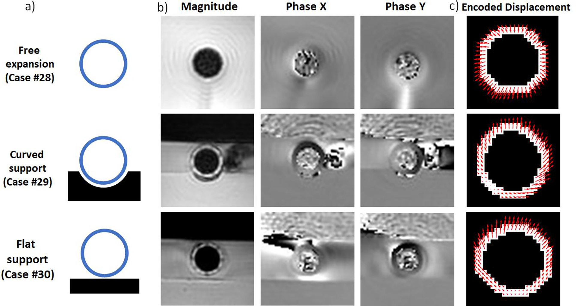
a) Diagram of in vitro validation experiments. b) DICOM images of magnitude, phase x and phase y at maximum inflation (local systole). c) Segmentations of the wall of the phantom with DENSE MRI-derived pixel-wise displacement fields.

2.3. Identification of stationary tissue.

On MRI studies, the background can be defined as voxels that theoretically should emit no signal. For DENSE MRI, the background can be defined as any voxel corresponding to static (non-moving) structures. Segmentation of these static structures was performed by calculating the pixel-wise standard deviation of phase signal over time and selecting the pixels with time-variations of phase below a specific threshold value (Figure 3b,3c). This threshold value was calibrated to each dataset until the automatic segmentation included the skeletal structures but minimal soft tissue for the in vivo cases, and the supporting blocks and the fluid at rest for the in vitro cases. A frame of analysis was defined as a 140×140 pixel window centered at the segmentation of the aortic wall for in vivo studies and a 60×60 pixel window for the in vitro studies to minimize border and artifact effects from the quantification of noise (Figure 3d). Pixel masks of the background were generated for each phase (i.e. encoded motion direction).

Figure 3.

Automatic segmentation of static tissues (background). a) Stack of time-resolved DENSE MRI phase images were processed to obtain the b) pixel-wise distribution of standard deviation of phase over time. c) Histogram of phase standard deviation over time. A threshold is defined to select the pixels with lowest temporal variation of phase to define. c) Segmentation of static structures from selected pixels below the threshold. Top row, representative case of the DTA; bottom row, representative in vitro validation experiment. A frame of analysis is defined around the location of the aortic/phantom cross-section. Note that static structures correspond to the musculoskeletal system in vivo and to the supporting PVA blocks and static fluid away from the phantom in vitro.

2.4. Quantification of phase signal noise on background pixels.

The phase signal of each pixel of the static background randomly oscillates around a mean value such that

$${\varphi }_i\left(x,y,t\right)={\alpha }_i\left(x,y\right)+{\epsilon }_i\left(x,y,t\right),$$ (1)

where ${\varphi }_i(x,y,t)$ is the phase signal in radians, ${\alpha }_i(x,y)$ is the signal mean value over time, ${\epsilon }_i(x,y,t)$ is the random variation of the signal, also defined as the zero-mean noise [15]. Independent variables $x$ and $y$ are the column and row coordinates of the pixel within the scan plane, and $t$ is the elapsed time since encoding. Sub-index $i$ stands for the each of the phase encoding displacement directions $(i=x,y)$ (Figure 4a). In this work, two alternatives are explored to quantify and characterize the random variation of signal ${\epsilon }_i(x,y,t)$ at background pixels. Noise signal intensity was quanitified first, by analyzing the random time-variation on each individual background pixel to quantify noise signal variability (section 2.4.1), and second, by analyzing the signal range over all background pixels at each acquired image or time instant (section 2.4.2).

Figure 4.

Processing of pixel-wise temporal variation of phase. a) Representative time-variation of phase data on a background pixel ${\varphi }_i(x,y,t)$ and graphical representations of pixel-specific offset error ${\alpha }_i(x,y)$, zero-mean random noise ${\epsilon }_i(x,y,t)$, and phase standard deviation over time ${\tau }_i(x,y)$. b) Time-variation of phase data of all background pixels, and graphical representation of mean offset error ${\bar{\alpha }}_i$ and mean random noise ${\bar{\tau }}_i$. The band of phase variability is wider than ${\bar{\alpha }}_i\pm {\bar{\tau }}_i$ due to the variability of pixel-wise offset. c) Spatial distribution of pixel-wise offset error ${\alpha }_i(x,y)$. d) Spatial distribution of pixel-wise noise ${\tau }_i(x,y)$. e) Best-fit surface to pixel-wise spatial distribution of ${\alpha }_i(x,y)$. f) Best-fist surface to pixel-wise spatial distribution of noise ${\tau }_i(x,y)$. g) Probability distribution of ${\alpha }_i(x,y)$ and representation of mean offset error ${\bar{\alpha }}_i$. h) Probability distribution of ${\tau }_i(x,y)$ and representation mean noise ${\bar{\tau }}_i$.

2.4.1. Analysis of pixel-wise time-variation of phase signal on background pixels.

The temporal variations of signal of background pixels ${\epsilon }_i(x,y,t)$ are expected to be random; thus, the standard deviation of the phase signal ${\varphi }_i(x,y,t)$ over time, defined as ${\tau }_i(x,y)$, is a reasonable quantification of the pixel-wise random noise (Figure 4a) [23]. Increasing values of ${\tau }_i(x,y)$ correspond to larger variability of phase data over time, while increasing absolute values of the temporal mean signal ${\alpha }_i(x,y)$ correspond to larger steady offset errors (Figure 4 a). Pixel-wise ${\alpha }_i(x,y)$ and ${\tau }_i(x,y)$ data can be used to generate maps to identify regions affected by larger offset errors and noise. This potential spatial dependence is explored quantitatively by fitting linear planes to ${\alpha }_i(x,y)$ and ${\tau }_i(x,y)$ and analyzing their slopes and correlation indexes. Additionally, mean values of ${\alpha }_i(x,y)$ and ${\tau }_i(x,y)$ of all background pixels can be used to provide an overall representative value of the offset error $\left({\bar{\alpha }}_i\right)$ and the background noise $\left({\bar{\tau }}_i\right)$ for each phase on each dataset.

2.4.2. Analysis of phase signal on background pixels per timestep.

An alternative way to analyze the variability of phase signal in background pixels is to investigate the frequency distribution of ${\varphi }_i(x,y,t)$ of background pixels at each time step. At a given time step $t_j$, pixel-wise phase signal ${\varphi }_i\left(x,y,t_j\right)$ will be distributedaround a mean value, defined as ${\mu }_i\left(t_j\right)$, which corresponds to the pixel-averaged offset error at the time $t_j$. If the distribution is normal, then the standard deviation of the pixelwise phase signal, defined as ${\sigma }_i\left(t_j\right)$, represents a reasonable measure of the range of background signal intensity around the mean at a given time. The range ${\mu }_i\left(t_j\right)\pm {\sigma }_i\left(t_j\right)$ (i.e., one standard deviation above and below the mean) contains about 68% of the surveyed data at time step $t_j$ (Figure 5 b). Larger values of ${\sigma }_i\left(t\right)$ reflect broader ranges of phase signals from the background, and thus the typical signal intensity of noise. This time-resolved information can be used to explore the dependence of pixel-averaged offset error and the most probable range of phase signal of the background over the cardiac cycle that may change depending on the elapsed time since phase-encoding (Figure 5c). Finally, mean values of ${\mu }_i\left(t\right)$ and ${\sigma }_i\left(t\right)$ over time were calculated to provide reasonable estimations of overall offset error ${\bar{\mu }}_i$ and the spread of phase signal of the background background ${\bar{\mu }}_i\pm {\bar{\sigma }}_i$ (Figure 5c,5d).

Figure 5.

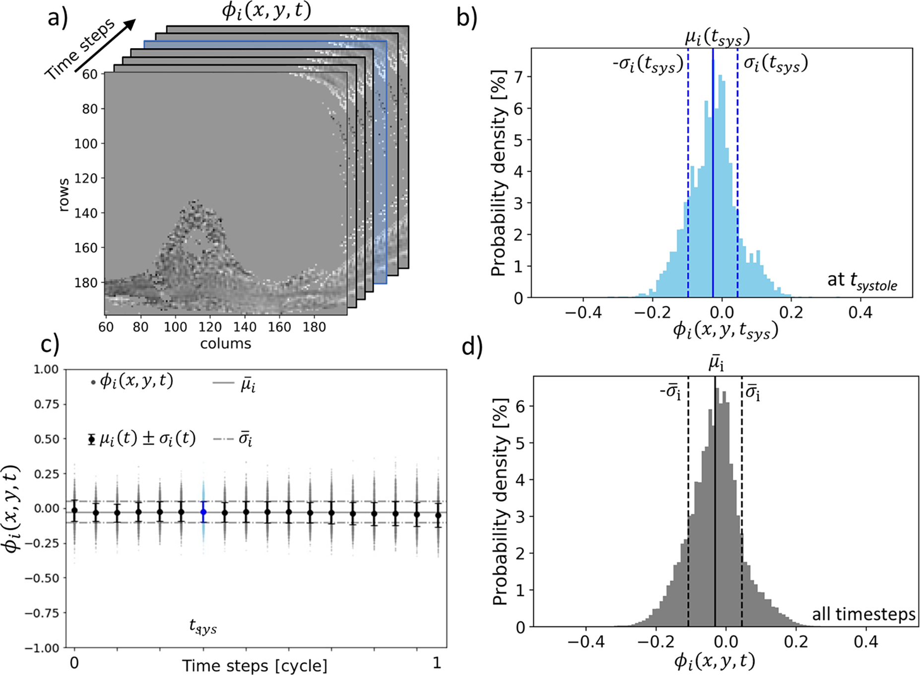
a) Spatial distribution of phase of the background pixels. Statistical analysis of phase data is carried on each timestep. The systolic timestep is highlighted in blue. b) Probability distribution of phase at the systolic timestep and representation of time-specific phase mean $\mu \left(t\right)$ and standard deviation $\sigma \left(t\right)$. c) Pixelspecific phase data (dots), mean and standard deviation of phase for each timestep (whisker plot). The solid horizontal line represents the overall phase mean ${\bar{\mu }}_i$ (equivalent of the mean offset error ${\bar{\alpha }}_i$). Dashed horizontal lines represent the overall phase standard deviation ${\bar{\sigma }}_i$ as a measure of the spread of phase data. d) Probability distribution of phase signal of the background overall time steps. The distribution approaches normality so that the range ${\bar{\mu }}_i\pm {\bar{\sigma }}_i$ encloses about 68% of all background phase signal.

2.5. Phase data and displacement of the aortic wall and phantoms.

Manual segmentation of the aortic wall (or wall of the phantom) with a prescribed two pixel-width thickness was collected from previous studies [10,16]. Phase data was collected for all pixels within the segmented masks. Any aliased pixels were identified, and their phase information was unwrapped, as necessary, with an automatic algorithm previously described elsewhere [18]. Phase data within the wall segmentations was converted to encoded displacements in their corresponding direction $(i=x,y)$ for each segmented pixel using the case-specific encoding frequency (Table 1):

$$D_{{wall}_i}\left(x,y\right)=\frac{{\varphi }_{{wall}_i}\left(x,y,t_j\right)}{2\pi k_e}.$$ (2)

The resulting displacement field was smoothed by a two-step noise-filtering algorithm as described by Wilson et al. [9]. The total pixel-wise displacement was calculated as the vector sum of the directional components. An average value $\left({\bar{D}}_{wall}\right)$ for all pixels within the mask was also obtained to represent the net case-specific aortic (or phantom) motion.

2.6. Displacement uncertainty ($d$) and signal-to-noise ratio (SNR).

Displacement uncertainty was calculated for each case by converting the representative phase noise $\left({\bar{\tau }}_i\right)$ to displacement for each direction $(i=x,y)$

$${\bar{d}}_i=\frac{{\bar{\tau }}_i}{2\pi k_e}.$$ (3)

The total displacement uncertainty was estimated for the mean displacement following the principles of uncertainty propagation as:

$$\bar{d}={\bar{D}}_{wall}\sqrt{2{\left(\frac{{\bar{d}}_x}{{\bar{D}}_{{wall}_x}}\right)}^2+2{\left(\frac{{\bar{d}}_y}{{\bar{D}}_{{wall}_y}}\right)}^2}$$ (4)

SNR was calculated as the average of the absolute value of the pixel-wise phase data within the mask divided by the representative phase noise as follows:

$$SN{R}_i=\frac{{\stackrel{-}{\left|{\varphi }_{{wall}_l}\left(x,y,t_{systole}\right)\right|}}_{ROI}}{{\bar{\tau }}_i}$$ (5)

2.7. Correction of offset error and background noise.

The method proposed by Lankhaar et al. [15] to correct the offset error on velocity-encoding 2D PC MRI measuring blood velocity was employed herein on the DENSE MRI datasets. The method consists of calculating the best-fit plane $\left(A_i(x,y)=a_{2}x+\right.\left.a_{1}y+a_0\right)$ to the spatial distribution of offset error ${\alpha }_i(x,y)$ (Figure 4e), and then subtracting it from the phase data, such that:

$${\varphi }_i^{corr}(x,y,t)={\varphi }_i(x,y,t)-A_i\left(x,y\right)$$ (6)

Because pixel-wise offset error is a mean value over time, the correction surface $A(x,y)$ is independent of time. Then, to verify the effectiveness of the correction method, statistical metrics of the phase signal of the background can be recomputed $\left({\bar{\alpha }}_i^{corr},{\bar{\tau }}_i^{corr},{\bar{\mu }}_i^{corr},{\bar{\sigma }}_i^{corr}\right)$.

2.8. Quantification of the effect of noise on displacement distribution of the aortic wall.

To quantify the effect of noise on the displacement distribution of the aortic wall, random selections from the case-specific noise probability distribution ${\tau }_i(x,y)$ on each phase were converted to displacement noise and added to the pixel-wise displacement distribution of the aortic wall segmentation $\left(D_{{noise}_i}=D_{{wall}_i}+d_i\right)$. Then, the mean squared error (MSE) between the noise-affected $D_{{noise}_i}$ and the base displacement distribution $D_{{wall}_i}(x,y)$ was calculated as a quantification of the error induced by random noise (Figure 9a).

Figure 9.

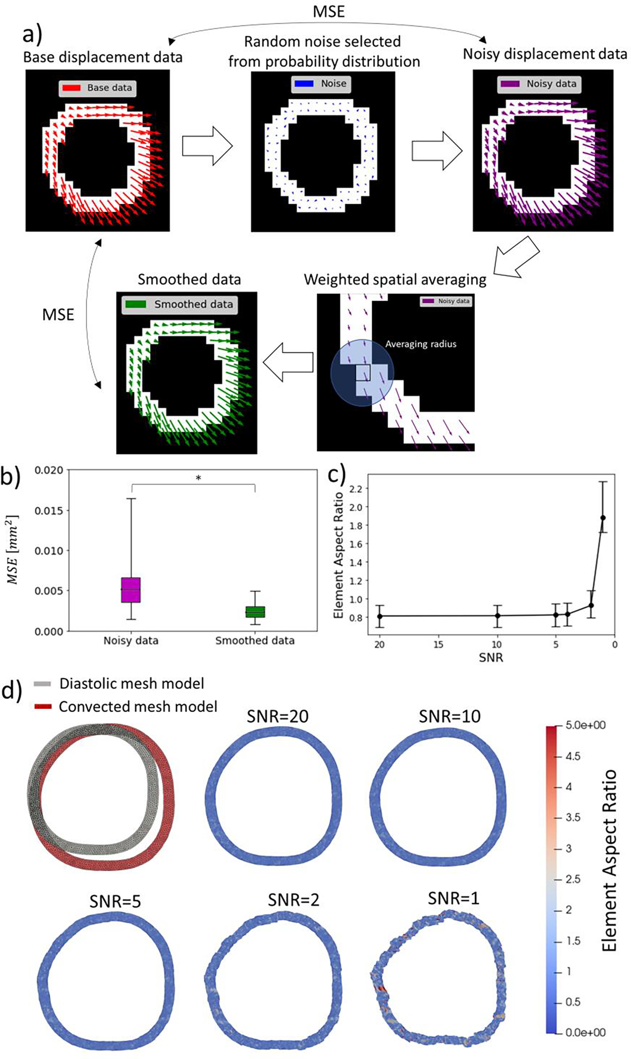
Quantification of the effect of random noise on aortic wall displacement estimations and the use of smoothing algorithms to reduce this effect. a) DENSE MRI-derived displacement distributions on segmentations of the aortic wall (or phantom) were used as base data. Random selections of background noise from the case-specific probability distribution were added to the base data to obtain a noisy displacement distribution. The mean square error (MSE) between the noisy and base data was assumed a measure of the effect of noise. A smoothing algorithm was applied to the noisy displacement distribution to reduce the effect of noise. b) The smoothing algorithm can significantly reduce the effect of noise by cutting the mean squared error by half and generating a displacement distribution that closely matches the base data. c) Effect of SNR on the quality of a convected finite element mesh using interpolated DENSE MRI measured as the aspect ratio of triangular elements. Higher levels of noise tends to distort the convected geometry generating elements with elevated aspect ratio. d) Convection of the finite element mesh of an aortic wall model at diastolic configuration into the systolic configuration with DENSE MRI-derived data with different levels of signal-to-noise ratio.

Additionally, a spatial smoothing algorithm, following the DENSE-MRI post-processing technique by Wilson et al. [10], was applied to the displacement distribution affected by noise to quantify the effectiveness of such noise reduction method. The smoothing algorithm consisted of recalculating the displacement estimation of each pixel by averaging the value of all pixels inside the segmentation within 2 pixel-widths (including the pixel of interest). To verify consistency of the result, the process was replicated for each case with a second set of random noise (Figure 9a).

2.9. Statistical analysis.

Statistics were performed with JMP^® Pro 16.0.0 (SAS Institute Inc.) and assumed a significance level of p*<0.05. Analysis of variance (ANOVA) was conducted to explore the significance of case-to-case and group-to-group (DAA, DTA, IAA, Phantom) variations. Tukey HSD test was applied for multiple comparisons, considering phase direction and group (DAA, DTA, IAA, Phantom) as independent effect variables (Table 1). Paired Student t test was applied to compare the effect of offset correction and noise reduction algorithms. The Pearson correlation coefficient $\left(r^{\mathrm{*}}\right)$ was calculated to assess correlations to time-step and 2D spatial location.

3. Results.

3.1. Identification and masking background pixels.

Calibrating the threshold value of pixel-wise standard deviation over time to define the background mask revealed that the lowest 45th percentile produced adequate background segmentations for most in vivo cases. The static masked structures included on in vivo cases included the vertebrae, left ribs, and sternum on thoracic planes, and erector spinae muscles for abdominal planes. For the in vitro studies the lowest 30th percentile was sufficient to identify the background, which consisted of the supporting blocks and portions of the water pool away and unaffected by the the moving phantom (Figure 3).

Given the similarities of the phase signal of the background for both phase-encoding directions, only plots for phase $y$ of a representative DTA in vivo case are shown (Figures 3, 4 and 5). Similar plots for representative cases of the three aortic locations and in vitro studies for both phases are included in the Supplementary material A.1.

3.2. Offset error and noise in background pixels.

The mean signals (on both enconding phases) of the background pixels was consistently found to be within the range of random noise $\left({\bar{\alpha }}_i<{\bar{\tau }}_i\right)$, and a simple single-sided Student $t$ test suggests offset errors are not significantly different than zero $(p^{\mathrm{*}}=0.7)$. The probability distribution of ${\alpha }_i(x,y)$ was approximately normal for both phases in all cases (shown in Figure 4g), with mean values consistently close to zero and an overall mean of ${\bar{\alpha }}_x=0.003\pm 0.02rad$ and ${\bar{\alpha }}_y=-0.020\pm 0.024rad$ for each phase, respectively. No significant differences in $\bar{\alpha }$ were found between any group (DAA, DTA, IAA, and phantoms). Pixel-wise offset error showed poor correlation to the pixel position $\left(r^{\mathrm{*}}<0.2\right)$ (Supplementary material A.2), meaning that offset errors, albeit small, were also not dependent on pixel position.

However, the trends observed through the best fit planes to ${\tau }_i(x,y)$ reveal that, for both phases, the noise of the signal of the background pixels increases towards the anterior direction with a slope of 0.0005 ± 0.002 rad/pixel $\left(r^{\mathrm{*}}=0.35\pm 0.16\right)$ (Figure 4f), while the average change in the lateral direction 0.00010 ± 0.00009 rad/pixel showed no consistent trend $\left(r^{\mathrm{*}}<0.1\right)$ (Supplementary material A.3). The probability distribution and mean values of ${\tau }_i(x,y)$ were similar for each encoding direction and were skewed towards zero (Figure 6c). The mean value of the pixel-wise standard deviation of phase over time $\left({\bar{\tau }}_i\right)$ was consistent among all in vivo and in vitro cases with an overall average value of ${\bar{\tau }}_x=0.062\pm 0.018\mathrm{r}\mathrm{a}\mathrm{d}$ and ${\bar{\tau }}_y=0.064\pm 0.019\mathrm{r}\mathrm{a}\mathrm{d}$ for phases $x$ and $y$, respectively (Figure 7c). No significant differences in $\bar{\tau }$ were found between any group (DAA, DTA, IAA, and phantoms) (Table 1).

Figure 6.

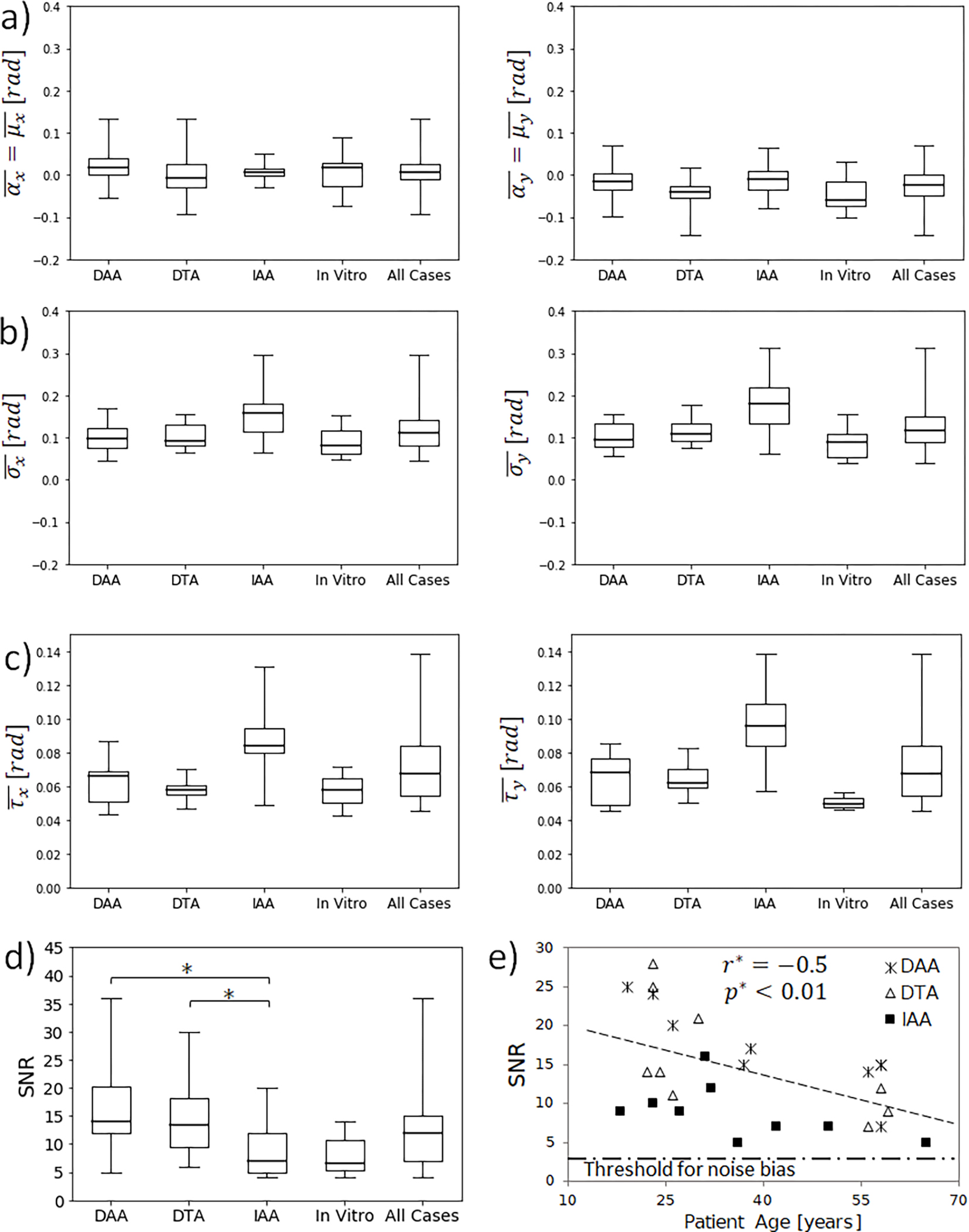
Comparisons of statistics between in vivo groups and in vitro cases. No significant differences were found for a) mean offset error $\left({\bar{\alpha }}_i\approx {\bar{\mu }}_i\right)$, b) mean of phase signal of the background standard deviation ${\bar{\sigma }}_i$, or c) mean noise (mean of standard deviation of phase data over time) ${\bar{\tau }}_i$. Left and right column show results for the phase-encoding directions x and y respectively. d) SNR was significantly larger at the thorax than at the abdomen $\left(p^{\mathrm{*}}<0.01\right)$. SNR for in vitro experiments showed no significant difference to any of the in vivo groups. e) SNR decreases with the age of volunteers due to the stiffening effect of ageing on cardiovascular tissue and impairment of cardiovascular function.

Figure 7.

a) The mean value of background signal of each time-resolved image for both motion encoding directions ${\mu }_i\left(t\right)$ remains close to zero for all in vivo and in vitro groups independent of time. b) Standard deviation of phase signal of the background of each time-resolved image ${\sigma }_i\left(t\right)$ significantly increases over time for both phase-encoding directions. Left and right column show results for the phase-encoding directions x and y respectively. Dashed line shows the least squared line fitting the ${\mu }_i\left(t\right)$ and ${\mu }_i\left(t\right)$ data from all cases.

3.3. Phase signal of background pixels and dependence over time

The phase signals of the background pixels were found to follow a normal probability distribution centered approximately at zero for both directions in all cases and all timesteps (Figure 5b). The mean value of phase signal of the background ${\mu }_i\left(t\right)$ showed no correlation to the timestep for phase $x\left(r^{\mathrm{*}}=0.05,p^{\mathrm{*}}=0.82\right)$ or phase $y\left(r^{\mathrm{*}}=\right.\left.0.35,p^{\mathrm{*}}=0.14\right)$, with overall mean values of ${\bar{\mu }}_x=0.003\pm 0.02rad$ and ${\bar{\mu }}_y=-0.020\pm 0.024rad$ respectively (Figure 7a). These mean values of phase data encode for offset displacement errors of 0.004 mm and 0.025 mm for encoding directions $x$ and $y$ respectively, which are negligible and consistent with ${\bar{\alpha }}_x$ and ${\bar{\alpha }}_y$. However, the standard deviation of phase signals of the background pixels $\sigma \left(t\right)$ showed a significant positive correlation to time for both the $x\left(r=0.81,p^{\mathrm{*}}<0.001\right)$ and $y$-directions $\left(r=0.84,p^{\mathrm{*}}<0.001\right.$), with mean values of 0.09 ± 0.02 rad and 0.10 ± 0.02 rad, and linear increments of 0.047 rad over the cardiac cycle and 0.062 rad/cycle, respectively (Figure 7 b and Supplementary Material A4). Both overall means of offset error metrics $\bar{\mu }$ and $\bar{\alpha }$ were identical, and no significant difference of $\bar{\mu }$ or $\bar{\sigma }$ was found between aortic locations or between in vivo and in vitro datasets (Figure 6a,b).

3.4. Signal to noise ratio

For the entire dataset, the average SNR was 13 ± 7. No statistical difference in SNR was found between the two phase-encoding directions, with an overall mean difference of 1.3 and $p^{\mathrm{*}}=0.45$. However, significant differences were found between aortic locations. The SNR at the DAA $\left(16.7\pm 8.5,p^{\mathrm{*}}=0.003\right)$ and DTA $\left(15.4\pm 7.6,p^{\mathrm{*}}=0.008\right.$) were significantly greater than the IAA (8.0 ± 4.1) (Figure 6d). We have also found in the in vivo datasets a correlation of decreasing SNR with volunteer age for all three aortic locations $\left(r^{\mathrm{*}}=-0.5,p^{\mathrm{*}}<0.01\right)$ (Figure 6e).

The average SNR for the in vitro experiments (8.0 ± 3.7) was not significantly different to any of the in vivo groups with $p^{\mathrm{*}}$ values of 0.06,0.13, and 1.00 for comparisons to DAA, DTA, and IAA groups, respectively. Notably, the in vitro experiment without a support block that allowed free expansion with smaller uniform displacements (Case #58 in Table 1) displayed a lower SNR than the other two experiments with support blocks that promoted the motion of the phantom upward and away from the support block (Figure 2c).

3.5. Displacement and displacement uncertainty.

The DENSE MRI-derived displacement distribution was found to strongly depend on the aortic location (Figure 1c) and in vitro configuration (Figure 2c). Detailed discussion on the different displacement patterns found at each aortic location and phantom setups are discussed elsewhere [9,16]. Averaged values of displacement magnitude are listed for each case in Table 1. Notably, the average displacement for the DAA group (1.9±0.2 mm) was significantly larger than the IAA $\left(1.2\pm 0.3\mathrm{m}\mathrm{m},p^{\mathrm{*}}=0.04\right)$. Overall, the average DENSE MRI-derived displacement uncertainty was estimated as 0.11 ± 0.10 mm.

3.6. Offset error correction.

The proposed method of subtracting the best fit offset error plane $A_i(x,y)$ from phase significantly reduced the mean offset error to a practical zero $\left({\bar{\alpha }}_i<{10}^{-10}\right)$ for all cases with negligible dispersion $\left(p^{\mathrm{*}}<0.01\right)$ (Figure 8a). The correction method also tends to reduce the mean pixel-wise standard deviation of the phase signal ${\bar{\sigma }}_i$ by 5% on average (Figure 8b), while having no effect on background noise ${\bar{\tau }}_i$.

Figure 8.

a) The offset correction method was effective in reducing the mean offset error to a practical zero for all cases and both phases. b) The offset correction method tends to decrease the phase data spread ${\bar{\sigma }}_i$ by 5% on average, with no significant effect. Left and right column show results for the phase-encoding directions x and y respectively.

3.7. Effect of noise on displacement distribution of the aortic wall.

Random selections of noise from the case-specific probability distribution induce a mean squared displacement error (MSE) of 0.006 ± 0.003 mm² (~0.07 mm of standard error) with respect to the base aortic wall displacement distribution. The application of a smoothing algorithm based on weighted spatial averaging can significantly reduce the MSE to 0.003 ± 0.002 mm² (~0.05 mm of standard error) $\left(p^{\mathrm{*}}<0.01\right)$ (Figure 9b).

4. Discussion.

4.1. Phase signal and noise on the background pixels.

The normal probability distribution of the phase signal of the background being centered near zero suggests that background noise is random with negligible fixed bias. The two metrics of mean offset error, ${\bar{\alpha }}_i$ and ${\bar{\mu }}_i$, were the result of consecutive averaging of phase signal of the background over space- and time-independent variables, with flipped consecutive spatial and temporal averaging. Given the normality of phase signal of the background, both measures were equivalent for any practical mean. Mean offset error consistently converged to values 100 -fold smaller than pixel size, with an overall average of 0.015 mm. However, the implemented correction method can further reduce the offset error to a practical zero.

The criticality of offset correction depends on the specific application of DENSE MRI. For the calculation of differential quantities, such as strain, offset errors are natually countered with the numerical differentiation process so its correction may be somewhat irrelevant. However, even small offsets can accumulate into relevant sources of error when calculating measures that rely on numerical integration methods such as the estimation of volume and volume changes [13]. The offset error obtained with the incorporated DENSE MRI scanning protocol is within the range of uncertainty, and negligible in comparison to the mean displacement of the aortic wall of healthy individuals; nevertheless, it may become relevant in the study of pathological cases.

The mean background noise was estimated at ${\bar{\tau }}_i=0.06rad$ with no significant differences between phase directions, suggesting that the noise was isotropic. The background noise consistently varied along the scan plane with a slope of approximately 0.0005±0.002 rad/pixel, incrementing in the posterior-to-anterior direction. This directional increment may be due to the uncertainty induced by involuntary respiratory motion along the supine patient’s anterior surface (Figure 6a). That is, even though the DENSE acquisition is respiration-gated, there remains a finite acceptance window on the navigator that admits some variation due to respiratory motion. Notably, the slope in values of noise of 0.0005 rad/pixel suggests that the uncertainty would vary by about 0.0075 rad around the mean value across the diameter of a typical DAA (2 cm or 15 pixels). This represents ~10% of the mean value of $\bar{\tau }$. Thus, assuming the background noise is homogeneous in the area occupied by the aortic wall may be reasonable.

The magnitude of $\bar{\tau }$ estimates the most probable variation of phase readings over time due to noise, and thus, is directly related to the concept of uncertainty. This metric provides a measure of variability relative to the mean value of the signal, and such is unaffected by the pixel-wise offset ${\alpha }_i(x,y)$ (Figure 4b). On the other hand, $\bar{\sigma }$ estimates the most probable range of signal values for the background pixels $(\bar{\mu }\approx 0)$; that is, a measure of the spread of absolute phase signals. In consequence, $\bar{\sigma }$ is affected by the added effect of temporal variability of phase ${\tau }_i(x,y)$ and by pixel-wise offset errors $\alpha (x,y)$, which is the reason for $\bar{\sigma }$ being consistently larger than $\bar{\tau }$ (Figure 6).

Though the fixed bias or directionality preference were negligible, the range of background signals increased up to 50% through the cardiac cycle (i.e., as time increased since the encoding time at the beginning of cardiac systole) (Figure 7b). Meaning that the ability to appropriately resolve the background pixels declines over the cardiac cycle, as signals from the background become comparable to those from low-moving structures. This time-dependent increase in noise signal intensity may relate to the progressive demagnetization of tissue over time, as has been described previously for other MRI techniques [18,24]. This effect may also be related to the number of cardiac cycles sampled to generate the phase data. This suggests that aortic DENSE MRI scans should be planned so as to gather the information of interest (such as e.g. systolic inflation) during the earliest time-steps of the imaging cycle. Finally, no significant differences of $\bar{\sigma }$ and $\bar{\tau }$ were found between in vivo and in vitro groups, suggesting either that the in vitro setup closely reproduced the in vivo environment or that the scanned subjects had little effect on background noise.

4.2. SNR and displacement uncertainty.

Since the background noise was consistent among individuals and groups, SNR depended primarily on the magnitude of phase signals, so as expected, SNR was greater for structures with larger displacements. SNR was calculated for each phase-encoding direction using the corresponding ROI signal and background noise. We found that SNR was generally different on each phase-encoding direction on case-to-case and group-to-group comparisons. For example, SNR for encoding direction $x(21.6\pm 1.8)$ was significantly larger than for encoding direction $y\left(11.1\pm 1.9,p^{\mathrm{*}}=0.003\right)$ for the DAA group, while SNR in $y$ direction was significantly larger (10.1 ± 0.6) than on the $x$ direction $\left(5.9\pm 0.7,p^{\mathrm{*}}=0.002\right)$ for the IAA group. These differences are related to the direction of aortic wall motion: at the DAA the aorta is displaced towards the left lung, while the IAA consistently moves towards the anterior space occupied by the peritoneal cavity (Figure 1c). For this reason, independent group-to-group comparisons of SNR by encoding directions could be misleading. Herein, we performed Tuckey HSD multiple comparisons of all SNR estimations assuming the phase encoding-direction and group-to-group variations as independent effects, and thus, comparing direction-averaged values of SNR between groups.

SNR was significantly larger in the DAA and DTA compared to the IAA, which is consistent with previous studies that have demonstrated that the thoracic aorta undergoes larger displacements during the cardiac cycle than the abdominal aorta [9,25]. Similarly, the in vitro experiments supported by blocks induced larger upward displacements and greater SNR values than the experiment with uniform expansion and smaller displacements (Figure 2c, Table 1). In addition, average SNR for in vivo cases showed a negative correlation to the volunteer age, which is likely a direct consequence of the well-known stiffening of cardiovascular tissues with age [26].

For the entire data set, the average uncertainty of DENSE MRI-derived displacement was approximately 10 -fold smaller than the pixel size (0.11 ± 0.10 mm). This supports previously published data showing that DENSE MRI is more precise and reliable than other techniques based on anatomical features/fiducial markers or pixel tracking [6,27]. The displacement uncertainty was approximately 30 -fold times smaller than the largest case-specific average displacement, and 5-fold times smaller than the lowest one, suggesting the technique is adequate to study aortic motion in this healthy patient population.

4.3. Potential Implications

Herein, we showed that random sampling of noise from the case-specific probability distribution induces a mean-squared error of 0.006 ± 0.003 mm² ~0.07 mm of standard error) on the estimated displacement distribution of the aortic wall.

Despite the small magnitude of the offset error, the background noise uncertainty can yield significant effects on DENSE-derived differential measurements such as strain estimations. Simple idealized calculations can be used to illustrate the potential impact of noise. Assuming a cylindrical vessel of 20 mm diameter, a strain of 10% will induce an increment of circumference of 6.3 mm. If this estimation of arch length change is affected by the displacement uncertainty of 0.13 mm on both ends of the arch, the estimation of strain could be affected by an error of 4% of the strain value. The potential impact rapidly increases if strain heterogeneity is to be explored with a potential error of 16% if the arch is split in four sections.

Standard noise-filtering techniques, such as temporal and spatial averaging of pixelwise displacement data, can significantly palliate the effect of noise on kinematic and dynamic analyses as long as the measurements are not biased by noise (Figure 9b) [9,25,28]. To better illustrate this effect, we interpolated DENSE MRI-derived diastolic-to-systolic displacements into finite element mesh models of the aortic wall at diastole. Then, the mesh nodes were convected with the interpolated displacement yielding a deformed systolic configuration that can be used to estimate the distribution of strain on a realistic geometry (Figure 9d) [25]. Herein, we explored how the effect of noise can dampen the use of DENSE-MRI data. It was found that DENSE MRI noise was adequately handled by the averaging effect of the node-to-node interpolation, leading to smooth systolic configurations if SNR>5 (Figure 9d). However, if the effect of noise is artificially increased (e.g. for SNR<4), the impact of noise induces distortions that render the systolic configuration completely inadequate (Figure 9c,9d).

Ageing and some cardiovascular pathologies (hypertension, atherosclerosis, aneurysms, etc) are associated with aortic stiffening, and thus, reduced aortic compliance and motion. On these cases, the relative effect of noise is potentially increased. For example, case # 27 of our dataset corresponds to a 65-year-old patient for which the SNR was the lowest value reported in this study, close to the acceptable threshold to yield unbiased results. This suggests that the application of this technique to stiffened aortas or to aortic walls with very neglible motion (such as in aneurysms), may require the use of larger magnetic field strengths to reduce the effect of noise; however, this requires further study.

5. Limitations

This retrospective study was limited to the available DENSE MRI data, most of which were performed in relatively healthy adults with mean strains greater than 4%. For applications on cardiovascular disease, the analysis of noise and uncertainty described herein should be repeated for comparison. Similarly, applications in smaller vessels or in pediatric patients should be separately evaluated given the reduced thickness of the vascular wall and potentially smaller displacements. In the future, parametric studies of the effect of encoding frequency, pixel size, number of spirals of k-space acquired, flip angle, and/or number of signal averages on the noise and uncertainty could be insightful to optimize the DENSE protocol for different aortic applications.

6. Conclusions

The analysis of background noise in 2D spiral cine DENSE MRI for healthy adult aortas suggested that the observed noise was random and isotropic, yielding negligible offset error for the encoded displacement of the descending aorta. The background noise was similar in both in vivo healthy volunteers and in vitro testing using pressurized PVA phantoms and water. However, the noise of the phase signal of the background pixels increased with time and was dependent on the spatial location in the scan plane; thus, these factors should be taken into consideration when planning DENSE MRI studies. Given an average SNR of approximately 13 and displacement uncertainty approximately one order of magnitude smaller than the pixel size and the average aortic displacement, we conclude that aortic DENSE MRI is reliable for the study of healthy adult aortas. Moreover, DENSE MRI-derived metrics can be further improved by simple offset correction algorithms and noise reduction techniques similar to 2D PC MRI velocity corrections [15]. However, noise-filtering techniques are only effective when the signal is sufficiently larger than noise, and a simple analysis presented here suggests a limit of SNR>4 is adequate for noise filtering. We recommend repeating this type of analysis in future applications of DENSE MRI for any unique vascular targets, populations, or pathologies.

Highlights.

• Signal noise increased over the elapsed scanning time and was higher in the anterior thoracic space.

• The noise was not significantly different between the three in vivo aortic locations and in vitro setups.

• SNR was significantly different at three locations along the descending aorta.

• SNR of more than 4 was acceptable to congruent strain maps.

• SNR decreased with age, falling close to the acceptable threshold on the infra-abdominal aorta of the eldest volunteer.