Quantifying the human impact of Melbourne’s 111-day hard lockdown experiment on the adult population

Abstract

Lockdown was used worldwide to mitigate the spread of severe acute respiratory syndrome coronavirus 2 and was the cornerstone non-pharmaceutical intervention of zero-COVID strategies. Many previous impact evaluations of lockdowns are unreliable because lockdowns co-occurred with severe coronavirus disease related health and financial insecurities. This was not the case in Melbourne’s 111-day lockdown, which left other Australian jurisdictions unaffected. Interrogating nationally representative longitudinal survey data and quasi-experimental variation, and controlling for multiple hypothesis testing, we found that lockdown had some statistically significant, albeit small, impacts on several domains of human life. Women had lower mental health (−0.10 s.d., P = 0.043, 95% confidence interval (CI) = −0.21 to −0) and working hours (−0.13 s.d., P = 0.006, 95% CI = −0.22 to −0.04) but exercised more often (0.28 s.d., P < 0.001, 95% CI = 0.18 to 0.39) and received more government transfers (0.12 s.d., P = 0.048, 95% CI = 0.001 to 0.24). Men felt less part of their community (−0.20 s.d., P < 0.001, 95% CI = −0.30 to −0.10) and reduced working hours (−0.12 s.d., P = 0.004, 95% CI = −0.20 to −0.04). Heterogeneity analyses demonstrated that families with children were driving the negative results. Mothers had lower mental health (−0.27 s.d., P = 0.014, 95% CI = −0.48 to −0.06), despite feeling safer (0.26 s.d., P = 0.008, 95% CI = 0.07 to 0.46). Fathers increased their alcohol consumption (0.35 s.d., P = 0.002, 95% CI = 0.13 to 0.57). Some outcomes worsened with lockdown length for mothers. We discuss potential explanations for why parents were adversely affected by lockdown.

Of all the non-pharmaceutical interventions introduced to mitigate the spread of severe acute respiratory syndrome coronavirus 2 (coronavirus disease 2019 (COVID-19)), none has been so ‘intrusive’ and ‘drastic’ as the lockdown¹. It is commonly understood as a restriction of the individual right to move freely that ‘applies to all people’, albeit some categorization systems label such mobility restrictions as ‘partial lockdown’, ‘household confinement’ or ‘movements for non-essential activities forbidden’². By the end of April 2020, half of humanity was in some form of lockdown: almost 4 billion people across 90 countries were asked by their governments to stay at home³. By the end of 2021, some countries had ordered their residents into their eighth lockdown, while other places had experienced over 100 days sheltered in place.

Early on in the pandemic, stay-at-home orders with all their obvious personal costs were accepted as an essential strategy to set up pandemic response systems and to prevent health services from being overwhelmed^4,5. During the second wave in 2020, however, an international scientific debate erupted⁶ over whether community spread could only be controlled through maximum suppression, which would have required hard lockdowns and border closures (zero-COVID strategy)^7,8, or whether less restrictive mitigation measures would achieve the same goal⁹. Evidence exists both in favour of elimination strategies to achieve their primary objective^10–13 and against them^14–16, while some proposed that less intrusive non-pharmaceutical interventions may be more appropriate should infection numbers surge¹.

However, zero-COVID strategies cannot be used indefinitely because lockdown requires many sacrifices from residents¹⁷. Such sacrifices include poorer mental health^18–20, increases in loneliness because of social isolation^21–24, and the abandonment of healthy, or adoption of unhealthy, behaviours to cope with that isolation. Importantly, a great concern was that lockdowns exacerbated social, economic and sex inequalities^24–28, harming in particular women^29,30, families³¹, and individuals from a lower socio-economic background³². The burden of lockdown to mothers was at the forefront of the popular debate, with some descriptive studies showing that the well-being of mothers was likely to be most impaired^30,33–35. The closure of schools or childcare centres meant that children had to be cared for and taught at home. Women were expected to cover such homeschooling and caring duties^36,37. The impact of both the pandemic and lockdowns on mothers’ labour supply were deemed substantial^37–40.

Although studies identified the causal impact of lockdown, mostly on mental health^29,32, most studies that have been produced since the onset of lockdowns have relied on before–after comparisons¹⁸, without addressing the many confounding factors that accompany lockdowns. The problem is that lockdowns were not imposed exogenously. In many jurisdictions, including the UK, the USA and some European countries, lockdown was a last-resort policy measure that occurred after a string of events, with the aim of flattening the curve of exponentially growing caseloads, patients in intensive care units and number of deaths from COVID-19. Thus, lockdown impact estimates may be overshadowed by COVID-related trends of increasing morbidity and mortality. Lockdowns also caused severe economic contraction, job loss and business closures at the macroeconomic level. Thus, lockdown impact estimates may be confounded by income shocks that threatened the financial sustainability of households. In both cases, lockdown impact estimates are probably severely overestimated.

In this study, we used methods from the economic policy evaluation literature (difference-in-differences models) in combination with high-quality, nationally representative longitudinal data (Household, Income and Labour Dynamics in Australia (HILDA) Survey) to overcome these identification issues. We studied the natural experiment that arose from Australia’s second 2020 lockdown. On 9 July 2020, Australia’s second largest city, Melbourne, the capital of the state of Victoria, was locked down for 111 consecutive days using an aggressive zero-COVID strategy to return to zero infections^41,42, while other Australian jurisdictions remained open. The Melbourne case is of scientific importance. Melbourne endured the second-longest consecutive hard lockdown in 2020 (after Buenos Aires) and held the unenviable record of the greatest cumulative time spent in COVID-19 lockdown worldwide by mid-2022. Melbourne’s zero-COVID achievement after a hard and long lockdown was being hailed by the scientific community⁴³.

Melbourne’s natural experiment is also of methodological value because it generated a valid control group (that is, Sydneysiders) against which changes in the lives of Melbournians could be compared against. While at least two other studies exist that use similar methods for evaluating shorter lockdown effects on adults in the USA²⁹ and the UK³² on mental health, our study evaluates the causal impact of Melbourne’s hard and long lockdown on a range of life’s facets for adults. The breadth and quality of our large data allowed us to comprehensively interrogate the unequal impacts of lockdown across multiple domains, including health, health behaviours, feelings of social connectedness, labour supply and income, and study the dose–response to lockdown.

Results

The natural experiment of the Melbourne lockdown

Melbourne’s lockdown occurred two months after a successful national lockdown (23 March–15 May 2020), when life in Australia was returning to normality. Australia-wide, new daily infections in early June 2020 numbered fewer than 20, school students had returned to the classroom, workers were permitted to return to the office and service industries were allowed to operate again, albeit with capacity limits. In late June, breaches in the hotel quarantine system saw case numbers in Melbourne begin to rise again. This led to the reimposition of stay-at-home orders in certain postcodes in the western and northern suburbs of Melbourne on 2 July before being extended to all areas, as well as one shire on the outskirts of Melbourne, on 9 July. Borders closed between New South Wales, the most populous state in Australia, and Victoria on the same day. On 2 August, the Victorian Government declared a state of disaster and imposed an 20:00 to 5:00 curfew on Melbournians and stay-at-home orders on regional Victorians. Stay-at-home orders remained in place in Melbourne until 28 October but were lifted earlier (on 17 September) in regional Victoria.

Although lockdown occurred both in Melbourne and regional Victoria, we focused on the Melbourne case only. With international and state borders closed, and travel-distance restrictions in place within Victoria, Melbournian residents could not easily escape lockdown measures. Compliance with lockdown orders was relatively high in Melbourne, in contrast to the rest of Victoria (Methods).

In contrast to many other international experiences, the Melbourne lockdown occurred in the absence of both widespread household financial difficulties and public health challenges. Like many other advanced economies (for example, New Zealand, Germany and Singapore), households and businesses were spared severe financial difficulty due to the immediate availability of generous federal fiscal stimulus programmes that buffered businesses’ profit loss, while keeping workers employed with compensated pay (the JobKeeper programme), and which paid a substantial supplement to the incomes of those relying on income support payments. But where the Melbourne lockdown differed was that it commenced when daily new infections were relatively low (<100). Even during lockdown, the maximum number of new daily infections peaked at 725 (Fig. 1). The number of deaths that subsequently occurred during lockdown were concentrated among those aged 70 years or older, with 75% occurring in residential care. Thus, cases did not cause a health burden of disease among young people, the working age or younger retiree populations that were most affected in their daily activities by lockdown.

Fig. 1 |. Description of the natural experiment with a timeline of COVID-19 daily infection numbers, lockdown dates and HILDA Survey data collection windows.

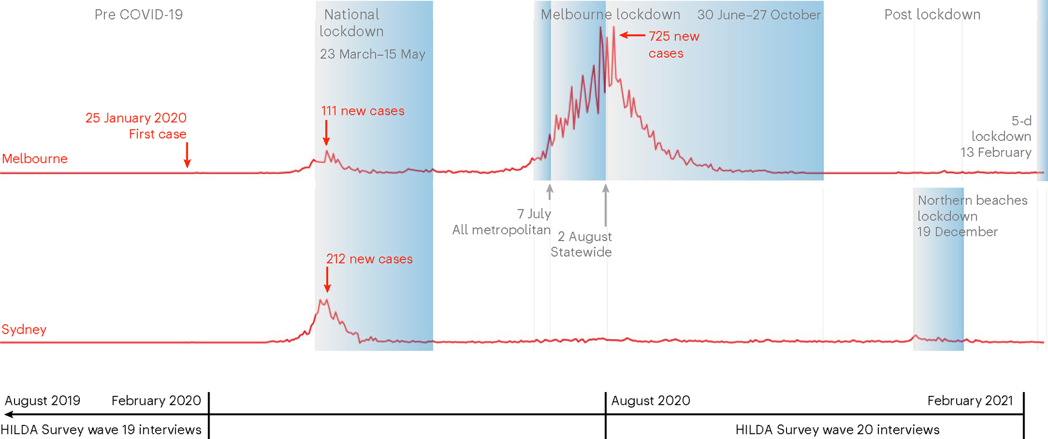
The figure was prepared by the authors based on data available from Our-World-in Data. HILDA Survey waves are collected annually between August and February the following year. A small number of individuals are interviewed in March. For information on the lockdown rollout, and data collection, protocol and composition, see Methods.

Meanwhile, in the rest of the country, including Sydney, Australia’s largest city and the capital of New South Wales, residents could move freely. Most businesses were allowed to operate, including in the hospitality sector, albeit with some capacity or density limits. The only exception was a 5-day mobility restriction in one out of 30 government areas in the Greater Sydney area in mid-December 2020, and even that did not involve a stay-at-home order.

Fortuitously, during Melbourne’s lockdown period, the 20th wave of Australia’s nationally representative HILDA Survey was undertaken (Fig. 1). This household panel commenced in 2001 with a nationally representative sample of Australian households (Methods). In line with data collection protocols in previous years, almost all 2020 HILDA Survey participants (>93%) were interviewed between August and late October, which fell directly within the window of Melbourne’s lockdown experiment.

We compared the outcomes in Melbourne with the outcomes in Sydney, the most comparable city to Melbourne, which was not locked down. In the HILDA Survey there were 9,441 individuals (n) who either lived in Sydney or Melbourne between 2011 and 2020, which left us with 60,108 person-years of observations (PYO).

For the analysis, we derived proxies that captured comprehensively and broadly adult human life across four domains. For each domain, we identified three standard measures that have consistently been measured annually over the past 10 years and which referred in each wave to the current time period (Methods and Supplementary Table 1 for definitions): (1) health: mental health (0–100), general health (0–100) and bodily pain (0–100); (2) health behaviours: body mass index (BMI) (kg m⁻²), frequency of physical activity (from never (1) to every day (6)), and frequency of alcohol consumption (from never (1) to every day (7)); (3) perceptions of social connectedness: safety (from very dissatisfied (0) to very satisfied (10)), loneliness (from strongly disagree (1) to strongly agree (7)) and feeling part of the local community (from very dissatisfied (0) to very satisfied (10)); (4) labour supply and income (weekly): working hours (including 0), salary and wages from all jobs, and government transfers excluding family benefits (both in Australian dollars). Time variation in these outcomes for both the Melbourne and Sydney samples are reported in Supplementary Figs. 1 and 2.

Sample sizes differed for each outcome but ranged between 45,053 PYO (n = 8,027) and 59,236 PYO (n = 9,329) (Supplementary Fig. 3). In addition, we analysed three outcomes collected in a 2020 COVID-19 module (n = 5,713), which asked about individuals’ past COVID-19 experience (positive test = 1, otherwise = 0) and self-assessed risk of both infection and serious illness if infected (both scaled between 0% and 100%).

The causal impact of lockdown

Many dimensions of human life significantly changed for Melbournians in 2020 when compared against the long-term average (2011–2019) (Table 1), in both positive and negative ways. A simple before and during lockdown comparison of outcomes for Melbournians could disguise the possibility that outcome changes were caused by Australia’s first and nationwide lockdown, which would have also affected individuals in other jurisdictions, or other unobservable factors, such as the existential threat of a global pandemic or international travel restrictions.

Table 1|.

Summary statistics and definitions, separated according to treatment (Melbourne) and control (Sydney) group, before and during lockdown

Variables (ranges)	Melbourne (2011–2019)			Melbourne (2020)			Test (1)=(2)			Sydney (2011–2019)			Sydney (2020)			Test(3)=(4)
	(1)			(2)			P	95% CI		(3)			(4)			P	95% CI
	Observed	Mean	s.d.	Observed	Mean	s.d.		Lower bound	Upper bound	Observed	Mean	s.d.	Observed	Mean	s.d.		Lower bound	Upper bound
PanelA: health
Mental health (0–100)	24,398	72.55	17.7	2,772	68.65	18.66	0	−4.81	−2.99	22,697	72.51	17.49	2,344	70.6	18.23	0.001	−3.07	−0.75
General health (0–100)	24,208	68.47	20.4	2,758	67.95	19.72	0.29	−1.48	0.44	22,513	67.99	20.38	2,335	67.14	20.22	0.239	−2.27	0.57
Bodily pain (0–100)	24,332	74.03	23.69	2,770	74	23.21	0.963	−1.19	1.13	22,715	74.35	23.87	2,344	73.77	23.44	0.458	−2.09	0.94
Panel B: health behaviours
BMI (10.4–76.7)	23,420	26.5	5.6	2,722	27.15	6.31	0	0.35	0.96	21,757	25.66	5.22	2,289	26.09	5.41	0.008	0.11	0.75
Frequency of alcohol consumption (1–7)	21,802	3.41	1.6	2,499	3.43	1.67	0.668	−0.06	0.1	18,786	3.4	1.68	1,966	3.39	1.67	0.833	−0.12	0.09
Frequency of physical activity (1–6)	24,389	3.57	1.53	2,770	3.77	1.57	0	0.12	0.27	22,700	3.44	1.57	2,344	3.51	1.58	0.247	−0.05	0.18
Panel C: social connectedness
Feeling safe (0–10)	27,427	8.18	1.55	3,015	8.31	1.56	0.002	0.05	0.2	26,140	8.09	1.61	2,603	8.22	1.51	0.005	0.04	0.23
Feeling lonely (1–7)	24,247	2.64	1.77	2,760	2.73	1.77	0.057	0	0.17	22,603	2.74	1.74	2,326	2.72	1.7	0.576	−0.13	0.07
Feeling part of the local community (0–10)	27,386	6.7	2.11	3,012	6.65	2.2	0.275	−0.16	0.05	26,094	6.69	2.05	2,602	7	1.98	0	0.19	0.42
Panel D: labour supply and income
Working hours (0–168)	27,445	23.93	20.18	3,017	20.27	20.07	0	−4.58	−2.74	26,170	23.71	21.07	2,604	23.78	20.37	0.912	−1.19	1.33
Weekly income (0–16,561)	27,445	707.6	874.4	3,017	725.5	927.4	0.392	−23.14	58.96	26,170	717.7	909.7	2,604	788.4	916.2	0.005	21.08	120.3
Weekly government transfer (0–5,211)	27,445	56.65	125.3	3,017	84.48	174.3	0	20.2	35.47	26,170	61.57	132.8	2,604	84.14	190.1	0.008	5.84	39.3
Panel E: demographics
Age (15–98)		43.51	18.06		44.04	18.39	0.215	−0.31	1.37		42.9	18.32		44.07	18.38	0.025	0.14	2.19
Partnered (0–1)		0.6	0.49		0.61	0.49	0.41	−0.01	0.03		0.6	0.49		0.59	0.49	0.971	−0.03	0.03
Number of adults (0–9)		2.65	1.17		2.66	1.12	0.805	−0.05	0.06		2.78	1.29		2.74	1.29	0.42	−0.14	0.06
Number of kids (0–8)		0.78	1.06		0.76	1.04	0.426	−0.07	0.03		0.75	1.08		0.76	1.06	0.782	−0.06	0.08
Percentage who graduated from university (0–1)		0.33	0.47		0.35	0.48	0.094	0	0.04		0.37	0.48		0.41	0.49	0.06	0	0.07

See Supplementary Table 1 for the definition, scaling and transformation of outcome variables. P values were computed from two-sided t-tests; thus, they are equal to each other.

For this reason, we compared outcomes for individuals before and during Melbourne’s lockdown with individuals who resided in Sydney. To adjust for the remaining differences between Melbourne and Sydney, we estimated a difference-in-differences econometric model (Methods). In this model, we controlled for city-level differences and city-specific non-linear time trends in outcomes to allow for differential time trends pre-lockdown, factors that may have changed over time for individuals (age group, marital status, highest level of education, number of adults and number of children younger than 25 in the household), individual-specific fixed effects, and mode and month of the interview, which changed slightly in 2020 (Supplementary Fig. 4). The models were estimated separately for women and men because previous literature emphasized the differential effects of both pandemic and lockdowns according to sex^30–40.

To make the estimates representative for the Australian population, survey component-specific sample weights were applied in each regression. Standard errors were clustered at the household level to adjust for repeated observations within households. All estimates were expressed in terms of s.d. away from the standardized zero mean (beta coefficients labelled as β) to facilitate comparisons of treatment effect sizes.

The model yields a causal estimate of lockdown under the assumption that outcomes in Melbourne and Sydney would have had the same trend in the absence of lockdown. It is common in the literature to test this assumption within an event-study framework, which presents estimated treatment effects before and after policy implementation. We demonstrated that there were no relevant anticipation effects in the years before policy implementation (2011–2019) (Supplementary Fig. 5). Differential pre-lockdown trends could be rejected for most outcome measures (Supplementary Table 2). We demonstrated that none of the few statistically significant differential trends would invalidate our findings in any domain.

This econometric model revealed that, on average, lockdown had statistically significant albeit small impacts on several domains of human life (Fig. 2 and Supplementary Tables 4 and 5, full results). Regarding the health domain, lockdown led to a statistically significant but small decline in mental health for women (β = −0.11 s.d., P = 0.043, 95% confidence interval (CI) = −0.21 to −0.00). For men, the decline was not statistically significant (β = −0.09 s.d., P = 0.087, 95% CI = −0.20 to 0.01). No statistically significant effects were found for general health or bodily pain.

Fig. 2 |. Lockdown treatment effects (expressed in s.d.), separately for men and women.

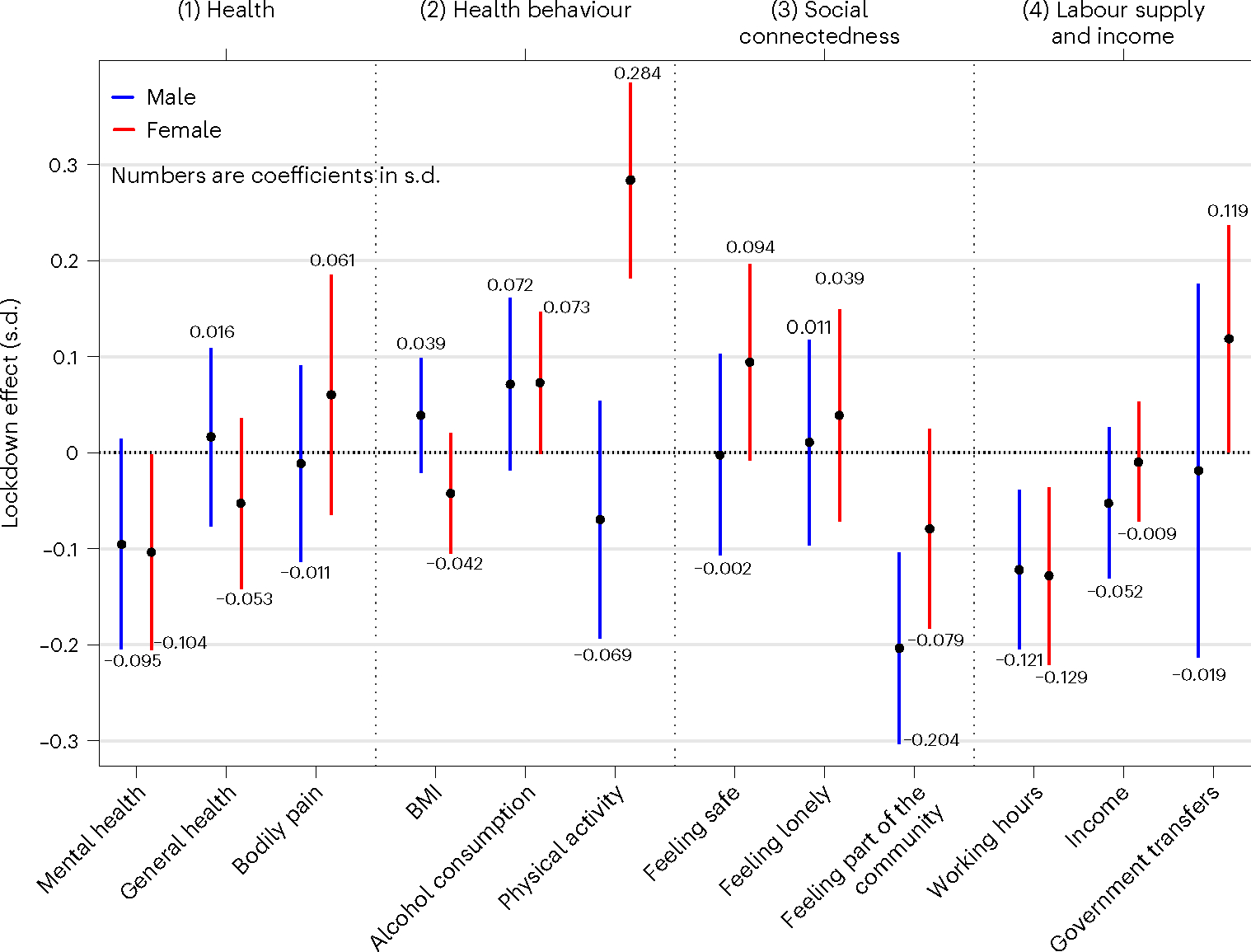
Estimated treatment effects and their 95% CIs. Each estimate was obtained from separate difference-in-differences regressions of a specific outcome, estimated separately for men (blue) and women (red). Treatment effects are interpreted as outcome changes in Melbourne between 2019 and 2020 relative to outcome changes in Sydney between 2019 and 2020, holding constant location fixed effects, location-specific time trends (wave year indicators interacting with Melbourne indicators), individual-specific effects and time-varying observable confounders. Each regression applies sample weights to make the sample representative of the population (Methods, equation (1)). Human impact is measured across four domains of human life: (1) health (mental health, n = 24,357 for male and 27,854 for female), general health (n = 24,192 for male and 27,622 for female) and bodily pain (n = 24,336 for male and 27,825 for female); (2) health behaviours (BMI, n = 23,622 for male and 26,566 for female), frequency of alcohol consumption (n = 21,731 for male and 23,322 for female) and frequency of physical activity (n = 24,355 for male and 27,848 for female); (3) social connectedness (feeling safe, n = 27,939 for male and 31,246 for female), feeling lonely (n = 24,237 for male and 27,699 for female) and feeling part of the local community (n = 27,907 for male and 31,187 for female); (4) labour supply and income (weekly working hours (n = 27,964 for male and 31,272 for female), weekly income from all sources (n = 27,964 for male and 31,272 for female) and weekly government transfers excluding family benefits (n = 27,964 for male and 31,272 for female) (see Supplementary Table 1 for definitions). Each outcome is standardized to mean = 0 and s.d. = 1. Standard errors are clustered at the household level to account for the fact that all household members (aged 15 or older) were interviewed and that full households were mobility-restricted in the same location. Supplementary Tables 4 and 5 present the full model results.

Regarding the health behaviour domain, lockdown had no statistically significant effects on BMI (for women: β = −0.04 s.d., P = 0.201, 95% CI = −0.10 to 0.02; for men: β = −0.04 s.d., P = 0.206, 95% CI = −0.02 to 0.010) or alcohol consumption (for men: β = 0.07 s.d., P = 0.120, 95% CI = −0.02 to 0.16; for women: β = 0.07 s.d., P = 0.054, 95% CI = −0.00 to 0.15). However, the lockdown statistically significantly increased the frequency of physical activity for women (β = 0.28 s.d., P < 0.001, 95% CI = 0.18 to 0.39).

In the social connectedness domain, lockdown statistically significantly reduced feelings of being part of the local community for men (β = −0.20 s.d., P < 0.001, 95% CI = −0.30 to −0.10). Regarding the labour supply and income domain, we found no statistically significant effect of lockdown on current salaries and wages or government transfers; however, it statistically significantly reduced working hours by 0.12 s.d. for men (P = 0.004, 95% CI = −0.20 to −0.04) and by 0.13 s.d. for women (P = 0.006, 95% CI = −0.22 to −0.04).

Formal testing of differences in treatment effects between men and women (Supplementary Table 6) showed statistically significant differences in the health behaviour domain (physical exercise, Δ = 0.35, P < 0.001, 95% CI = 0.19 to 0.52; BMI, Δ = −0.08, P = 0.050, 95% CI = −0.16 to 0). Sex differences in the treatment effects reported in the health, social connectedness and labour supply and income domains were not statistically significant, in particular for mental health (Δ = −0.01, P = 0.903, 95% CI = −0.15 to 0.13) and hours worked (Δ = −0.01, P = 0.907, 95% CI = −0.13 to 0.12) for which treatment effect sizes were comparable between men and women. The null hypothesis for differences in the social connectedness domain, where treatment effect sizes were remarkably different between men and women, could not be rejected, albeit at a greater risk of making a type II error with P values close to but strictly greater than 0.05 (for example, feeling part of the local community, P = 0.062).

Formal testing suggests that the common trend assumption was rejected for men for the outcome of feeling part of the local community (P = 0.011) (Supplementary Table 2). However, the hypothesis was rejected because of two outlier differences, where the outcome was more statistically significant in Melbourne than Sydney in the years 2011 and 2015. Otherwise, the two lines were perfectly overlapping in the pretreatment period between Melbourne and Sydney. A test for equal trends for physical exercise frequency for women could not be rejected (P = 0.101).

To ensure that our results were not a statistical artefact, we conducted a series of robustness checks that are recommended when dealing with many outcome measures per domain (multiple hypothesis testing (MHT) adjustment) and using difference-in-differences models. MHT adjustments within each domain demonstrate that all statistically significant treatment effects are statistically significant at the 5% level or better for both women and men (Supplementary Table 7).

Further robustness checks showed that the treatment effects were not produced by the 251 survey respondents who were interviewed outside the lockdown period (Supplementary Fig. 6), nor by the choice of control group (Supplementary Fig. 7, which used Adelaide, Brisbane and Perth as the control group). Placebo tests, in which we used Sydney as treatment group and the cities of Adelaide, Brisbane and Perth as the control group, revealed absence of any treatment effect (Supplementary Fig. 8).

Inequalities in the lockdown effect

Lockdown had statistically significant impacts on the average population, but treatment effects were mostly small in magnitude (β < 0.2 s.d.). It is possible, however, that average effects by sex disguised harm to specific groups of the population. As much of the discourse has focused on the inequality of the burden of lockdown^20,24–34, we explored heterogeneity in the treatment effect by policy-relevant subgroups and exposure length to lockdown. The policy-relevant subgroups (Supplementary Table 3) were: (1) whether the household had young children (a proxy for time pressure on and overwork for carers); (2) whether the respondent lived alone (a proxy for lack of social interaction and loneliness); (3) whether the respondent had a mental health problem in the previous year (a proxy for health care needs and frailty); (4) whether the household ranked below the median household income (a proxy for poverty); and (5) whether the respondent lived in an apartment or semidetached house (a proxy for potential overcrowding). These subgroups were not mutually exclusive as some individuals belonged to several groups.

This exploratory analysis revealed that most statistically significant and sizeable treatment effects across all groups and domains were found for mothers—women with children younger than 15 years (Fig. 3)—while for all other groups we could only find at best two statistically significant treatment effects. Mothers experienced statistically significant and medium-sized declines in the health domain (mental health: β = −0.27 s.d., P = 0.014, 95% CI = −0.48 to −0.06; general health: β = −0.22 s.d., P = 0.032, 95% CI = −0.43 to −0.02) and medium-sized increases in the social connectedness domain (feelings of loneliness: β = 0.28 s.d., P = 0.018, 95% CI = 0.05 to 0.51). These negative effects occurred despite improvements on other dimensions captured in the social connectedness domain (feelings of safety: β = 0.26 s.d., P = 0.008, 95% CI = 0.07 to 0.46) and the health behaviour domain (frequency of physical activity: β = 0.28 s.d., P = 0.016, 95% CI = 0.05 to 0.51). Mothers were negatively affected in the labour supply and income domain only through reductions in their working hours, which decreased by 0.22 s.d. (P = 0.022, 95% CI = −0.41 to −0.03). Treatment effects for mothers were significantly different from the treatment effects estimated for women without dependent children, with two exceptions. The hypothesis of equality of treatment effects could not be rejected for physical activity frequency (P = 0.669) and working hours (P = 0.176). For these two outcomes, treatment effects were also of similar effect size across the two groups (Table 2).

Fig. 3 |. Lockdown treatment effects (expressed in s.d.), separately for men and women within socially relevant subgroups.

Estimates (and 95% CIs) obtained from separate difference-in-differences regressions of a specific outcome on the treatment group indicator. a, Mental health. b, General health. c, Bodily pain. d, BMI. e, Frequency of alcohol consumption. f, Frequency of physical activity. g, Feeling safe. h, Feeling lonely. i, Feeling part of the local community. j, Working hours. k, Weekly income. l, Government income support. Treatment effect is interpreted as s.d. differences from the mean outcome (standardized to 0). See Fig. 2 for details of the model specification. See Supplementary Tables 1 and 3 for variable definitions in each domain (1–4) and the five subgroup definitions (with young child, lone individual, had low mental health in 2019, bottom income below the median and lives in an apartment). Each panel presents the results for a different outcome. Sample sizes for each estimate are reported in Supplementary Table 15. Supplementary Tables 17–21 present the full model results.

Table 2|.

Estimated treatment effects for each vulnerable group and its counterfactual in the female sample

Domain		Young child			Lonely			Low mental health			Low income			Living in an apartment
		Yes	No	P	Yes	No	P	Yes	No	P	Yes	No	P	Yes	No	P
(1) Health outcomes	Mental	−0.268 (0.108)	−0.040 (0.059)	0.072	−0.082 (0.105)	−0.107 (0.056)	0.836	−0.088 (0.129)	−0.126 (0.054)	0.783	−0.072 (0.073)	−0.146 (0.070)	0.469	−0.217 (0.098)	−0.059 (0.059)	0.171
	General	−0.224 (0.104)	0.018 (0.047)	0.030	0.008 (0.087)	−0.059 (0.049)	0.501	−0.262 (0.105)	−0.029 (0.054)	0.042	−0.082 (0.063)	−0.014 (0.057)	0.412	−0.031 (0.079)	−0.078 (0.051)	0.613
	Bodily pain	0.035 (0.149)	0.084 (0.067)	0.576	0.255 (0.115)	0.036 (0.068)	0.099	0.105 (0.124)	0.050 (0.054)	0.693	0.113 (0.098)	0.013 (0.068)	0.394	0.157 (0.126)	0.024 (0.067)	0.351
(2) Health behaviour	BMI	0.064 (0.054)	−0.080 (0.037)	0.036	−0.169 (0.058)	−0.023 (0.035)	0.033	−0.153 (0.114)	−0.020 (0.031)	0.254	−0.041 (0.052)	−0.032 (0.033)	0.883	−0.081 (0.058)	−0.027 (0.037)	0.435
	Frequency of alcohol consumption	0.128 (0.078)	0.023 (0.041)	0.114	−0.160 (0.117)	0.104 (0.037)	0.031	0.021 (0.107)	0.082 (0.038)	0.585	0.038 (0.050)	0.110 (0.050)	0.311	0.017 (0.074)	0.090 (0.040)	0.384
	Frequency of physical activity	0.282 (0.117)	0.266 (0.059)	0.699	0.260 (0.139)	0.287 (0.054)	0.858	0.122 (0.138)	0.307 (0.055)	0.214	0.262 (0.075)	0.309 (0.068)	0.648	0.357 (0.105)	0.249 (0.059)	0.373
(3) Social connection	Feeling safe	0.265 (0.099)	0.012 (0.063)	0.013	0.007 (0.136)	0.107 (0.055)	0.497	0.269 (0.163)	0.067 (0.053)	0.232	0.095 (0.073)	0.092 (0.074)	0.982	0.181 (0.103)	0.054 (0.057)	0.283
	Feeling lonely	0.281 (0.119)	−0.057 (0.061)	0.016	0.141 (0.132)	0.014 (0.059)	0.380	−0.032 (0.157)	0.051 (0.058)	0.616	0.051 (0.085)	0.015 (0.066)	0.737	0.087 (0.104)	−0.001 (0.065)	0.475
	Feeling part of the local community	0.007 (0.108)	−0.118 (0.060)	0.207	−0.017 (0.121)	−0.093 (0.057)	0.567	0.111 (0.142)	−0.109 (0.055)	0.144	−0.146 (0.082)	−0.011 (0.064)	0.197	0.108 (0.098)	−0.165 (0.061)	0.018
(4) Labour supplyand income	Working hours	−0.222 (0.098)	−0.084 (0.046)	0.176	−0.057 (0.152)	−0.143 (0.046)	0.585	−0.058 (0.088)	−0.138 (0.050)	0.421	−0.171 (0.064)	−0.078 (0.063)	0.296	−0.101 (0.100)	−0.134 (0.041)	0.758
	Income	0.000 (0.065)	−0.008 (0.034)	0.870	0.078 (0.105)	−0.021 (0.030)	0.364	−0.000 (0.062)	−0.009	0.893	−0.041 (0.032)	0.031 (0.053)	0.245	−0.000 (0.064)	−0.019 (0.031)	0.785
	Government income	0.090 (0.104)	0.066 (0.057)	0.365	0.165 (0.092)	0.119 (0.065)	0.679	0.176 (0.124)	0.119 (0.064)	0.672	0.152 (0.079)	0.066 (0.078)	0.440	0.025 (0.124)	0.146 (0.056)	0.367

The table reports the estimates of treatment for each outcome and subgroup. Clustered standard errors are shown in parentheses. The third column reports the P value associated with the two-sided t-tests of equality of treatments across two mutually exclusive subgroups.

The conclusions for mothers were somewhat sensitive to adjusting the P values for MHT. Adjustments were made for 15 hypotheses that were tested across five vulnerable groups and three outcomes per domain (Supplementary Table 8). Treatment effects were statistically significant at the 5% level or better for mental health (P = 0.039) and feelings of safety (P = 0.029), but were no longer statistically significant at strict significance levels of 5% or better for general health (P = 0.079), frequency of physical activity (P = 0.099) and feelings of loneliness (P = 0.059). The effect of lockdown on working hours was no longer statistically significant at any conventional significance level (P = 0.217). With the exception of feelings of safety (P = 0.028), we found no significantly different pretreatment trends (Supplementary Table 2). However, for feelings of safety, this was exclusively driven by differential trends that occurred in 2011 and 2012, while trends were the same since 2016 (Supplementary Fig. 5).

For fathers, the only statistically significant impact was found in the health behaviour domain. Fathers significantly increased their frequency of alcohol consumption by 0.35 s.d. (P = 0.002, 95% CI = 0.13 to 0.57), a medium-sized effect that differed significantly from the treatment effect estimated for men without young children (Δ = 0.37 s.d., P = 0.002, CI = 0.13 to 0.60; Table 3). The treatment effect was robust to adjustments for MHT (P = 0.010; Supplementary Table 9) and there were no significant pretreatment trends for this outcome (P = 0.283; Supplementary Table 2).

Table 3|.

Estimated treatment effects for each vulnerable group and its counterfactual in the male sample

Domain		With young child			Feeling lonely			Low mental health			Low income			Living in an apartment
		Yes	No	P	Yes	No	P	Yes	No	P	Yes	No	P	Yes	No	P
(1) Health outcomes	Mental health	−0.148 (0.131)	−0.071 (0.058)	0.729	−0.109 (0.123)	−0.093 (0.060)	0.906	−0.134 (0.189)	−0.064 (0.051)	0.713	−0.071 (0.085)	−0.104 (0.071)	0.769	−0.095 (0.116)	−0.077 (0.061)	0.889
	General health	−0.036 (0.095)	0.043 (0.051)	0.328	0.062 (0.097)	0.011 (0.050)	0.648	−0.003 (0.135)	0.026 (0.048)	0.838	0.017 (0.060)	0.005 (0.065)	0.888	0.038 (0.091)	−0.009 (0.048)	0.644
	Bodily pain	−0.121 (0.105)	0.027 (0.061)	0.271	0.036 (0.106)	−0.026 (0.055)	0.604	0.185 (0.157)	−0.032 (0.054)	0.188	−0.131 (0.078)	0.094 (0.071)	0.039	−0.013 (0.101)	−0.040 (0.054)	0.816
(2) Health behaviour	BMI	0.039 (0.064)	0.032 (0.034)	0.799	0.091 (0.077)	0.031 (0.032)	0.470	−0.004 (0.090)	0.042 (0.032)	0.627	0.086 (0.050)	−0.012 (0.032)	0.098	0.010 (0.042)	0.038 (0.037)	0.614
	Frequency of alcohol consumption	0.351 (0.113)	−0.027 (0.048)	0.002	−0.006 (0.103)	0.086 (0.049)	0.415	0.098 (0.150)	0.071 (0.046)	0.862	0.093 (0.076)	0.056 (0.053)	0.694	0.211 (0.083)	0.025 (0.053)	0.059
	Frequency of physical activity	−0.073	−0.036 (0.131)	0.687 (0.070)	0.045	−0.072 (0.131)	0.424 (0.068)	−0.076	−0.057 (0.176)	0.916 (0.064)	−0.223	0.090 (0.096)	0.010 (0.075)	−0.158	−0.028 (0.119)	0.357
(3) Social connectedness	Feeling safe	−0.018 (0.100)	−0.005 (0.061)	0.976	0.104 (0.112)	−0.015 (0.057)	0.347	−0.015 (0.242)	0.011 (0.050)	0.914	−0.050 (0.088)	0.035 (0.057)	0.417	0.058 (0.092)	−0.035 (0.064)	0.405
	Feeling lonely	0.127 (0.110)	−0.040 (0.068)	0.151	−0.036 (0.160)	0.024 (0.055)	0.721	0.039 (0.211)	0.007 (0.054)	0.883	0.044 (0.082)	−0.012 (0.067)	0.596	0.019 (0.110)	0.016 (0.058)	0.978
	Feeling part of the local community	−0.080 (0.088)	−0.247 (0.060)	0.099	−0.307 (0.111)	−0.189 (0.054)	0.343	−0.062 (0.166)	−0.220 (0.051)	0.358	−0.278 (0.073)	−0.139 (0.066)	0.155	−0.208 (0.099)	−0.207 (0.055)	0.992
(4) Labour supply and income	Working hours	−0.048 (0.075)	−0.148 (0.050)	0.189	−0.167 (0.095)	−0.113 (0.045)	0.611	−0.176 (0.120)	−0.117 (0.044)	0.638	−0.062 (0.058)	−0.177 (0.056)	0.154	−0.166 (0.074)	−0.111 (0.050)	0.532
	Income	−0.035 (0.092)	−0.067 (0.044)	0.568	−0.069 (0.088)	−0.049 (0.043)	0.838	0.001 (0.081)	−0.057 (0.042)	0.506	0.004 (0.041)	−0.113 (0.067)	0.139	−0.177 (0.084)	−0.007 (0.045)	0.075
	Government income	0.010 (0.050)	−0.029 (0.130)	0.796	0.148 (0.118)	−0.041 (0.112)	0.246	0.348 (0.172)	−0.056 (0.109)	0.044	−0.017 (0.183)	−0.018 (0.062)	0.997	0.086 (0.094)	−0.062 (0.143)	0.389

The table reports the estimates of treatment for each outcome and subgroup. Clustered standard errors are shown in parentheses. The third column reports the P value associated with two-sided t-tests of equality of treatments across the two mutually exclusive subgroups.

Formal testing of equality of treatment effects between mothers and fathers showed that treatment effect sizes differed significantly in magnitude for physical activity frequency (Δ = 0.35 s.d., P = 0.038, 95% CI = 0.02 to 0.69) and feelings of safety (Δ = 0.28 s.d., P = 0.032, 95% CI = 0.02 to 0.54) (Supplementary Table 10). Like mothers, fathers also experienced declines in mental health (β = −0.15 s.d., P = 0.252, CI = −0.40 to 0.11) and increases in loneliness (β = 0.18 s.d., P = 0.241, CI = −0.09 to 0.34), but the effect sizes were only half the size of mothers’ and were not statistically significantly different from zero.

We found very few statistically significant and large treatment effects in other vulnerable subgroups in both males and females.

Cumulative lockdown effects

We examined whether the length of exposure to lockdown exacerbated the lockdown penalties or benefits. For brevity, we conducted this analysis for individuals with and without children because this distinction best captures the heterogeneity in the lockdown impacts. To estimate the potential cumulative effects of lockdown, we stratified analyses pragmatically by exposure to lockdown length at the time of the interview: fewer than 40 d; 40–70 d; 71–111 d; and days after lockdown was lifted (>111 d). We tested for equality of estimates between groups at the beginning (fewer than 40 d) and the end of the lockdown (71–111 d) (Supplementary Table 11). Because of smaller sample sizes (for example, the number of observations for mothers in Melbourne during lockdown were fewer than 40 d n = 62; 40–70 d n = 169; 71–111 d n = 53; outside of lockdown n = 12), our estimates had large 95% CIs, which affected the reliability of the statistical inference.

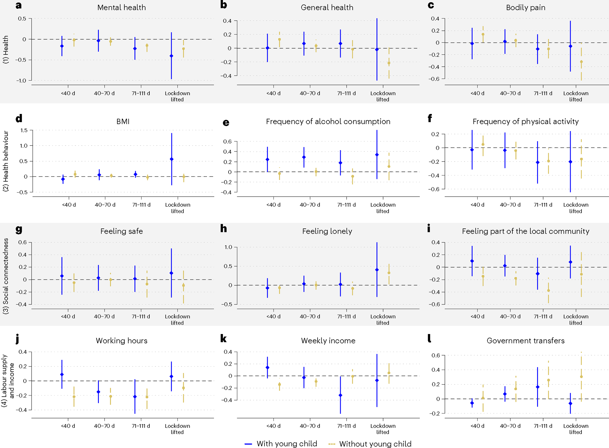
This dose–response analysis revealed that longer exposure to lockdown had no consistent effect across domains (Figs. 4 and 5). Instead, we found heterogeneous trends over exposure time. For mothers, the mental health penalties of lockdown faded over time: after plummeting significantly by −0.34 s.d. (P = 0.005, 95% CI = −0.35 to 1.11) in the early days of lockdown, mental health was unaffected in individuals interviewed at the end of the lockdown. The treatment effects were not statistically different between the groups (Fig. 4a; Δ = 0.24 s.d., P = 0.111, F = 2.54). In contrast, mothers’ general health worsened over the lockdown period. At the beginning of lockdown, there were no statistically significant effects on general health, but by the end of lockdown general health had significantly dropped by over 0.3 s.d. (P = 0.006, 95% CI = −0.53 to −0.09), with a significant difference between the two groups (Fig. 4b; Δ = 0.28 s.d., P = 0.033, F = 4.52). Working hours also significantly declined over time (Fig. 4h), with zero treatment effects at the beginning and a significant drop of 0.27 s.d. by the end of lockdown (P = 0.006, 95% CI = −0.46 to −0.08), where treatment effects significantly differed between the two groups (Δ = 0.26 s.d., P = 0.030, F = = 4.71). Mothers’ weekly incomes were not affected early in the lockdown but significantly declined by the end of lockdown (Fig. 4i), although again the two groups did not differ in a statistical sense (Δ = 0.22 s.d., P = 0.115, F = 0.115). This decline was not compensated for by an increase in government transfers as lockdown progressed (Fig. 4j; β = 0.15 s.d., P = 0.417, F = 0.66). Other relevant outcomes were affected uniformly throughout lockdown (for example, feeling safe).

Fig. 4 |. Lockdown treatment effect (expressed in s.d.) for women for selected outcomes according to length of exposure and family status.

Estimated treatment effects of lockdown for different exposure lengths to lockdown for women. a, Mental health. b, General health. c, Bodily pain. d, BMI. e, Frequency of alcohol consumption. f, Frequency of physical activity. g, Feeling safe. h, Feeling lonely. i, Feeling part of the local community. j, Working hours. k, Weekly income. l, Government transfers. Spikes represent the 95% CIs. Estimates are expressed in s.d. (from 0 mean) obtained from separate difference-in-differences regressions of a specific outcome on a treatment group indicator. We used the same specification as the benchmark model (Fig. 2), but the treatment indicator (wave 20 × Melbourne) was interacted with four dummy variables, each of which presents a different exposure length to lockdown: fewer than 40 d; 40–70 d; 71–111 d; and the days after lockdown was lifted. Note that vertical axes vary across the panels. Each panel presents results for different outcomes. The sample sizes for each estimation are reported in Supplementary Table 16. Supplementary Table 22 presents the full model results.

Fig. 5 |. Estimated treatment effect of lockdown (expressed in s.d.) for men and for selected outcomes according to the length of exposure and family status.

Estimated treatment effects of lockdown for different exposure lengths to lockdown for men. a, Mental health. b, General health. c, Bodily pain. d, BMI. e, Frequency of alcohol consumption. f, Frequency of physical activity. g, Feeling safe. h, Feeling lonely. i, Feeling part of the local community. j, Working hours. k, Weekly income. l, Government transfers. Spikes represent the 95% CIs. Estimates are expressed in s.d. (from 0 mean), obtained from separate difference-in-differences regressions of a specific outcome on a treatment group indicator. We used the same specification as the benchmark model (Fig. 2), but the treatment indicator (wave 20 × Melbourne) was interacted with four dummy variables, each of which presents a different exposure length to lockdown: fewer than 40 d; 40–70 d; 71–111 d; and the days after lockdown was lifted. Note that the vertical axes vary across panels. Each panel presents results for different outcomes. The sample sizes for each estimation are reported in Supplementary Table 16. Supplementary Table 23 presents the full model results.

For fathers, longer lockdown exposure also had additional effects. Their BMI significantly increased by the end of lockdown relative to the beginning of lockdown (Fig. 5d; Δ = −0.15 s.d., P = 0.046, F = 3.98). As seen in mothers, fathers also reduced their working hours only at later stages of the lockdown, where treatment effects between early and late lockdown groups differed significantly (Fig. 5k; Δ = 0.31 s.d., P = 0.034, F = 4.51). Fathers’ incomes dropped significantly only by the end of lockdown (Fig. 5k; β = −0.32 s.d., P = 0.043, 95% CI = −0.63 to −0.01).

As the lockdown went on, men without dependent children also showed signs of harm, with significant differences between early and late lockdown groups. While their general health (Δ = 0.15 s.d., P = 0.045, F = = 4.02) and physical activity (Δ = 0.24 s.d., P = 0.022, F = 5.25) progressively declined, government transfers progressively increased (Δ = 0.29 s.d., P = 0.049, F = 3.89).

Could other factors have explained our findings?

One could argue that the common trend assumption may have been violated if we believed that the onset of new infections in Melbourne—roughly more than 100 infections per day—could have caused anxiety about the prospects of getting seriously ill and direct health problems from COVID-19 infection. In supplementary analyses (Supplementary Table 12, panels A–C), we showed that such concerns were largely unfounded. While Melbournian women and men were more likely than Sydneysiders to think that they would get infected with COVID-19 (for women: 15.2% implied change, linear probability model estimate γ = 3.76, P < 0.001, 95% CI = 1.96 to 5.56; for men: 9.0% implied change, γ = 2.10, P = 0.024, 95% CI = 0.27 to 3.92), consistent with expectations of an outbreak with community transmission, they did not have a higher probability of an actual COVID-19 infection at the time of the interview (for women: γ = 0, P = 0.721, 95% CI = −0 to 0; for men: γ = −0, P = 0.362, 95% CI = −0.01 to 0). Nor did they expect to be more likely to get seriously ill if infected (for women: γ = 0.93, P = 0.407, 95% CI = −1.23 to 3.11; for men: γ = −1.78, P = 0.102, 95% CI = −3.92 to 0.35).

Additional analysis also ruled out that Melbournians entered the second lockdown period significantly more harmed financially by the first lockdown that also affected Sydneysiders. A difference-in-differences model, which used the same specification as our benchmark model, but used previous financial year disposal total incomes (which included incomes up until June 2020) as the outcome variable, showed that neither female (β = −0.03 s.d., P = 0.411, 95% CI = −0.1 to 0.04) nor male (β = 0.03 s.d., P = 0.496, 95% CI = −0.05 to 0.10) Melbournians experienced greater declines in income relative to the previous financial year than Sydneysiders (Supplementary Table 12, panel D).

Discussion

We conclude from our analysis that hard lockdown, the cornerstone intervention of zero-COVID policies, had some statistically significant effects on Melbournians on average, but treatment effects were mostly small in magnitude (<0.2 s.d.). But the exploratory heterogeneity analysis suggests that the policy may have come with larger penalties for parents, particularly for mothers. Mothers experienced moderately sized mental health penalties (−0.27 s.d.), which occurred despite sizeable improvements in perceptions of safety (0.27 s.d.). Some outcomes for mothers worsened by the length of the lockdown, where significant penalties emerged only later during the lockdown. By the end of lockdown, mothers had significant penalties to their general health (−0.31 s.d.) and BMI (0.14 s.d.) and labour supply (−0.27 s.d.). Although statistically significant, mental health penalties were observable only in the first two-thirds of the lockdown, with magnitudes surpassing 0.30 s.d.; mothers felt significant increases in loneliness both at the beginning (0.27 s.d.) and the end of the lockdown (0.29 s.d.).

The effect sizes imply that mothers reduced their mental health by over 7.5%. By the end of lockdown, mothers reduced their labour supply by 5.5 h worked per week, general health levels dropped by 9% and loneliness levels increased by almost 19.4%, each calculated relative to Melbourne’s long-term average pre-lockdown (Table 1). Their feelings of safety increased only by around 5%. Fathers increased their alcohol consumption frequency in a way that moved them to drinking 1–2 d a week rather than once per week. While the frequency increase of alcohol consumption was the same throughout lockdown, by the end of lockdown, fathers also experienced a significant reduction in working hours by 0.22 s.d., which translates into 4.4 h worked less per week. They also experienced by the end of lockdown a loss in current gross salaries and wages of −0.32 s.d., which translates to AU$280 less per week.

Increases in mental health problems, loneliness and alcohol consumption are potentially harmful responses to social isolation. Why were mainly mothers and fathers affected by the lockdown? Mothers in particular experienced declines in their emotional well-being throughout the lockdown. One explanation for this negative response is that mothers carried a greater mental load than usual during lockdown. In general, mothers carry a high cognitive load to schedule, plan and organize family activities, and are known to work more hours in the household than fathers⁴⁴. This cognitive load probably becomes a mental load when this daily process is combined with stress and worry. Mothers during lockdown were more likely to take responsibility for homeschooling, which would have added additional workload^36–38. Mothers may also have been affected by the regular presence of their partners. Fathers unambiguously increased the frequency with which they drank alcohol during lockdown, a risky health behaviour. This combined presence of drinking partners in combination with social isolation may have increased family discord or exposed women to more violence in the home. Concerns over increased interpersonal violence were reported early in context of the costs of lockdown⁴⁵ and heightened case numbers were expected for Australia by July 2020 (ref. 46). However, our analysis confirmed that mothers, on average, felt safer during lockdown. In supplementary analyses, we showed that neither mothers nor fathers were significantly less satisfied with their partners (Supplementary Table 13). Thus, we ruled out that the harm experienced by mothers was driven by greater risks and partner dissatisfaction in the home. More probably, mothers were simply burdened by additional working hours in the home, which is consistent with a non-compensated, potentially voluntary reduction in formal working hours that we observed in our data.

One concern is that statistically non-significant results in other vulnerable groups were produced by our sample size. The sample size varied for each outcome in the main and subgroup analyses. Using a conservative approach, based on the number of individuals rather than observations, the minimum sample size for one sex was for the outcome alcohol consumption, where 927 Sydney men and 1,178 Melbourne men responded in 2020. Without accounting for weighting and with a power of 0.9, these sample sizes would allow a small effect size difference of 0.14 s.d. to be detected with statistical significance in this outcome. For the other outcomes with larger samples, even smaller differences would be statistically significant. However, this could explain why some of the estimated treatment effects for fathers were not statistically significant and no different from the ones estimated for mothers.

Another limitation of our analysis is that adjusting for the many hypotheses tested in the subgroup analyses rendered some treatment effects, strictly speaking (α < 0.05), statistically non-significant for mothers. Thus, our flexible estimation model, which controls for many confounders, city-specific time trends and individual-specific fixed effects, in combination with a large number of hypotheses tested, comes at the cost of producing some uncertainty about our findings.

Another limitation is that our findings may not be generalizable because we focused on one city in the world, which returned to zero new COVID-19 infections through a hard and, at the time, uniquely long lockdown that also closed schools. For some domains, outcomes worsened only with the length of lockdown. So, it may be hard to generalize our findings to other jurisdictions and lockdown settings, where lockdown was shorter^20,29,32 or confounded by financial distress and high burden of disease²⁹, or where schools remained open. Our conclusions about the net human cost of lockdown may be compromised by incomplete information about the plight of children and other relevant outcomes. Penalties may have been larger if considering the likely learning and well-being losses for children during lockdown. Lockdown penalties may have been offset by other positive outcomes that we were not able to observe, such as community resilience to or empathy developed due to the experience of adverse events. However, our findings suggest that in similar settings, where there is a strong social preference for saving lives through lockdowns, policy responses may need to focus on mitigating the effects of hard lockdowns on the parents of school-aged children, as emphasized elsewhere³⁰.

Methods

Lockdown rollout

Information on Australia’s pandemic strategy and rollout dates of lockdowns is available in reports of the Australian Institute of Health and Welfare⁴⁷ (Table 1.2) and Fair Work Commission⁴⁸. The JobKeeper programme was a generous fiscal stimulus package that was rolled out early during the first lockdown in Australia⁴⁹. Melbourne’s lockdown was facilitated by both voluntary and mandatory mobility restrictions, according to Facebook Data for Good on mobility trends in Victoria⁵⁰. On 1 July, lockdowns were announced for specific postcodes, decreasing mobility in Melbourne by 29%. Stage 4 restrictions were introduced in Greater Melbourne on 1 August, further reducing mobility by 52%. Mobility was less restricted outside the Greater Melbourne area, with evidence that mobility was reduced only by 15% on 1 July 2021 and by a further 34% on 1 August 2020 (ref. 50). Our own previous work found that people were more affected by lockdown in the Melbourne metropolitan areas⁵¹. It is for this reason that we focused the analysis on greater metropolitan areas.

Data

We sourced data from the HILDA Survey. This household panel commenced in 2001 (wave 1) with a nationally representative sample of Australian households⁵². The first-wave sample consisted of 13,969 participants from 7,682 households, which was then followed on an annual basis with all members of those initial households aged 15 years or older, or persons who joined the household later. Individuals gave oral informed consent for participation in the study. Additionally, consent was sought from parents or guardians before seeking the involvement of household members aged younger than 18 years. Ethics approval was granted by the Human Research Ethics Committee of the University of Melbourne in 2001 and has been updated or renewed on annual basis since (ID no. 1955879).

In 2011, the sample was refreshed with an additional 2,153 households. Sample loss and attrition were low, with re-interview rates rising from 87% in wave 2 to over 95% by wave 8 and remaining above that level in subsequent waves⁵³.

The data collection process begins every year in August and ends the following February. Before wave 20, more than 90% of interviews were conducted face to face. During the pandemic year, 96% of all person interviews in wave 20 were conducted over the phone.

In addition to an individual interview, respondents were asked to complete a separate self-completion questionnaire. Before wave 20, this was a paper form that was either collected by the interviewer or returned in the post. In wave 20, an online option was provided, without affecting return rates (91.9% in 2020 versus 92.1% in 2019).

Sample

We used ten waves of data spanning the period from 2011 to 2020. After restricting this sample to individuals living in either metropolitan Melbourne or Sydney, the maximum sample size consisted of 9,441 individuals or 60,108 PYO (Table 1; stage 1). Analytical sample sizes were slightly smaller due to missing data (60,031 PYO, stage 2) and varied with the outcome of interest (stage 3). The final estimation sample included all individuals with at least two repeat observations, ranging between 45,053 PYO (frequency of alcohol consumption) and 59,236 PYO (labour market outcomes) (stage 4).

Additional information on health outcome measures

From the Medical Outcomes Study Questionnaire Short Form 36 (inventory), one of the most widely used self-completion measures of health, we derived three measures of health. These are mental health, general health and bodily pain. Previous research showed that these items in the HILDA Survey have good psychometric properties⁵⁴. These measures were collected in the HILDA Survey using the self-completion questionnaire.

Estimation model

We used methods from the policy evaluation literature^55–58 to estimate the causal impact of lockdown on human life. We exploited the fact that lockdown was implemented only in Melbourne (Victoria) and nowhere else in the country, and that individuals could not leave Melbourne or Victoria easily to avoid lockdown rules. The treatment group consisted of individuals who were located in the greater metropolitan area of Melbourne during lockdown. The control group consisted of individuals who were located in the greater metropolitan area of Sydney during the time when Melbourne was locked down. We chose city areas as the focus of the analysis because lockdowns were more likely to be enforced strictly in those areas.

Like the few other studies that estimated the causal impact of lockdown^29,32, our models were based on a difference-in-differences specification, which compared changes over time in the treatment group with changes over time in the control group, while holding time trends in outcomes constant in both treatment and control groups. Each model was estimated separately for men and women.

We regressed outcome ${Y_{it}}^k(k=1,\dots ,12$ outcomes, three in each of four domains) on a non-linear year (which refers to the survey wave) trend (vector ${\mathrm{Y}\mathrm{e}\mathrm{a}\mathrm{r}}_t$, dummy variables for each year, base 2019), a dummy variable for living in ${\mathrm{M}\mathrm{e}\mathrm{l}\mathrm{b}\mathrm{o}\mathrm{u}\mathrm{r}\mathrm{n}\mathrm{e}}_{it}$ in year $t$, an interaction effect between non-linear year trends and ${\mathrm{M}\mathrm{e}\mathrm{l}\mathrm{b}\mathrm{o}\mathrm{u}\mathrm{r}\mathrm{n}\mathrm{e}}_{it}$ (=1 if lived in Melbourne in year $t$, =0 if lived in Sydney in year $t$) and a range of control variables $X_{it}$ that can vary across time. For simplicity, we dropped the $k$ outcome superscript:

$$\begin{gathered} Y_{it}={\beta }_0+{\text{Year}}_t^{\prime }{\mathit{\beta }}_{\mathbf{1}}+{\beta }_2{\text{Melbourne}}_{it} \\ +{\left({\text{Melbourne}}_{it}x{\text{Year}}_t\right)}^{\prime }{\mathit{\beta }}_{\mathbf{3}}+X_{it}^{\prime }\mathit{\mu }+{\alpha }_i+{\epsilon }_{it} \end{gathered}$$ (1)

$X_{it}$ includes the following dummy variables: age group; number of individuals in the household; number of children in the household younger than 25 years; highest level of education; and marital status categories. We also controlled for the month when and how (telephone, face to face) the interview was conducted. Controlling for the interview timing is potentially important because lockdown may have shifted the interview timing of those residing in Melbourne in 2020. Although we found that the interview schedule distribution hardly changed from previous years, there was a small difference noteworthy for the 2020 interviews: the interviews in Melbourne were completed slightly earlier than in Sydney (Supplementary Fig. 2), whereas in 2019 the rollout dates were identical. This probably reflects Melbournians, locked inside their homes, being easier to reach. $\mathbf{\mu }$ is a vector of parameters to be estimated. Individual fixed effects are captured in ${\alpha }_i$.

This model allows for city-specific time trends in outcome $Y_{it}$. The coefficients in ${\mathit{\beta }}_{\mathbf{1}}$ capture the time trend for individuals in Sydney. The coefficient ${\beta }_2$ captures the effect of living in Melbourne in any given year $t$. The coefficient in ${\mathit{\beta }}_{\mathbf{3}}$ captures the time trend in outcome $Y_{it}$ for individuals in Melbourne (${\mathrm{M}\mathrm{e}\mathrm{l}\mathrm{b}\mathrm{o}\mathrm{u}\mathrm{r}\mathrm{n}\mathrm{e}}_{it}=1$). The coefficient of interest is ${\beta }_{\mathrm{3,2020}}$, which measures the change in outcome $Y_{it}$ in 2020 for individuals in Melbourne, and thus in lockdown, relative to their 2019 outcomes, all other things being equal. Under the null hypothesis, we tested ${\beta }_{\mathrm{3,2020}}=0$ against a two-sided alternative hypothesis $\left({\beta }_{\mathrm{3,2020}}\ne 0\right)$. We rejected the null hypothesis for a statistical significance level of $\alpha =0.05$. In all estimations, data distribution was assumed to be normal but this was not formally tested.

All models used survey component-specific sample probability weights to make the samples representative for the population in each wave. Standard errors were clustered at the household level to adjust for non-independent observations per household. All estimates were reported as standardized coefficients interpreted as a percentage s.d. difference in outcomes before and during lockdown for the treatment group relative to the control group.

A typical difference-in-differences model identified the causal impact of lockdown under the parallel trends assumption. This means that trends in outcomes should be the same between treatment and control groups in the absence of lockdown. To test for the parallel trends assumption, it is common to test for the statistical significance of all pretreatment trends for the treatment group. Under the null hypothesis of no differential pretreatment trends, we tested for: ${\beta }_{\mathrm{3,2018}}={\beta }_{\mathrm{3,2017}}={\beta }_{\mathrm{3,2016}}={\beta }_{\mathrm{3,2015}}={\beta }_{\mathrm{3,2014}}={\beta }_{\mathrm{3,2013}}={\beta }_{\mathrm{3,2012}}={\beta }_{\mathrm{3,2011}}=0$, against the alternative hypothesis that at least one of these coefficients was significantly different from 0. We also showed these coefficients in what the literature calls an event-study framework and present placebo tests that help to rule out that significant treatment effects are produced by underlying time trends^57,58.

In the statistical inference, we tested for many null hypotheses for both women and men in each domain in the full sample (three null hypotheses) and within each domain across five vulnerable groups (three outcomes × five groups per domain which equals 15 null hypotheses tested simultaneously). Allowing for an accepted significance level of $\alpha =0.05$, it is possible to find one statistically significant treatment effect in the heterogeneity analysis per domain simply by chance (15 × 0.05 = 0.75 times). We thus present in a robustness check P values adjusted for MHT using the flexible step down method suggested by Romano and Wolf^59,60, with a similar adjustment logic (per domain, per sex) as proposed by Campbell et al.⁶¹. These adjusted values account for the family-wise error rate (that is, the probability of making at least one type I error when performing our three hypothesis tests per domain per sex, or 15 hypothesis tests per domain per sex across five vulnerable groups) that conventional P values do not.

Finally, in the above model, the same individual could be both in the treatment group in 2020 and in the control group in 2019 (or vice versa) because the model allows location status to change over time. However, this modelling approach does not alter our conclusions. We estimated a similar difference-in-differences model with individual fixed effects but held location and thus treatment group status fixed over time. Our conclusions were unaffected when using this model.

Reporting summary

Further information on research design is available in the Nature Portfolio Reporting Summary linked to this article.

Data availability

This paper uses unit record data from the HILDA Survey, conducted by the Melbourne Institute of Applied Economic and Social Research on behalf of the Australian Government DSS (release 20, https://dataverse.ada.edu.au/dataset.xhtml?persistentId=doi:10.26193/PI5LPJ, ADA Dataverse). The data used are available free of charge to researchers through the National Centre for Longitudinal Data Dataverse at the ADA (https://dataverse.ada.edu.au/dataverse/ncld). Access is subject to approval by the Australian Government DSS and is conditional on signing a licence specifying the terms of use. Source data are provided with this paper.

References

- 1.Haug N et al. Ranking the effectiveness of worldwide COVID-19 government interventions. Nat. Hum. Behav. 4, 1303–1312 (2020). [DOI] [PubMed] [Google Scholar]
- 2.Desvars-Larrive A et al. A structured open dataset of government interventions in response to COVID-19. Sci. Data 7, 285 (2020). [DOI] [PMC free article] [PubMed] [Google Scholar]
- 3.Sandford A Coronavirus: half of humanity now on lockdown as 90 countries call for confinement. Euronews https://www.euronews.com/2020/04/02/coronavirus-in-europe-spain-s-death-toll-hits-10-000-after-record-950-new-deaths-in-24-hou (02 April 2020).
- 4.Dehning J et al. Inferring change points in the spread of COVID-19 reveals the effectiveness of interventions. Science 369, eabb9789 (2020). [DOI] [PMC free article] [PubMed] [Google Scholar]
- 5.Flaxman S et al. Estimating the effects of non-pharmaceutical interventions on COVID-19 in Europe. Nature 584, 257–261 (2020). [DOI] [PubMed] [Google Scholar]
- 6.Burki TK Herd immunity for COVID-19. Lancet Respir. Med. 9, 135–136 (2021). [DOI] [PMC free article] [PubMed] [Google Scholar]
- 7.Alwan NA et al. Scientific consensus on the COVID-19 pandemic: we need to act now. Lancet 396, e71–e72 (2020). [DOI] [PMC free article] [PubMed] [Google Scholar]
- 8.Baker M, Wilson N & Blakely T Elimination could be the optimal response strategy for covid-19 and other emerging pandemic diseases. BMJ 371, m4907 (2020). [DOI] [PubMed] [Google Scholar]
- 9.Lenzer J Covid-19: group of UK and US experts argues for “focused protection” instead of lockdowns. BMJ 371, m3908 (2020). [DOI] [PubMed] [Google Scholar]
- 10.Pachetti M Impact of lockdown on Covid-19 case fatality rate and viral mutations spread in 7 countries in Europe and North America. J. Transl. Med. 18, 338 (2020). [DOI] [PMC free article] [PubMed] [Google Scholar]
- 11.Oliu-Barton M et al. SARS-CoV-2 elimination, not mitigation, creates best outcomes for health, the economy, and civil liberties. Lancet 397, 2234–2236 (2021). [DOI] [PMC free article] [PubMed] [Google Scholar]
- 12.Dave D, Friedson AI, Matsuzawa K & Sabia JJ When do shelter-in-place orders fight COVID-19 best? Policy heterogeneity across states and adoption time. Econ. Inq. 59, 29–52 (2021). [DOI] [PMC free article] [PubMed] [Google Scholar]
- 13.Blakely T et al. The probability of the 6-week lockdown in Victoria (commencing 9 July 2020) achieving elimination of community transmission of SARS-CoV-2. Med. J. Aust. 213, 349–351 (2020). [DOI] [PubMed] [Google Scholar]
- 14.Berry CR, Fowler A, Glazer T, Handel-Meyer S & MacMillen A Evaluating the effects of shelter-in-place policies during the COVID-19 pandemic. Proc. Natl Acad. Sci. USA 118, e2019706118 (2021). [DOI] [PMC free article] [PubMed] [Google Scholar]
- 15.Meo SA et al. Impact of lockdown on COVID-19 prevalence and mortality during 2020 pandemic: observational analysis of 27 countries. Eur. J. Med. Res. 25, 56 (2020). [DOI] [PMC free article] [PubMed] [Google Scholar]
- 16.Gibson J Government mandated lockdowns do not reduce COVID-19 deaths: implications for evaluating the stringent New Zealand response. N. Z. Econ. 56, 17–28 (2022). [Google Scholar]
- 17.Normile D Can ‘zero COVID’ countries continue to keep the virus at bay once they reopen? Successful strategies used in Asia and the Pacific may not be sustainable in the long run. Science 373, 1294–1295 (2021). [DOI] [PubMed] [Google Scholar]
- 18.Robinson E, Sutin AR, Daly M & Jones A A systematic review and meta-analysis of longitudinal cohort studies comparing mental health before versus during the COVID-19 pandemic in 2020. J. Affect. Disord. 296, 567–576 (2022). [DOI] [PMC free article] [PubMed] [Google Scholar]
- 19.Witteveen D & Velthorst E Economic hardship and mental health complaints during COVID-19. Proc. Natl Acad. Sci. USA 117, 27277–27284 (2020). [DOI] [PMC free article] [PubMed] [Google Scholar]
- 20.Pierce M et al. Mental health before and during the COVID-19 pandemic: a longitudinal probability sample survey of the UK population. Lancet Psychiatry 7, 883–892 (2020). [DOI] [PMC free article] [PubMed] [Google Scholar]
- 21.Brooks SK et al. The psychological impact of quarantine and how to reduce it: rapid review of the evidence. Lancet 395, 912–920 (2020). [DOI] [PMC free article] [PubMed] [Google Scholar]
- 22.Varga TV et al. Loneliness, worries, anxiety, and precautionary behaviours in response to the COVID-19 pandemic: a longitudinal analysis of 200,000 Western and Northern Europeans. Lancet Reg. Health Eur. 2, 100020 (2021). [DOI] [PMC free article] [PubMed] [Google Scholar]
- 23.Brodeur A, Clark AE, Fleche S & Powdthavee N COVID-19, lockdowns and well-being: evidence from Google Trends. J. Public Econ. 193, 104346 (2021). [DOI] [PMC free article] [PubMed] [Google Scholar]
- 24.Armbruster S & Klotzbücher V Lost in lockdown? COVID-19, social distancing, and mental health in Germany. CEPR https://cepr.org/node/390474 (2020). [Google Scholar]
- 25.Bajos N et al. When lockdown policies amplify social inequalities in COVID-19 infections: evidence from a cross-sectional population-based survey in France. BMC Public Health 21, 705 (2021). [DOI] [PMC free article] [PubMed] [Google Scholar]
- 26.Wright L, Steptoe A & Fancourt D Are we all in this together? Longitudinal assessment of cumulative adversities by socioeconomic position in the first 3 weeks of lockdown in the UK. J. Epidemiol. Community Health 74, 683–688 (2020). [DOI] [PMC free article] [PubMed] [Google Scholar]
- 27.Perry BL, Aronson B & Pescosolido BA Pandemic precarity: COVID-19 is exposing and exacerbating inequalities in the American heartland. Proc. Natl Acad. Sci. USA 118, e2020685118 (2021). [DOI] [PMC free article] [PubMed] [Google Scholar]
- 28.Adams-Prassl A, Boneva T, Golin M & Rauh C Inequality in the impact of the coronavirus shock: evidence from real time surveys. J. Public Econ. 189, 104245 (2020). [Google Scholar]
- 29.Adams-Prassl A, Boneva T, Golin M & Rauh C The impact of the coronavirus lockdown on mental health: evidence from the United States. Econ. Policy 37, 139–155 (2022). [Google Scholar]
- 30.Croda E & Grossbard S Women pay the price of COVID-19 more than men. Rev. Econ. Househ. 19, 1–9 (2021). [DOI] [PMC free article] [PubMed] [Google Scholar]
- 31.Yavorsky JE, Qian Y & Sargent AC The gendered pandemic: the implications of COVID-19 for work and family. Sociol. Compass 15, e12881 (2021). [DOI] [PMC free article] [PubMed] [Google Scholar]
- 32.Serrano-Alarcón M, Kentikelenis A, Mckee M & Stuckler D Impact of COVID-19 lockdowns on mental health: evidence from a quasi-natural experiment in England and Scotland. Health Econ. 31, 284–296 (2022). [DOI] [PMC free article] [PubMed] [Google Scholar]
- 33.Johnston R, Mohammed A & van der Linden C Evidence of exacerbated gender inequality in child care obligations in Canada and Australia during the COVID-19 pandemic. Politics Gend. 16, 1131–1141 (2020). [Google Scholar]
- 34.Bryson H et al. Clinical, financial and social impacts of COVID-19 and their associations with mental health for mothers and children experiencing adversity in Australia. PLoS ONE 16, e0257357 (2021). [DOI] [PMC free article] [PubMed] [Google Scholar]
- 35.Sevilla A & Smith S Baby steps: the gender division of childcare during the COVID-19 pandemic. Oxf. Rev. Econ. Policy 36, S169–S186 (2020). [Google Scholar]
- 36.Alon T, Doepke M, Olmstead-Rumsey J & Tertilt M This Time It’s Different: the Role of Women’s Employment in a Pandemic Recession. NBER Working Paper Series 27660 (NBER, 2020). [Google Scholar]
- 37.Belot M et al. Unequal consequences of Covid 19: representative evidence from six countries. Rev. Econ. Househ. 19, 769–783 (2021). [DOI] [PMC free article] [PubMed] [Google Scholar]
- 38.Collins C, Landivar LC, Ruppanner L & Scarborough WJ COVID-19 and the gender gap in work hours. Gend. Work Organ. 28, 101–112 (2021). [DOI] [PMC free article] [PubMed] [Google Scholar]
- 39.Craig L & Churchill B Working and caring at home: gender differences in the effects of Covid-19 on paid and unpaid labor in Australia. Fem. Econ. 27, 310–326 (2021). [Google Scholar]
- 40.Hupkau C & Petrongolo B Work, care and gender during the COVID-19 crisis. Fisc. Stud. 41, 623–651 (2020). [DOI] [PMC free article] [PubMed] [Google Scholar]
- 41.Smith P Hard lockdown and a “health dictatorship”: Australia’s lucky escape from covid-19. BMJ 371, m4910 (2020). [DOI] [PubMed] [Google Scholar]
- 42.Lane CR et al. Genomics-informed responses in the elimination of COVID-19 in Victoria, Australia: an observational, genomic epidemiological study. Lancet Public Health 6, e547–e556 (2021). [DOI] [PMC free article] [PubMed] [Google Scholar]
- 43.Horton R Offline: the case for no-COVID. Lancet 397, 359 (2021). [DOI] [PMC free article] [PubMed] [Google Scholar]
- 44.Dean L, Churchill B & Ruppanner L The mental load: building a deeper theoretical understanding of how cognitive and emotional labor overload women and mothers. Community Work Fam. 25, 13–29 (2022). [Google Scholar]
- 45.Usher K, Bhullar N, Durkin J, Gyamfi N & Jackson D Family violence and COVID-19: increased vulnerability and reduced options for support. Int. J. Ment. Health Nurs. 29, 549–552 (2020). [DOI] [PMC free article] [PubMed] [Google Scholar]
- 46.Boxall H, Morgan A & Brown R The prevalence of domestic violence among women during the COVID-19 pandemic. Australas. Polic. 12, 38–46 (2020). [Google Scholar]
- 47.The First Year of COVID-19 in Australia: Direct and Indirect Health Effects (Australian Institute of Health and Welfare, 2021). [Google Scholar]
- 48.Information Note—Government Responses to COVID-19 Pandemic (Updated 23 September 2021) (Fair Work Commission, 2021). [Google Scholar]
- 49.Walkowiak E JobKeeper: the Australian short-time work program. Aust. J. Public Adm. 80, 1046–1053 (2021). [Google Scholar]
- 50.Zachreson C, Rebulli N, Mitchell L, Tomko M & Geard N What mobility data can tell us about COVID-19 lockdowns. InSight+ https://insightplus.mja.com.au/2020/41/what-mobility-data-can-tell-us-about-covid-19-lockdowns/ (19 October 2020). [Google Scholar]
- 51.Butterworth P, Schurer S, Trinh T-A, Vera-Toscano E & Wooden M Effect of lockdown on mental health in Australia: evidence from a natural experiment analysing a longitudinal probability sample survey. Lancet Public Health 7, e427–e436 (2022). [DOI] [PMC free article] [PubMed] [Google Scholar]
- 52.Watson N & Wooden M The Household, Income and Labour Dynamics in Australia (HILDA) Survey. Jahrb. Natl Okon. Stat. 241, 131–141 (2020). [Google Scholar]
- 53.Summerfield M et al. HILDA User Manual—Release 20 (Melbourne Institute of Applied Economic and Social Research, 2021); https://melbourneinstitute.unimelb.edu.au/hilda/for-data-users/user-manuals [Google Scholar]
- 54.Butterworth P & Crosier T The validity of the SF-36 in an Australian National Household Survey: demonstrating the applicability of the Household Income and Labour Dynamics in Australia (HILDA) Survey to examination of health inequalities. BMC Public Health 4, 44 (2004). [DOI] [PMC free article] [PubMed] [Google Scholar]
- 55.Wing C, Simon K & Bello-Gomez RA Designing difference in difference studies: best practices for public health policy research. Ann. Rev. Public Health 39, 453–469 (2018). [DOI] [PubMed] [Google Scholar]
- 56.de Vocht F et al. Conceptualising natural and quasi experiments in public health. BMC Med. Res. Methodol. 21, 32 (2021). [DOI] [PMC free article] [PubMed] [Google Scholar]
- 57.Cunningham S Causal Inference: The Mixtape (Yale Univ. Press, 2021). [Google Scholar]
- 58.de Chaisemartin C & D’Haultfoeuille X Two-way fixed effects estimators with heterogeneous treatment effects. Am. Econ. Rev. 110, 2964–2996 (2020). [Google Scholar]
- 59.Romano JP & Wolf M Exact and approximate stepdown methods for multiple hypothesis testing. J. Am. Stat. Assoc. 100, 94–108 (2005). [Google Scholar]
- 60.Romano JP & Wolf M Stepwise multiple testing as formalized data snooping. Econometrica 73, 1237–1282 (2005). [Google Scholar]
- 61.Campbell F et al. Early childhood investments substantially boost adult health. Science 343, 1478–1485 (2014). [DOI] [PMC free article] [PubMed] [Google Scholar]
Associated Data
This section collects any data citations, data availability statements, or supplementary materials included in this article.
Supplementary Materials
Data Availability Statement