Abstract
Dicrotic Notch (DN), one of the most significant and indicative features of the arterial blood pressure (ABP) waveform, becomes less pronounced and thus harder to identify as a matter of aging and pathological vascular stiffness. Generalizable and automatic DN identification for such edge cases is even more challenging in the presence of unexpected ABP waveform deformations that happen due to internal and external noise sources or pathological conditions that cause hemodynamic instability. We propose a physics-aware approach, named Physiowise (PW), that first employs a cardiovascular model to augment the original ABP waveform and reduce unexpected deformations, then apply a set of predefined rules on the augmented signal to find DN locations. We have tested the proposed method on in-vivo data gathered from 14 pigs under hemorrhage and sepsis study. Our result indicates 52% overall mean error improvement with 16% higher detection accuracy within the lowest permitted error range of 30ms. An additional hybrid methodology is also proposed to allow combining augmentation with any application-specific user-defined rule set.
Keywords: Model-based approaches, Rule-based approaches, Dicrotic Notch identification, Hemorrhage, Sepsis
1. INTRODUCTION
Arterial Blood Pressure (ABP) waveform carries critical information on both the cardiovascular system and its underlying control system [1]. Extraction of such information has been the target of research in a wide range of healthcare applications such as early hemodynamic impairment detection [2], hypotension prediction [3], and fluid responsiveness analysis in critical care [4]. Dicrotic Notch (DN) is a clinically significant feature of the ABP waveform that patterns a secondary up-rise in the pressure signal after the main maxima. The automatic DN detection becomes challenging as its morphology ranges from a clear-cut pressure up-rise to a diminished slope change. The problem is intensified under signal deformations due to the presence of many dynamic actors, such as internal and external noise sources or pathological conditions, affecting the ABP waveform.
Previously established DN detection methods, categorized as rule-based or model-based approaches, commonly target DN detection on normal ABP waveforms and ignore the edge cases. As these edge scenarios become more prevalent with aging and underlying conditions that increase the vascular beds’ stiffness or hemodynamic instability, automatic DN detection methods may fail to capture patterns that do not comply with their preset assumptions.
We propose a physics-aware approach, Physiowise (PW), that enhances generalizability under ABP waveform deformations. Figure 1 depicts the overall view of the proposed method. PW is a combination of modelbased and rule-based methods. The model-based data augmentation aims at synthesizing the deformed ABP waveforms closely while omitting unexpected patterns that do not comply with the model’s assumptions. This results in a much more controlled fluctuation on the augmented ABP waveform in comparison to the original ABP waveform. The proposed rule-based algorithm can generate the DN placements using this augmented waveform (Figure 1(a)). A user-defined rule-based method can also be integrated with our approach (Figure 1(b)). Such a rule-based method is applied to both original and augmented data to generate two sets of DN placement markers. A voting algorithm receives these identified DN placements and decides the final DN identification output.
Fig. 1.
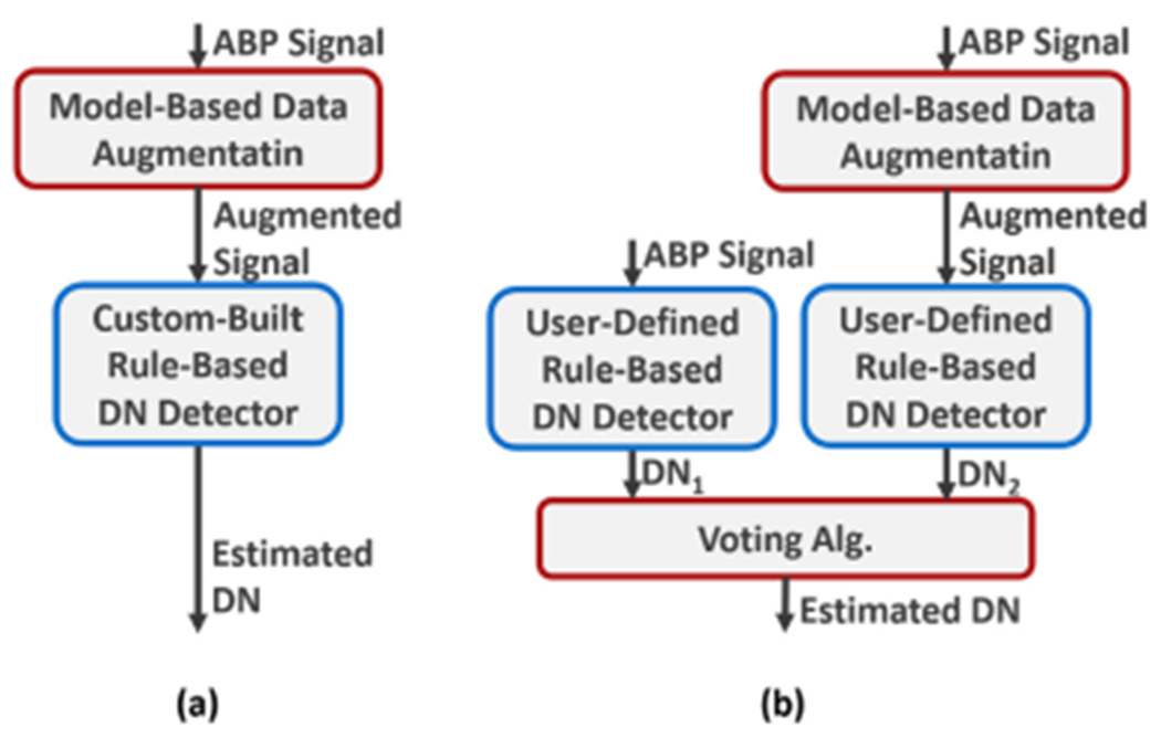
High-level explanation of the proposed approach. (a) PW methodology. (b) Hybrid voting method with a user-defined rule-based algorithm.
We propose a novel parameter optimization technique that can highlight DN location under waveform deformations, a scenario that has not been covered by model-based methods before. To enhance the technique further, we have designed a rule-based algorithm that is tuned with the learned parameters from the optimizer. We have compared the performance of the proposed algorithm with two pre-existing rule-based algorithms when applied to the augmented data and passed through the voting algorithm.
PW approach is tested on a real-world dataset annotated by a human expert for comparison purposes. The dataset time windows are randomly selected from 14 pigs undergoing sepsis and hemorrhage studies. The results show a 52% percent overall improvement in mean DN detection error and a 25% decrease in its standard deviation. The approach also gains a 16% accuracy improvement in the lowest permitted error range of 30ms.
2. PHYSIOLOGICAL BACKGROUND
DN, the transient increase in the ABP curve, is a clinically significant feature that indicates the complete closure of the left ventricle and the end of the systolic duration [5]. Left ventricle ejection time, defined as the interval between end-diastole and DN, is a primary indicative measure for many conditions such as aortic valve disease, left ventricle muscle failure [6], ischemic heart disease, heart failure, hypertension, and aortic stenosis [7]. Hence the automatic detection of the DN onset and contributing factors is of significance in blood pressure study and monitoring.
The DN is widely known to be caused by a brief aortic backflow at the end of ejection duration that fully closes the left ventricle [5]. This backflow is a fraction of the forward ejection flow reflected off the many-branched vasculature.
In their pioneering work on pulse waveform analysis, Dawber et al. [8–10] define four classes for the categorization of DN in the arterial pulse waves (Figure 2). Their study shows that DN morphology is closely related to arterial stiffness; Healthy young people show clear-cut Class-I DN morphology that may change towards Class-IV with age or pathological conditions that increase vascular stiffness.
Fig. 2.
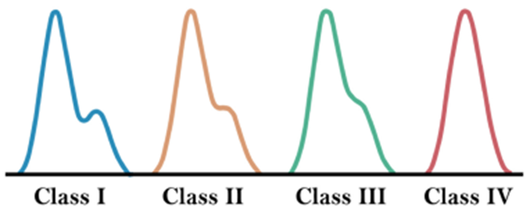
As expected, the speed of the backflow wave increases as vascular beds become stiffer. More delayed arrival of backflow to the aorta in healthy young individuals causes a more pronounced DN. A rushed backward wave, however, reduces the phase difference between the forward and backward flows and, as a result, the DN prominence.
The cardiovascular system is a closed-loop network of multi-branched vessels continuously circulating a complex fluid, blood, using a pulsating pumping organ, the heart. This system is also affected by many concurrent internal/external dynamic actors (e.g., autonomic nervous system, environmental parameters such as temperature, and various noise sources). Hence, the patterns of local flow and pressure signals can be highly complicated and unexpected. Figure 3 shows a small selection of various waveforms that we commonly observe in our in-vivo dataset. Numerous fluctuations and/or vanishing DN morphology are noticeable in these examples. Such complexities must be considered when designing the DN detection approaches to achieve high performance and reliability in edge cases.
Fig. 3.

A few examples of ABP waveforms in the dataset and their expert-annotated DN placement.
3. RELATED WORK
Rule-based and model-based approaches are two general methods previously discussed in the literature for automatic DN detection using ABP/PPG signals.
Rule-based approaches utilize a set of expert-crafted rules to find the DN location. They are the dominant approach in real-time applications because of their speed and simplicity. Li et al. [11] define an empirical method for DN detection with the assumption that two inflation points are present in common blood pressure signals. Then, the first zero crossing following the second inflation point indicates the suggested DN location. Singh et al. [12] propose using a smoothed version of the first derivative to find the major maximum point and thus the DN location on the blood pressure waveform. Chakraborty et al. [13] utilize an empirical formula for DN detection using the first and second derivatives of the denoised PPG signal. They target DN detection in specific low-resource telemonitoring applications where speed and power are limited. To the best of our knowledge, this work is the only method with a PPG dataset including pathological conditions from cardiovascular patients. Balmer et al. [14] focus on locating the end-systolic point in notch-less ABP waveforms derived from distal blood pressure measurements. They use a probabilistic weighting of second derivative peaks to recognize the end of the systolic duration while considering the previous heartbeat results. As common in most derivative-based methods, the performance of rule-based methods is brittle and sensitive to noise and unexpected blood pressure deformations. Thus, a rule-based algorithm may fail to generalize in variant deformation occurrences where the DN detection can be challenging.
Model-based approaches, on the other hand, use the underlying differential equations governing the physiological system to explain the pressure signal and extract the main characteristics of the cardiovascular system including the DN location. The model-based approaches can potentially generalize under unexpected morphology variations as they analyze the underlying physiological system. However, their added complexity and non-convex structure make the optimization convergence sensitive to the optimization methodology and parameter initialization. As a result, their application for DN detection has been limited to close to normal blood-pressure curves where convergence is more easily achievable. Hoeksel et al. [15, 16] utilize a simple three-element Windkessel Model [17] to estimate the arterial blood flow from the input ABP signal. They locate DN to be where the first backflow occurs. Politi et al. [18] studies the effect of vascular resistance on DN shape and location using a numerical model of the vessels with viscoelastic walls. Myers et al. [19] use a four-compartment cardiovascular model and a four-stage optimization algorithm to characterize cardiovascular function. To enhance convergence and performance, their algorithm first prioritizes the five most sensitive parameters during the first two stages, learns the remaining parameters in the third stage, and refines the parameters manually for further improvement in the fourth stage.
In this work, we propose a physics-aware method, PW, that combines the strength of both model-based and rule-based approaches. Our proposed model-based augmentation methodology is designed to consider ABP waveform deformations that have not been covered before. It identifies the common local minima traps and guides the optimizer to convergence during two stages of optimization. The proposed rule-based algorithm is then fine-tuned with the estimated parameters from the model-based step and applied on both ABP and the augmented waveform for final DN placement. To allow application-specific modification, our model-based method can be combined with any user-defined set of rules using a hybrid voting method.
This article is a modification and extension of our previous work [20], where we have proposed the voting DN detection approach (only with pre-existing rule-based algorithms) using a more complex cardiovascular model that has an extra inertance and compliance in the vascular section. The complex model can estimate the ABP patterns more closely and smoothly in comparison to a simple substitute that we use in this article. Thus, it improves the voting accuracy when using a pre-existing rule-based algorithm. Yet the higher complexity of the model makes the optimization less robust and the model prone to instability. In this work, we use a simpler and more stable model in combination with a proposed rule-based algorithm that can compensate for the lower smoothness of the augmented curves and achieve much better performance under waveform deformations.
4. PHYSICS-AWARE APPROACH TO PATTERN RECOGNITION: RATIONALE
When it comes to high-risk healthcare applications, the reliability standard is particularly strict. Any failure in such applications may cause lifelong damages or even lead to death. Real-world healthcare signals may carry various unexpected patterns due to many concurrent dynamic actors that are present inside the system and its environment. Pattern recognition algorithms must be able to account for such variations to achieve the high-reliability standard of the clinical domain.
While rule-based pattern recognition methods commonly yield rigid and brittle algorithms with low reliability, they are popular in many healthcare applications due to their speed and simplicity. Such algorithms may fail to capture the complicated patterns that arise in a dynamic system. As a solution, the identification and elimination of patterns that do not comply with the rule-based assumptions tend to improve the efficacy of the rule-based pattern recognition algorithm. However, this is not a simple task. The natural concurrency of dynamic phenomena in the physical system imposes a wide range of possible patterns on the captured signal. Hence the level and type of required filtering tend to differ even for different parts of the same dataset from the same patient.
Focusing on the DN detection problem, the question that this article tries to answer is “whether one can adopt the well-established physiological knowledge in the field to identify and eliminate such waveform irregularities in a more generalizable way to enhance detection accuracy?”
physics-aware Approach to DN detection: The non-steady nature of the pulsating blood flow in addition to the intricate dynamics of the non-stationary multi-branched vascular network alongside the effect of many concurrent internal/external dynamic actors make the prediction of local flow and pressure signals highly complicated and thus unexpected. On the other hand, the DN gets less and less pronounced, the stiffer the vascular beds become as a matter of age or other underlying conditions. Given the complicated internal/external dynamics and the vanishing DN morphology (Figure 2), filtration of irrelevant effects on pressure signal is not a simple task. As a result, the filtered signal may carry many unexpected deformations that often mislead the rule-based DN detection algorithm. To circumvent this problem, we aim at employing physiological prior knowledge in the field. More specifically, we use a model-based method for data augmentation before rule-based DN detection.
Model-based learning approaches aim at estimating the parameters of an established physiological model of the cardiovascular system, so the estimations of system dynamics match the observed ABP data as closely as possible. The parameters optimizer can also access prior knowledge on parameters’ range and statistics. As limited as such knowledge might be, its incorporation in the learning process helps convergence probability and decreases the required learning time. The resulted model-based approach can identify the relevant simplified patterns and, thus, augment the input signal by eliminating its intractable dynamics. The estimated patterns would be restricted by the boundaries of the defining Ordinary Differential Equations (ODE) model. This way, the estimated signal is explainable and follows the expected behavior. As such a model considers the underlying mathematics that governs the system, the approach can achieve higher generalizability to deal with unexpected scenarios that may arise.
5. PHYSIOWISE: PHYSICS-AWARE DN IDENTIFICATION METHODOLOGY
The details of the proposed physics-aware approach are depicted in Figure 4. The proposed approach can be segmented into four key components, data preprocessing, data augmentation, PW rule-based algorithm, and voting. It is noteworthy that the last two components depict two separate DN estimation methodologies.
Fig. 4.
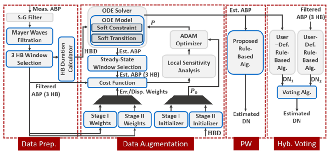
Data preprocessing, data augmentation, and both PW and hybrid voting DN detection procedure block diagram.
Data preprocessing is designed for basic noise reduction of the ABP signal. Then, the signal is divided into 3-heartbeat windows, each being passed to the data augmentation segment separately. During data augmentation, the physiological prior knowledge is employed for extracting the relevant signal patterns and eliminating unrecognized noise effects. Learning parameters of a simplified cardiovascular model (ODE model) to explain the 3-heartbeat input ABP signal, the secondary estimated ABP waveform (output of the ODE solver) would only carry effects that comply with the simplified model mathematics. Thus, the deformation effect is drastically reduced when augmented data is passed to the rule-based method. PW uses the rule-based algorithm proposed in this article. Yet the rules set can be replaced with any other user-defined rule-based DN detection algorithm if required for a specific application.
The preprocessing component (Figure 4) is designed to reduce the signal noise. We use the Savitzky–Golay (S-G) filter [21], a moving average filter to smooth the ABP signal. It was selected due to its advantage of sharpedge preservation [22]. However, as expected, it cannot fully eliminate the effect of many concurrent dynamics affecting the ABP signal.
5.1. Data Preprocessing
The Mayer waves effect (a cyclic change of ABP waveform [23]) is then assumed to be of the form where is the Mayer wave frequency. holds for all the input signals in our dataset. We have identified by fitting a sine wave to diastolic minimum pressures and, then, omitted the effect of the Mayer wave on the signal. We chose to use diastolic minimum points as they are less likely to show extra bumps and deformations while the systolic maximum points can commonly be deformed.
5.2. Cardiovascular Model
Our simplified cardiovascular model is composed of three single-input single-output compartments connected in a closed-loop (Figure 5(a)). These compartments, the left pulsating heart (LPH), arterial systemic compartment (ASC), and post-arterial systemic compartment (PASC), are illustrated in Figure 5. Figure 5(b) shows the ASC and PASC compartments circuitry.
Fig. 5.
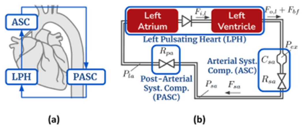
(a) Three-compartment cardiovascular model overview. (b) Cardiovascular circuit model.
P: pressures, R: hydraulic resistances, C: compliances.
In Ursino’s model, the heart’s pumping pulses are modeled as an output flow source with a single squared sinusoidal pulse during the left ventricular ejection time. We have extended the function of , the ventricular output flow source, to include the DN activation function. As discussed in Section 2, the DN is caused by a brief aortic back-flow at the end of systole duration. The effect of aortic back-flow, , is modeled in Equation (1) as a flow source parallel to the and are left ventricle’s blood volume and input blood flow, respectively (detailed equations can be found in Ursino et al. work [24]).
| (1) |
in each heart beat duration is then modeled with a Sine-squared function with magnitude, , duration, , and unset time, , as shown on Equation (2).
| (2) |
The ASC and PASC compartments of the cardiovascular model (Figure 5(b)) can be explained with Equations (3) to (5). In these equations, is the total blood volume. Subscripts , , and denote left ventricle exit region, systemic arteries, post-arterial region, and left atrium, respectively.
| (3) |
| (4) |
| (5) |
To use a gradient-based optimizer, the model needs to be differentiable. Hence, we must approximate and substitute the “unsmooth” components (components that are not differentiable) in the model. Among the different components, we identified two “unsmooth” groups: the components with a non-negativity constraint (i.e., hydraulic compliance, resistance, blood volume, backflow amplitude, and time components) and the components with piece-wise functions (Equation (2) and and equations from baseline model [24]).
For the first group, we used the soft constraint method. In order to ensure the learned parameter is non-negative, a secondary unconstrained parameter is created, where . This way, any function that uses remains smooth and due to the natural positive value of the exponential function , we are guaranteed to have a non-negative .
The second group of unsmooth components are piece-wise functions of the form presented in Equation (6); where is a linear function of the numerical time step, is a sine-squared function of , and is a constant value. To represent the backflow Equation (2) at the numerical time step , we should set , , and .
| (6) |
To work with this group of components, we used the tanh function approximation. The approximation replaces the piece-wise function with , according to Equation (7). is a constant factor defining the slope of transition between −1 and 1 in the tanh function. For large values of , the approximated implementation behaves almost similar to the original piece-wise function with a smoother differentiable transition between 0 and .
| (7) |
5.3. Optimization Methodology
The optimizer’s goal is to minimize the distance between the ODE solver’s output, i.e., estimated ABP waveform, and input signal, i.e., preprocessed ABP waveform, by tuning ODE model parameters. It also aims for recognizing major signal features such as systolic and diastolic pressures, and DN placement.
The non-linear and non-convex structure of the differential equations governing the cardiovascular function (even in its simplified form) makes the parameter optimization step quite challenging. While convergence to global minima will not be guaranteed, the optimizer can get trapped in a local minima that prevents correct DN detection or does not generate a visible DN at all. The cost function, optimizer setting, and parameters’ initialization are major contributing factors that should be systematically tuned to mitigate the problem.
5.3.1. Bayesian Cost Function.
Optimization for a non-convex model can be guided through its cost function. More specifically, the cost function introduces the optimization priorities that can guide the gradient descent algorithm out of unfavorable local minima. We have utilized a Bayesian cost function to tackle the challenge of optimization in the non-linear and non-convex space under study. Such cost functions are designed to use the prior literature-driven knowledge on physiological parameter values to limit the search space of the parameter estimation and improve the convergence.
The proposed Bayesian cost function Equation (8) minimizes the sum of two separate weighted terms. They are the squared error of the estimated pressure and squared parameters displacement at each iteration step .
| (8) |
where , and are estimated parameters vector, parameters average value vector, parameters standard deviation vector, estimated arterial pressure, and measured arterial pressure, respectively. and are the weight vectors of the displacement and error terms.
Squared error term: The error term calculates the weighted sum of the squared distance between the estimated output and the input signal. The optimizer will be penalized more if it misses the most indicative features, namely systolic and diastolic pressures, which have been proven to be of significance in prior literature. Before optimization starts the systolic and diastolic peaks are pinpointed on the measurement curve, and their indices are fed into the cost function’s weight generator ahead of the optimization initiation. To magnify the effect of the systolic and diastolic blood pressures in the cost function, is then increased for a small window around the peaks.
Squared parameter displacement term: The displacement term limits the parameters’ search space by considering the prior average value of the parameters, driven by literature, and an educated guess over the parameters’ standard deviation. The non-convex optimization is guided to convergence by penalizing the cost function with the squared distance between estimated and prior average values of the parameter vector. Similar to the squared error term, the squared parameter displacement term has the ability to highlight the significant parts of its input by increasing their assigned weights. We use this ability to give more displacement freedom to parameters with a higher effect on the estimated signal in comparison to other parameters.
A parameter’s displacement freedom is higher if its standard deviation is higher and thus an overall lower weight is assigned to its displacement term in the cost function. In other words, the optimizer can distance the value of such a parameter from the average at a lower cost. Ideally, these weights must be set using the inverse of the covariance matrix driven by prior knowledge in the field. However, the values are not readily available in case of the cardiovascular modeling. Another solution is to utilize a global sensitivity analysis of the cost function with respect to every model parameter (prior to the estimation process) to find a rough estimation of the covariance matrix. However, the approach is data-driven and case-specific while lacking perspective over the expected physiological parameters’ spread. Also, the cardiovascular model stiffness leads to model instability during global sensitivity analysis under practically unacceptable parameter ranges which are not of concern during the optimization process. Instead, we use an educated guess about the standard deviation terms. The selected variances are provided later in the article.
5.3.2. Transient Response Influence.
As parameters vary, through the estimation process, the convergence from initial values of the state variables to their new steady-state values creates a transient response. In the presence of such a continually-changing transient response, the question is which section of the estimation signal, from initial values to the steady-state response, should be used to compute the cost function. Ideally, the algorithm can learn both the initial values of state variables and the parameters. But this methodology overwhelms the learning algorithm and hinders the convergence in our system. In this article, the estimation process aims to only fit the steady state response of the model to the data. For implementation, we allow a small extra simulation time until the forward ODE solver reaches the steady state. Then the steady state results are fed into the cost function as the estimated signal, .
5.3.3. Optimizer Setting.
The parameter estimator algorithms used in this article are all gradient descent methods. We calculate the gradient of the cost function for each parameter value using a local sensitivity analysis algorithm. The continuous local sensitivity analysis (CSA) method [25] has been selected considering the relatively small number of parameters under optimization (less than 100) and its timing benefits.
The forward-mode of CSA calculates the model sensitivities by extending the ODE system to include Equation (9); where is the Jacobian of the derivative function with respect to the current state variable, , and is the gradient of the derivative function concerning the th parameter.
| (9) |
Hence, the sensitivities are computed to the same error tolerance as the original ODE terms and only a single numerical ODE solver call is required [25].
5.3.4. Optimization Procedure.
To further advance the optimization strategy, we should study the optimization procedure and the effect of each parameter variation on the estimated signal. The optimization results show that the optimizer usually gets trapped in a local minima under various deformations. This is due to the fact that initialization plays a significant role in optimization convergence when dealing with non-convex structures.
To guide the optimizer out of local minima, two significant control knobs are available. Those are displacement freedom weights and initial parameter values. For an effective tuning of such control knobs, a deeper understanding of the optimization procedure and parameters variation effect on the estimated signal is required. We have observed that when initializing parameters with values that are driven from literature (Figure 8(a)), the estimated signal may be distanced far from the measured ABP. The optimizer would then focus on recognizing the outstanding patterns with the highest effect on the cost function, which are usually the main maximum and minimum peaks in the signal. In other words, systolic and diastolic pressures are the first target of the optimization procedure.
Fig. 8.
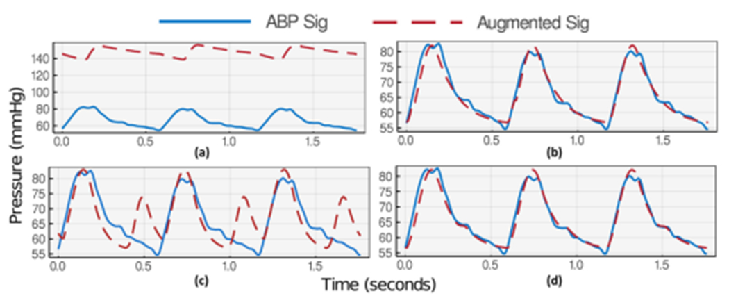
Successful two-stage optimization for the aforementioned example of ABP waveform. (a) First stage initialization. (b) First stage optimization results. (c) Second stage initialization. (d) Second stage optimization results.
To explain the maximum shape and placement, the optimizer employs all tools at hand, including both the main forward pumping flow and the DN backflow. As a result, at the end of the optimization step, the backflow features become false contributing factors to the main systolic peak and, thus, more resistant to variation. During this stage, the common trap is when the optimizer syncs the phases of the forward and backward flows to achieve the highest rising maxima during the systolic peak. Due to unexpected deformations near the systolic peak, the optimizer may also bring the phases closer together to get higher maxima but tune the distance to explain an unwanted deformation near maxima.
First Stage Optimization:
The first stage optimization imitates the general positioning and morphology of the blood pressure curve. At the same time, the cost function displacement term keeps the parameters in the expected physiological range. Therefore, at the beginning of the first stage, the parameters are initialized to their average values , derived from clinical literature [24]. For parameters with no prior expected values, we have picked the initial values based on the optimizer’s stability through several algorithms runs. Table 1 lists the initialization of the parameters for the first stage. Commonly there is no visible DN placement on the estimated ABP waveform at the end of the first optimization run. Since the initial placement and shape of the estimated signal are much distanced from the output signal, the optimizer tries to learn the pattern of outstanding features in the output signal, namely main peaks. To achieve that, it usually optimizes the parameters to get a similar phase on systolic and DN bumps or silences the DN bump in a far-off placement. Therefore, the optimizer is commonly trapped in a local minima at this point and cannot find a way out. To prevent backflow contribution to the systolic peak, we have manually silenced the DN parameters and restrained their variation freedom during this step. Thus, similar to the actual cardiovascular system behavior, the optimizer focuses on finding the systolic maxima and diastolic minima only using the main pumping flow and other systemic parameters. The optimization results at the end of the first stage are depicted in the Results section, Figure 8, part (b).
Table 1.
Stage I: Parameters Initialization
| Average values driven from [24] and the assigned standard deviations | ||
|---|---|---|
| Compliance , | Hydraulic Resistance (), | Volume |
|
|
||
| Problem-specific initial values and standard deviations | ||||
|---|---|---|---|---|
| Pressure, | Flow, | Volume, | Time, | Amplitude |
|
|
|
|||
| – | – | – | ||
Second Stage Optimization:
During the second stage initialization, the estimated parameters from the first stage optimization are altered to magnify the expected DN location in the estimated waveform. A high DN peak is imposed on the previously estimated arterial pressure in stage one using the expected average DN placement. The parameter displacement freedoms are also set to give freedom to changing backflow parameters while restraining all other parameters learned during the last stage. As a result, the optimizer is guided out of the local minima to focus on DN shape and location during the second-stage parameter estimation. The case-sensitive parameter alteration Equation (10) is applied to the backflow parameters to adjust the DN shape and location. The value of is also divided by half to increase the downward diastolic slope. This slope is commonly excessively flattened during first stage optimization to compensate for dicrotic or other deformation bumps on the signal.
| (10) |
| (11) |
where is the heart-beat time period.
The second stage initialization and optimization results are shown in the Results section in Figure 8 parts (c) and (d), respectively. The final estimated ABP waveform at the end of the second stage optimization visualizes a clear-cut DN identification.
5.4. Proposed Rule-based Algorithm
Our proposed rule-based algorithm extends Li et al. [26] proposed rule-based method to account for inputs from the model-based step. Li finds the DN placement by limiting the search window on the ABP waveform using some simple preset rules based on the distance from systolic and diastolic peaks. Within each search window, the algorithm looks for the first zero-crossing point on the first derivative curve. If no zero-crossing points exist in the search window, the algorithm finds the first empirical point as the DN placement. This method is highly dependent on the search window selection and the noise of the dataset. Zero-crossing points are pretty common in a deformed ABP waveform which has been misleading Li’s algorithm when applied to our dataset.
The fluctuation of model-based augmentation of the original ABP signal is much smoother under the limitations of defined ODEs. These fluctuation patterns meet the physiological prior knowledge to highlight DN location on a deformed waveform. The learned parameters of the augmented model can approximate the expected range of DN placement on both ABP and its augmented curve. Such input can enhance the accuracy of DN placement while simplifying the required rules.
Instead of using distance from peaks, PW overwrites the search window using the learned parameters of the model-based augmentation. Also, it uses the augmented and thus smoother version of the waveform when finding DN placement. Equations (13) to (14) show the set of PW rules that overwrite the lower and upper limits of the search window, and , if overwrite condition is met for heartbeat , and denote the pulse start time, systolic peak time, transmission time, and marginal time respectively.
| (12) |
| (13) |
| (14) |
5.5. Voting Procedure
The PW approach does not require voting if the proposed rule-based algorithm is used. However, if one wishes to use a hybrid modality with another rule-based method of choice for a specific application, voting can combine the proposed model-based technique in this article and the selected rule-based method to gain higher performance. In such a scenario, the proposed model-based approach is first applied to the ABP data to estimate the augmented version. Next, both the augmented curve and ABP curve are scanned by the selected rule-based algorithm for DN placement. The voting method then receives both result sets and compares the DN placements to identify the DN location. During the voting procedure, if both rule-based and hybrid algorithms have placed a DN location for a heartbeat, the average position is identified as the voting result. Otherwise, if one failed to find a DN location in a heartbeat under study, the result of the other algorithm decides the DN position.
6. RESULTS
We have implemented the cardiovascular model and the parameter estimator using the Julia Language [27–30].
6.1. Dataset
We have analyzed ABP signals for 24 datasets randomly selected from 4 and 10 pigs undergoing sepsis and hemorrhage recovery studies, respectively, for our experimental demonstration. The studied pigs are all administered bolus therapy with a rate of 100ml/s in continuous ejection and rest time windows of 60s. For the sepsis experiments, the ABP was measured using a 5-French intra-arterial sheath placed into the carotid artery. For the hemorrhage animals, the ABP was measured using a 7-French catheter that was inserted into the carotid artery that was threaded into the proximal aorta. More details about the study can be found in [31]. Data acquisition is also done using the PowerLab device [32].
Each random dataset contains 27 heartbeats and there are 648 heartbeats in total. All the DNs are manually annotated by an expert physician. These annotations are the gold standard against which the performance will be compared. The dataset sampling frequency is 100 Hz. We went through the preprocessing method explained in Section 5.1 to remove noise and other artifacts from the raw signal as shown in Figure 6.
Fig. 6.
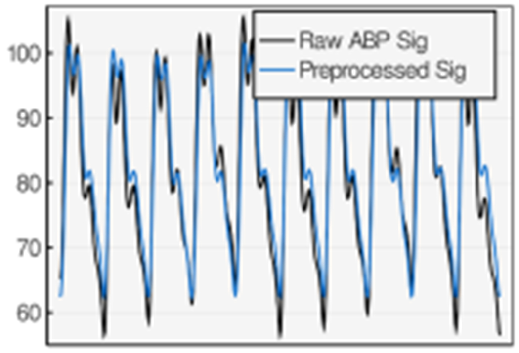
The ABP signal before and after preprocessing step.
6.2. Evaluation Metrics
We define the error of DN detection in each heartbeat time-series, , to be the absolute time difference between the gold-standard and detected DN location in each heartbeat Equation (15).
| (15) |
Using the aforementioned heartbeat-level definition of , Equation (16) presents the defined DN detection accuracy percentage, , in a dataset, , containing a vector of heartbeats, , under a maximum permitted error, .
| (16) |
where stands for the cardinality of set .
6.3. Hyperparameter Tuning
For the optimizer algorithm, we have selected the Adam optimizer [33] for its adaptive parameter tuning (with respect to each parameter’s past update history) and momentum consideration that can lead to a shorter run time.
We have preset the ADAM optimizer learning rate equal to 0.01 and the first and second decay of momentums equal to 0.9 and 0.999 consecutively.
The results of the proposed optimization methodology demonstrate effective guidance of cost function outside unfavorable local minima. To support the choice of three heartbeats per optimization, we have included the failed optimization results of a single heartbeat window for an example of an ABP waveform (Figure 7). Figure 8 then shows how the proposed optimization algorithm can recognize the DN pattern in the same example when using a three heartbeat window.
Fig. 7.
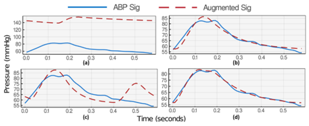
Failed two-stage optimization algorithm progress in an example of ABP waveform when considering only a single heartbeat. (a) First stage initialization. (b) First stage optimization results. (c) Second stage initialization. (d) Second stage optimization results.
Figures 7(a) and 8(a) each shows a snapshot of the first stage initialization with values summarized in Table 1. During this optimization stage, we have identified , and as the most effective parameters for signal position and swing. Thus, we have assigned a lower displacement weight of 0.1 to them while all other parameters’ displacement weight is set to 10. To guide the optimizer to focus on systolic and diastolic pattern recognition, is set to 5 for indices with distance from maximum and minimum and 1 for all other indices. The results of the first stage optimization (Figures 7(b) and 8(b)) depict a successful learning of systolic and diastolic pressures (maximum and minimum) using both window selections.
Then, initializing the parameters for the second stage optimization in Figures 7(c) and 8(c) creates an exaggerated DN maxima. At this stage of optimization, the most effective parameters on DN shape and position are , and . These parameters’ displacement term is, thus, set to 10 while keeping other parameters constant. term is also reset to 1 for all indices including maximum and minimum range as their learning is not the attention of this stage of optimization. The final results show successful visual DN recognition in Figure 8(d) for the three-heartbeat window, while the single-heartbeat window choice in Figure 7(d) shows no upstroke (no DN) on the descending part of the estimated wave and gets trapped in the local minima. Such behavior is commonplace based on many results we have gathered. Intuitively, having more heartbeats during optimization provides a better understanding of the parameters’ effect on the signal and reduces the chance of overfitting to a small and limited feature window.
6.4. DN Detection Statistics
We have first tested our hybrid approach with two pre-existing rule-based methods [26, 34]. Alexander Laurin developed the rule-based DN detection algorithm using the technique of derivatives and thresholds described by Pan et al. in [34]. Li et al. [26] proposed an automatic delineator for the fiducial points of ABP waveforms, namely their onsets, systolic peaks, and DN. From this point forward we use the following acronyms for different combinations of methods. LRB and PRB are Li’s and Pan’s vanilla rule-based algorithms. LHyb and PHyb denote the hybrid method before voting where Li’s and Pan’s rule-based algorithms are applied to the augmented waveforms. LVot and PVot are the hybrid voting method using Li’s and Pan’s pre-existing rule-based algorithms. PW, as mentioned before, would be the PW physics-aware approach where the proposed rule-based algorithm is applied to the augmented data without voting.
We present the DN detection results on two datasets in Figure 9 as example plots. The depicted results compare the DN detected using pure rule-based, hybrid, voting, and PW approaches with expert-annotated golden DN locations. While the proposed method shows much more reliable results in many cases of ABP deformations, the rule-based algorithm fails to recognize the DN position on the augmented signal in some others. As derivative-based rules are sensitive to noise and unexpected deformations, they might fail to capture the DN due to slight pattern modification. This issue is even worse with second derivatives. A voting mechanism improves the statistics of locating DN in such failed cases.
Fig. 9.
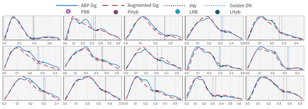
A diverse example of augmentation and DN placement results. All augmented waveforms are estimated using three consecutive ABP pulses, yet only the first pulse is shown for simplicity.
Table 2 provides statistics of DN detection quality under different methods. The results show that the hybrid approach with voting can improve the mean error by 17% while reducing its standard deviation by 25%. The Table provides the statistics of best and worst per dataset cases of DN detection where is set to be 30ms (the strict permitted error range), 50ms (typical permitted error range), and 70ms (tolerant permitted error range). Focusing on the typical error range setting, the results show up to 67% accuracy improvement in the best case with only a −14% decline in the worst case. The last row of Table 2 shows the PW results. As explained before, PW uses a model-based approach and the proposed rule-based algorithm (no voting step) to find the DN placement. We have also used and when implementing Equations (13) to (14). The results suggest 52% and 54% lower error and standard deviation in comparison to the best results of tested pre-existing rule-based methods. PW also shows 16% higher accuracy in the permitted error range of 30ms.
Table 2.
DN Detection Statistics under Different Methods
| Overall Err statistics | , | , | , | ||||||||
|---|---|---|---|---|---|---|---|---|---|---|---|
|
| |||||||||||
| Method | Mean, (ms) | SD, (ms) | Total | Best Dset improv. | Worst Dset improv. | Total | Best Dset improv. | Worst Dset improv. | Total | Best Dset improv. | Worst Dset improv. |
| LRB [26] | 49 | 37 | 41% | – | – | 63% | – | – | 78% | – | – |
| LHyb | 50 | 46 | 40% | 37% | −55% | 59% | 48% | −53% | 76% | 52% | −46% |
| LVot | 40 | 44 | 43% | 19% | −57% | 67% | 40% | −23% | 84% | 33% | 0% |
|
| |||||||||||
| PRB [34] | 42 | 61 | 68% | – | – | 86% | – | – | 86% | – | – |
| PHyb | 48 | 62 | 56% | 55% | −77% | 72% | 55% | −55% | 89% | 74% | −29% |
| PVot | 35 | 46 | 66% | 37% | −59% | 87% | 67% | −14% | 91% | 76% | −7% |
|
| |||||||||||
| PW | 20 | 28 | 82% | – | – | 89% | – | – | 90% | – | – |
6.5. Discussion
Figure 10 shows the Bland–Altman comparison of LRB algorithm with three methods. The comparison with LHyb is depicted in Figure 10(a). This plot shows a poor agreement between the rule-based and hybrid methods.
Fig. 10.

Bland–Altman comparison of DN placements using input method 1, LRB, and (a) LHyb method as input method 2. (b) LVot method as input method 2. (c) PW as input method 2.
LVot method is compared with LRB method in Figure 10(b), where a slightly higher agreement is observable. This plot also suggests that LVot commonly estimates higher DN placement in the low-value segment of LRB results, while estimating lower DN placement for high-value results. Figure 10(c) shows the comparison with PW input method where PW is leaning towards estimating larger values than LRB algorithm with an average difference of 37ms. While the overall agreement is lower on this subplot, a stronger agreement than previous methods is observable for mid-range values.
We have done a similar Bland–Altman comparison for PRB algorithm and three methods on Figure 11. The PHyb approach shows much higher agreement with PRB method (Figure 11(a)) in comparison to the first comparison in Figure 10(a). As expected, the agreement is boosted in Figure 11(b) when using PVot method. Based on these results, Pan’s method seems to generate larger DN placement estimates in comparison to Li’s method. Thus a slightly higher correlation is observable between PW approach and the PRB algorithms as shown in Figure 11(c).
Fig. 11.

Bland-Altman comparison of DN placements using input method 1, PRB, and (a) PHyb method as input method 2. (b) PVot method as input method 2. (c) PW as input method 2.
In this article, we consider hard datasets for a specific rule-based algorithm to be the ones with an under . In other words, a dataset is hard for a rule-based algorithm if the algorithm cannot find the DN location of more than 50% of its heartbeats with .
The DN detection evaluation of 24 datasets finds 10 and 3 hard cases for Li’s [26] and Pan’s [34]. We then select three hard cases for each rule-based algorithm and apply our proposed DN detection approaches to test the accuracy level for a varying . As shown in Figures 12(a) and 13(a), PW and the hybrid voting methods can achieve superior performance on real-world ABP signals prone to noise and artifacts.
Fig. 12.
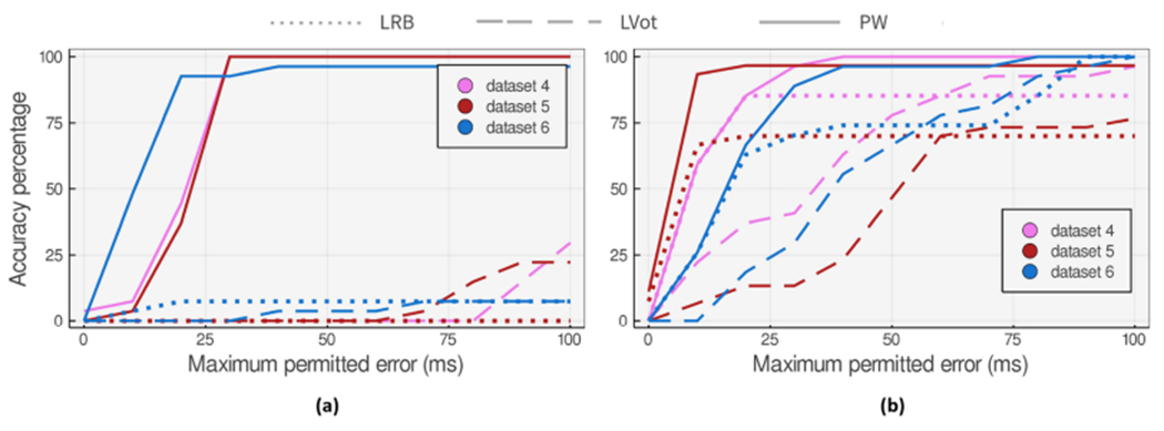
Accuracy of the proposed DN detection approaches applied to 27 heartbeat datasets that (a) are hard cases for LRB method. (b) show the worst accuracy degradation at in comparison to LRB method.
Fig. 13.
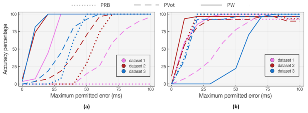
Accuracy of the proposed DN detection approaches applied to 27 heartbeat datasets that (a) are hard cases for PRB method. (b) show the worst accuracy degradation at in comparison to PRB method.
We also studied the three worst accuracy degradation cases (at ) when applying the voting method to Li’s and Pan’s algorithms. Figures 12(b) and 13(b) show the accuracy comparison of the methods applied to these cases for a varying maximum permitted error.
Our study on the hybrid approach shows that even when DN is visually detectable on the augmented waveform, the high sensitivity of pre-existing rule-based algorithms to unexpected changes might mislead the hybrid algorithm and lower the overall accuracy. We have proposed the voting method to mitigate the issue in cases where the pre-existing rule-based algorithm fails to correctly detect DN on the augmented signal but returns better results with the ABP waveform. Although voting improves the accuracy, fine-tuning the user-defined rule-based method to capture the patterns of the augmented signal seems essential.
Using the PW and its proposed rule-based algorithm, we can commonly find DN locations more accurately or closely comparable to the pre-existing rule-based algorithm. There are also a few cases of vanishing DN like dataset 6 on Figure 13(b) that PW does not show acceptable performance on. Although we see a comparable performance from PW on some data points with vanishing DN, there are some examples where the model-based algorithm fails to highlight the DN location correctly when DN is much less pronounced. There are a few cases of Class IV ABP waveforms (refer to Figure 2) in the dataset (less than 5% of the whole samples) where DN is not visible and the downward ABP shape is a smooth concave curve. Yet the authors do not claim better performance in such scenarios.
7. CONCLUSION
In this work, we have proposed a physics-aware methodology with a generalizable DN detection capability in the presence of many typical blood pressure curve deformations and mild cases of vanishing DN morphologies. The method has shown a 52% mean error improvement on real-world expert-annotated pig data undergoing sepsis and hemorrhage study. However, more study needs to be done on the possibility of fine-tuning the optimization technique or using other time-series measurements to locate DN in severe vanishing cases where DN is very subtle or invisible. Although it is out of the scope of this article, a more in-depth study of the speed limitations of model-based methods can help with extending their usage to also cover the time-constrained target applications where the restrictions can be met.
CCS Concepts:
• Applied computing → Systems biology; • Theory of computation → Nonconvex optimization;
Acknowledgments
This work was supported by the National Science Foundation (NSF) Grant No. IIS-1838939, NSF award 1937158, the National Institutes of Health (NIH) award R21HD097467, and Department of Defense (DoD) CDMRP Grant No. W81XWH1820072.
J. Y. Adams is a co-founder of Certus Critical Care Inc., a company working to develop rule-based and machine learning approaches to automating aspects of critical care.
Contributor Information
MAHYA SAFFARPOUR, Department of Electrical and Computer Engineering, UC Davis.
DEBRAJ BASU, Department of Electrical and Computer Engineering, UC Davis.
FATEMEH RADAEI, Department of Electrical and Computer Engineering, UC Davis.
KOUROSH VALI, Department of Electrical and Computer Engineering, UC Davis.
JASON Y. ADAMS, Department of Pulmonary and Critical Care Medicine, UC Davis School of Medicine
CHEN-NEE CHUAH, Department of Electrical and Computer Engineering, UC Davis.
SOHEIL GHIASI, Department of Electrical and Computer Engineering, UC Davis.
REFERENCES
- [1].Lehman Li-wei H, Ryan P. Adams, Mayaud Louis, Moody George B., Malhotra Atul, Mark Roger G., and Nemati Shamim. 2014. A physiological time series dynamics-based approach to patient monitoring and outcome prediction. IEEE Journal of Biomedical and Health Informatics 19, 3 (2014), 1068–1076. [DOI] [PMC free article] [PubMed] [Google Scholar]
- [2].Jozwiak Mathieu, Monnet Xavier, and Teboul Jean-Louis. 2018. Pressure waveform analysis. Anesthesia and Analgesia 126, 6 (2018), 1930–1933. [DOI] [PubMed] [Google Scholar]
- [3].Maheshwari Kamal, Buddi Sai, Jian Zhongping, Settels Jos, Shimada Tetsuya, Cohen Barak, Sessler Daniel I., and Hatib Feras. 2021. Performance of the Hypotension Prediction Index with non-invasive arterial pressure waveforms in non-cardiac surgical patients. Journal of Clinical Monitoring and Computing 37, 1 (2021), 71–78. [DOI] [PMC free article] [PubMed] [Google Scholar]
- [4].Pickett Joya D., Bridges Elizabeth, Kritek Patricia A., and Whitney JoAnne D.. 2018. Noninvasive blood pressure monitoring and prediction of fluid responsiveness to passive leg raising. American Journal of Critical Care 27, 3 (2018), 228–237. [DOI] [PubMed] [Google Scholar]
- [5].Guyton Arthur and Hall John. 2006. Textbook of Medical Physiology, Saunders Co. (2006). [Google Scholar]
- [6].Lewis Richard P., Rittogers SE, Froester WF, and HARIsIOs Boudoulas. 1977. A critical review of the systolic time intervals. Circulation 56, 2 (1977), 146–158. [DOI] [PubMed] [Google Scholar]
- [7].Biering-Sørensen Tor, Roca Gabriela Querejeta, Hegde Sheila M., Shah Amil M., Claggett Brian, Mosley Thomas H. Jr, Butler Kenneth R. Jr, and Solomon Scott D.. 2018. Left ventricular ejection time is an independent predictor of incident heart failure in a communitybased cohort. European Journal of Heart Failure 20, 7 (2018), 1106–1114. [DOI] [PMC free article] [PubMed] [Google Scholar]
- [8].Dawber Thomas R., Thomas H. Emerson Jr, and McNamara Patricia M.. 1973. Characteristics of the dicrotic notch of the arterial pulse wave in coronary heart disease. Angiology 24, 4 (1973), 244–255. [DOI] [PubMed] [Google Scholar]
- [9].Millasseau Sandrine C., Ritter James M., Takazawa Kenji, and Chowienczyk Philip J.. 2006. Contour analysis of the photoplethysmographic pulse measured at the finger. Journal of Hypertension 24, 8 (2006), 1449–1456. [DOI] [PubMed] [Google Scholar]
- [10].Tigges Timo, Music Zenit, Pielmus Alexandru, Klum Michael, Feldheiser Aarne, Hunsicker Oliver, and Orglmeister Reinhold. 2016. Classification of morphologic changes in photoplethysmographic waveforms. Current Directions in Biomedical Engineering 2, 1 (2016), 203–207. [Google Scholar]
- [11].Li Bing Nan, Dong Ming Chui, and Vai Mang I.. 2010. On an automatic delineator for arterial blood pressure waveforms. Biomedical Signal Processing and Control 5, 1 (2010), 76–81. [Google Scholar]
- [12].Singh Omkar and Sunkaria Ramesh Kumar. 2017. Detection of onset, systolic peak and dicrotic notch in arterial blood pressure pulses. Measurement and Control 50, 7–8 (2017), 170–176. [Google Scholar]
- [13].Chakraborty Abhishek, Sadhukhan Deboleena, and Mitra Madhuchhanda. 2021. Accurate detection of dicrotic notch from PPG signal for telemonitoring applications. International Journal of Biomedical Engineering and Technology 37, 2 (2021), 121–137. [Google Scholar]
- [14].Balmer Joel, Smith Rachel, Pretty Christopher G., Desaive Thomas, Shaw Geoff M., and Chase J. Geoffrey. 2020. Accurate end systole detection in dicrotic notch-less arterial pressure waveforms. Journal of Clinical Monitoring and Computing 35, 1 (2021), 79–88. [DOI] [PubMed] [Google Scholar]
- [15].Hoeksel SAAP, Jansen JRC, Blom JA, and Schreuder Johannes Jacobus. 1997. Detection of dicrotic notch in arterial pressure signals. Journal of Clinical Monitoring 13, 5 (1997), 309–316. [DOI] [PubMed] [Google Scholar]
- [16].Donelli Andrea, Jansen Jos R. C., Hoeksel Bas, Pedeferri Paolo, Hanania Ramzi, Bovelander Jan, Maisano Francesco, Castiglioni Alessandro, Alfieri Ottavio, and Schreuder Jan J.. 2002. Performance of a real-time dicrotic notch detection and prediction algorithm in arrhythmic human aortic pressure signals. Journal of Clinical Monitoring and Computing 17, 3 (2002), 181–185. [DOI] [PubMed] [Google Scholar]
- [17].Frank O. 1990. Die Grundform des Arteriellen Pulses (translated by Sagawa K, Lie RK, Schaefer J, 1990, J Mol Cell Cardiol 22: 253–277). [DOI] [PubMed] [Google Scholar]; Journal of Molecular and Cellular Cardiology 22, 3 (1990), 253–254. [DOI] [PubMed] [Google Scholar]
- [18].Politi María Teresa, Ghigo Arthur, Juan Manuel Fernández Ismaïl Khelifa, Gaudric Julien, Fullana José María, and Lagrée Pierre-Yves. 2016. The dicrotic notch analyzed by a numerical model. Computers in Biology and Medicine 72 (2016), 54–64. [DOI] [PubMed] [Google Scholar]
- [19].Myers TG, Ripoll Vicent Ribas, de Tejada Cuenca Anna Sáez, Mitchell Sarah L., and McGuinness Mark J.. 2017. Modelling the cardiovascular system for assessing the blood pressure curve. Mathematics-in-industry Case Studies 8, 1 (2017), 1–16. [DOI] [PMC free article] [PubMed] [Google Scholar]
- [20].Saffarpour Mahya, Basu Debraj, Radaei Fatemeh, Vali Kourosh, Adams Jason Y., Chuah Chen-Nee, and Ghiasi Soheil. 2021. Dicrotic notch identification: A generalizable hybrid approach under arterial blood pressure (ABP) curve deformations. In Proceedings of the 2021 43rd Annual International Conference of the IEEE Engineering in Medicine and Biology Society. IEEE, 4424–4427. [DOI] [PubMed] [Google Scholar]
- [21].Schafer RW. 2011. What is a savitzky-golay filter? [Lecture Notes]. IEEE Signal Processing Magazine 28, 4 (2011), 111–117. DOI: 10.1109/MSP.2011.941097 [DOI] [Google Scholar]
- [22].Schafer Ronald W.. 2011. On the frequency-domain properties of Savitzky-Golay filters. In Proceedings of the 2011 Digital Signal Processing and Signal Processing Education Meeting. 54–59. DOI: 10.1109/DSP-SPE.2011.5739186 [DOI] [Google Scholar]
- [23].Julien Claude. 2006. The enigma of Mayer waves: Facts and models. Cardiovascular Research 70, 1 (2006), 12–21. [DOI] [PubMed] [Google Scholar]
- [24].Ursino Mauro. 1998. Interaction between carotid baroregulation and the pulsating heart: A mathematical model. American Journal of Physiology-Heart and Circulatory Physiology 275, 5 (1998), H1733–H1747. [DOI] [PubMed] [Google Scholar]
- [25].Ma Yingbo, Dixit Vaibhav, Innes Michael J., Guo Xingjian, and Rackauckas Chris. 2021. A comparison of automatic differentiation and continuous sensitivity analysis for derivatives of differential equation solutions. IEEE High Performance Extreme Computing Conference (HPEC’21). 1–9. [Google Scholar]
- [26].Bing Nan Li, Ming Chui Dong, and Vai Mang I.. 2010. On an automatic delineator for arterial blood pressure waveforms. Biomedical Signal Processing and Control 5, 1 (2010), 76–81. DOI: 10.1016/j.bspc.2009.06.002 [DOI] [Google Scholar]
- [27].Innes Michael, Saba Elliot, Fischer Keno, Gandhi Dhairya, Rudilosso Marco Concetto, Joy Neethu Mariya, Karmali Tejan, Pal Avik, and Shah Viral. 2018. Fashionable modelling with flux. arXiv preprint arXiv:1811.01457 (2018). [Google Scholar]
- [28].Rackauckas Christopher and Nie Qing. 2017. Adaptive methods for stochastic differential equations via natural embeddings and rejection sampling with memory. Discrete and Continuous Dynamical Systems. Series B 22, 7 (2017), 2731. [DOI] [PMC free article] [PubMed] [Google Scholar]
- [29].Innes Mike. 2018. Flux: Elegant machine learning with Julia. Journal of Open Source Software 3, 25 (2018), 602. DOI: 10.21105/joss.00602 [DOI] [Google Scholar]
- [30].Rackauckas Christopher and Nie Qing. 2017. Differentialequations. jl–a performant and feature-rich ecosystem for solving differential equations in julia. Journal of Open Research Software 5, 1 (2017), 15. [Google Scholar]
- [31].Radaei Fatemeh. 2020. Prediction of fluid-responsiveness in patients at intensive care unit using machine learning modeling. M.S. Plan-I Thesis (2020). [Google Scholar]
- [32].PowerLab. 2021. M.S. Plan-I Thesis, University of California, Davis. Retrieved from https://www.adinstruments.com/products/powerlabdaq-hardware. [Google Scholar]
- [33].Kingma Diederik P. and Ba Jimmy. 2014. Adam: A method for stochastic optimization. arXiv preprint arXiv:1412.6980, (2014). [Google Scholar]
- [34].Pan J and Tompkins WJ. 1985. A real-time QRS detection algorithm. IEEE Transactions on Biomedical Engineering BME-32, 3 (1985), 230–236. DOI: 10.1109/TBME.1985.325532 [DOI] [PubMed] [Google Scholar]


