A Kinetostatic Model for Concentric Push-Pull Robots

Abstract

Concentric push-pull robots (CPPR) operate through the mechanical interactions of concentrically nested, laser-cut tubes with offset stiffness centers. The distal tips of the tubes are attached to each other, and relative displacement of the tube bases generates bending in the CPPR. Previous CPPR kinematic models assumed two tubes, planar shapes, no torsion, and no external loads. In this paper, we develop a new, more general CPPR model accounting for any number of tubes, describing their variable-curvature 3D shape when actuated, including the effects of torsion and external loads. To accomplish this, we employ a modified Kirchhoff rod model for each tube (with offset stiffness center) and embed the constraints of concentricity. We use an energy method to determine robot shape as a function of actuation and external loading. We experimentally validate this kinetostatic model on prototype CPPRs with two tubes and three tubes and non-constant laser-cut patterns that create variable curvature and stiffness. Experimental results agree with the model, paving the way for use of this model in design optimization, planning, and control of CPPRs.

I. Introduction

Concentric push-pull robots (CPPR) are continuum manipulator that consist of concentrically nested tubes, each of which is laser cut with an asymmetric pattern, and the tips of which are fixed together at their distal ends as shown in Figure 1. Relative translations of the tubes generate bending in the overall CPPR structure, while the entire collection can be additionally rotated and translated axially as a group. Such asymmetrically patterned tube actuators have been studied over the past few years, demonstrating constant-curvature modeling, ex-vivo tissue resection, variable curvature kinematic design, and workspace optimization [1]–[3]. They can be fabricated using a number of different methods, including laser machining [1], [4]–[7], conventional milling [8]–[10], and 3D printing [2], [1].

Fig. 1.

Actuation concept and construction of CPPRs. (a) Two or more tubes are laser patterned to create offset stiffness centers. (b) The collection of tubes is nested concentrically, and the tube tips are fixed to each other at their distal ends. (c) Bending actuation is achieved by relative translations of the tubes. (d) A 3 DOF workspace can be achieved for a two-pair CPPR by including collective rotations and insertions of both tubes.

The actuation tubes in a CPPR can carry both tension and extension, enabling active bending in the positive and negative directions through relative translation (i.e. pushing and pulling) of the tubes (in contrast to conventional uni-directional pull-wire actuation). Using thin-walled tubes also enables a large inner lumen space for passing through surgical tools such as grippers, cameras, and illumination. The multi-tube structure also increases the overall stiffness of the manipulator, enhancing its strength and capabilities for load-bearing surgical tasks such as tissue traction. Additional sets of push-pull tubes can also be deployed through the inner lumen of a first set of tubes to further increase the degrees of freedom (DOF) by adding more independent bending segments in series. An example of this is shown in the attached video and Figure 2.

Fig. 2.

Dual CPPR system, consisting of a larger proximal CPPR and a smaller distal CPPR that is housed within the proximal CPPR (a). Using two two-tube CPPRs, 5-DOF can be controlled (b).

CPPRs are similar to pre-curved concentric tube robots (known as CTRs) in some ways. They are both constructed from concentric tubes, have an open inner lumen, can be fabricated at millimeter scales and are capable of traversing complex and tortuous pathways, making them suitable manipulators for minimally invasive surgery (MIS) applications [11]. However, Table I summarizes the main differences. Unlike most CTR designs, CPPRs can achieve a fully straight configuration, and do so trivially. They are less stiff because of the selective material removal, but are consequently able to achieve a wider range of curvatures without hitting strain limits. The maximum degrees of freedom available per tube is slightly less because the tips are attached together. However, the elastic instabilities experienced by CTRs (e.g. [12], [13]) are not present in CPPRs. Thus, while the torsional instabilities of CTRs strongly limits their ability to be actuated remotely over lengthy transmissions, CPPRs are less limited and can be deployed through longer flexible endoscopes. Thus CTRs and CPPRs are lend themselves to different surgical applications. CTRs are more suited to procedures that require higher stiffness and shorter transmission lengths. This facilitates urological surgeries such as uterine dissection and prostate tissue resection. CPPRs are better positioned as dexterous wrists, devices for precise aiming of lasers, and soft tissue manipulation through longer flexible endoscopic channels.

TABLE I.

Comparison of Characteristics Between Cpprs and Ctrs

	CTR	CPPR
Ability to Fully Straighten	In Special Cases	Always
Passive Stiffness	Higher	Lower
Curvature Range	Lower	Higher
Degrees of Freedom	max 2 per tube $\text{(}2n\text{)}$	max 3 per tube pair $\text{(}1.5n\text{)}$
Elastic Stability	Design Dependent	Stable
Remote Actuation	Often Limited by Torsion	Less Limited

In previous research, CPPRs were made with large rectangular notches cut out of the tubes [2], [3], and a constant-curvature beam model was used to describe the bending in the notched sections to create a forward kinematics model for CPPRs [1]. The parameters of the design (the spacing and size of the rectangular notches) dictate the overall bending shape of the CPPR when actuated, and inverse design can be performed [1]. However, this existing work is limited to large rectangular notches, planar actuated shapes, pairs of tubes (not more than two attached together), torsionless configurations, and scenarios without external loads.

Instead of large rectangular notches, CPPRs can also be made with very narrow interleaved slots (on the order of 50–150 microns wide) or even more exotic patterns [14]. The “small slot” paradigm can improve desired structural properties such as torsional rigidity and helps to eliminate any mechanical interference, pinching hazards, and localized buckling that can occur with large notches, but it necessitates a more continuous modeling approach, such as elastic rod theory. In addition, we would like to be able to model scenarios in which CPPRs apply forces to tissue (tumor resection has already been demonstrated in ex vivo models [3]), and to explore new design possibilities such as using more than two tubes attached at their tips to enable more degrees of freedom.

A. Related Modeling Work

Mechanics models such as Kirchhoff rod and Cosserat rod models have been used to create kinetostatic models (i.e. kinematics and statics) for many continuum robot designs. This modeling paradigm has been used to accurately model tendon-driven continuum robots [15]–[18], CTRs [12], [19]–[22], parallel continuum robots [23], [24], fluid-actuated continuum robots [25], [26] and new eccentric tube robots [27], [28]. Kinetostatic models are useful in that the kinematics can be efficiently computed [24] and can capture external loading and arbitrary numbers of tubes and rods. Energy methods related to our approach have also been used on tendon-driven [15], concentric tube [29], and parallel continuum robots [30], [31].

However, the CPPR actuation paradigm presents a challenge that previous models do not account for, namely that the stiffness center of an asymmetrically patterned tube is not coincident with the geometric center of the tube. This complicates the description and enforcement of multi-tube concentricity constraints because the individual tube reference frames are offset from one another instead of coincident.

B. Organization and Contributions

Our contribution in this paper is to derive and experimentally validate a new general CPPR kinetostatic model that overcomes the above challenge of offset stiffness centers in a concentric tube collection and accounts for external loading, general slot cut patterns with variable stiffness, 3D bending and torsion, and any number of tubes. Each tube is modeled as a classical Kirchhoff rod with an offset stiffness center, and constraints of concentricity are derived and embedded in the model. A series of polynomial basis functions at the curvature level is then used to parameterize the configuration of the tube collection. The coefficients of this polynomial series are then found via energy minimization (accounting for external loads) and used to construct the tube shapes and robot pose.

Section II details the derivation of our energy-based kinematics-statics model, beginning with the derivation of the kinematics of a single tube constrained to a centerline and ending with the implementation of the full kinematic model. Section III details an example design of a narrow laser cut slot pattern that offsets the stiffness center of the tubes and demonstrates our FEA-based parameter characterization process for estimating the mechanical properties of the tubes, which are parameters of the model. Section IV covers our experimental validation of the full model, in which we compare model kinematics and loaded deflection predictions with experimental prototypes. We investigate three relevant CPPR design cases: (1) a two-tube, constant-curvature CPPR where the stiffness centers of each tube run parallel with the centerline, (2) a two-tube, ‘converging’ CPPR in which the stiffness centers taper toward the center of the tube down the length, and (3) a three-tube CPPR that can achieve 3D translational positioning of the tip without rotating the tubes. Section V discusses future work and Section VI concludes with a discussion on our validation results. The work in this paper is based on Chapter 4 of the first author’s dissertation [32].

II. Modeling

In this section, we derive our mechanics-based kinematic model for CPPRs. First we outline the overall model frame-work, mathematical conventions, and the assumptions used in the model. Then, we detail the modified Kirchhoff kinematic equations that can accommodate the kinematics of patterned tubes used for CPPRs. We show how the concentricity constraints between the tubes are embedded into the model, revealing the independent unconstrained variables that can be parameterized. We then detail an energy minimization procedure that accounts for external loading and actuation, and summarize the full model implementation.

A. Conventions and Modeling Assumptions

Each tube is kinematically modeled as a Kirchhoff rod in which the tube can only deform through bending and torsion. The Kirchhoff kinematic equations are a set of differential equations that describe how the tube position and orientation evolves down the length of the tube. We parameterize the curvature components of each tube, and these components are determined by applying the principal of minimal potential energy, which includes external loading.

For our model, the following assumptions are made:

1. Only conservative loads are applied. This includes point forces and distributed forces along the length, expressed in the global frame.

2. The stiffness center offsets are continuous for each tube in the CPPR system.

3. We assume friction is negligible in our model. To mitigate the effects of friction, each tube is sanded after being laser machined.

4. Under the Kirchhoff tube assumption, axial and shear deformations are neglected.

5. Tubes are nested in perfect concentricity.

B. Kinematics of Tubes with Offset Stiffness Centers

We define the stiffness center as follows: considering an arbitrary section plane orthogonal to a tube’s longitudinal axis, the stiffness center is the location within that plane where a hypothetical applied point force in the axial direction would generate no bending deformation. In the construction of a CPPR using laser patterned tubes, the material is technically discontinuous along the length, due to the intermittent slots, such that the stiffness center would also be discontinuous along the length. However, the slots in the prototypes used herein are very small and close together, such that it is reasonable to consider the tube as homogeneous with a constant or smoothly varying effective stiffness center for modeling purposes. In the case of a uniform pattern, we determine the constant effective stiffness center by finite-element analysis, as described later in Section III-C. In the cases with nonuniform patterns, we determine a smoothly varying stiffness center by interpolating several sampled points of finite-element-generated data from uniform patterns.

In any case, the collection of stiffness centers forms a path in space, ${\mathbf{\text{p}}}_i\left(s_i\right)\in {ℝ}^3$ as a function of $s_i$, a material reference parameter corresponding to length along the undeformed tube (Subscript $i$ denotes the tube number, with tube 1 being the outermost tube). Note that throughout the paper, the variable $s_i$ is used to refer to specific material points on tube $i$ (i.e. $s_i=5\text{mm}$ always locates the same material point, namely the material that existed 5mm along the tube when it was undeformed). This allows us to write mechanical properties as functions of $s_i$ consistently. Along the path ${\mathbf{\text{p}}}_i\left(s_i\right)$, we assign material-attached reference frames (body-frames) containing position ${\mathbf{\text{p}}}_i\in {ℝ}^3$ and orientation ${\mathbf{\text{R}}}_i\in \text{SO(}3\text{)}$, where the $z$-axis of ${\mathbf{\text{R}}}_i$ is assigned parallel to the tube center axis, and its $x$-axis passes through the tube center, as shown in the subset in Figure 3. The choice of how to assign the material-attached reference frames is somewhat arbitrary. In general, other choices could be made (such as z-axis parallel to the stiffness center path) which would lead to different expressions of the kinematic relationships in the model. The choice made in this paper simplifies considerably the subsequent kinematic expressions and concentric-tube constraint enforcement.

Fig. 3.

Illustration of a single tube with offset stiffness center with pertinent kinematic parameters labeled.

The location of the tube center relative to the stiffness center is expressed in body-frame coordinates by a vector ${\mathbf{\text{r}}}_i\text{(}{s}_i\text{)}\in {ℝ}^3$ in the cross section of the tube:

$${\mathbf{\text{r}}}_i={\left[\begin{array}{c}{x}_i\left(s_i\right)\hspace{1em}0\hspace{1em}0\end{array}\right]}^{\top }$$ (1)

where $x_i$ is the displacement from the $i^{th}$ tube’s stiffness center (origin of the body frame) to the centerline origin in the local frame coordinates. In this model, $x_i$ can vary along $s_i$, the length along the undeformed tube centerline. Note that defining ${\mathbf{\text{r}}}_i$ with zero $y$ component does not limit the generality of this model, because ${\mathbf{\text{r}}}_i$ is expressed in coordinates of ${\mathbf{\text{R}}}_i$. Stiffness centers that form helical paths, or even more general paths can be described simply by attaching the stiffness center reference frame such that its $x$ axis passes through the tube center. The stiffness center location can vary down the length of the tube, as shown in Figure 4, where we can see examples of constant and varying ${\mathbf{\text{r}}}_i$.

Fig. 4.

Examples of constant and varying stiffness center along the undeformed tube length with locations in relation to the tube profile.

The differential equations defining the evolution of the tube stiffness center frame (a function of the reference parameter $s_i$ which denotes the arc length along the undeformed centerline of the tube) are

$$\begin{gathered} \frac{d{\mathbf{\text{p}}}_i\left(s_i\right)}{d{s}_i}={\mathbf{\text{R}}}_i\left(s_i\right)\left({\mathbf{\text{e}}}_3-\frac{d{\mathbf{\text{r}}}_i}{d{s}_i}\right) \\ \frac{d{\mathbf{\text{R}}}_i\left(s_i\right)}{d{s}_i}={\mathbf{\text{R}}}_i\left(s_i\right){\widehat{\mathbf{\text{u}}}}_i\left(s_i\right) \end{gathered}$$ (2)

where ${\mathbf{\text{e}}}_3={\left[0\hspace{0.33em}0\hspace{0.33em}1\right]}^{\top }$, ${\mathbf{\text{u}}}_i\in {ℝ}^3$ is the angular rate of change of ${\mathbf{\text{R}}}_i$ with respect to $s_i$, and the $^$ operator maps ${ℝ}^3$ to $\mathfrak{s}\mathfrak{o}\text{(}3\text{)}$, the Lie Algebra of $\text{SO(}3\text{)}$ [33] (also note that ${\text{()}}^{\vee }$ denotes the inverse mapping of $^$, i.e., ${\text{(}\widehat{\mathbf{\text{u}}}\text{)}}^{\vee }=\mathbf{\text{u}}$).

C. Model Structure Overview

Our goal in the following subsections is to determine the kinematic constraints imposed by the enforcement of concentricity on multiple tubes with offset stiffness centers. While tubular concentricity constraints are well-understood for precurved concentric-tube robots (e.g. as detailed in [22], [21]), the concentricity constraints become more complex when the tubes have stiffness centers that are not located at the common tube center. Our high-level modeling approach will be to parameterize a framed curve along the common tube centerline (i.e. with a set of basis functions that determines centerline curvature), and then use the constraints of concentricity to determine certain components of curvature for the individual tubes. If there are remaining components of the individual tube curvatures that are not fully determined by the concentric constraints, we will additionally parameterize them with a set of basis functions. Thus, we aim to arrive at a set of free parameters (basis-function coefficients) that fully determines the multi-tube configuration with the constraints of concentricity embedded. After determining the free variables to be parameterized and embedding the constraints, we will use the principle of minimum potential energy to determine the basis function coefficients, thus predicting the mechanical response of the collection of tubes to actuation and external loading, which come into the energy minimization framework as global constraints and work-energy terms respectively.

D. Embedding the Constraints of Concentricity

When two or more tubes are concentrically nested within one another and fixed at their distal ends, the tubes will share a common centerline position in global coordinates $\mathbf{\text{p}}\text{(}s\text{)}\in {ℝ}^3$, parameterized as a function of arc length $s$ along the curve. For modeling convenience we attach a reference orientation $\mathbf{\text{R}}\in \text{SO(}3\text{)}$ along this centerline curve. The centerline frame is fixed at the robot base and slides along the centerline without torsion, forming what is known as a “Bishop Frame” [34], [12]. The equations governing the centerline Bishop frame are then:

$$\begin{gathered} {\mathbf{\text{p}}}^{\prime }\text{(}s\text{)}=\mathbf{\text{t}}\text{(}s\text{)}=\mathbf{\text{R}}\text{(}s\text{)}{\mathbf{\text{e}}}_3 \\ {\mathbf{\text{R}}}^{\prime }\text{(}s\text{)}=\mathbf{\text{R}}\text{(}s\text{)}\widehat{\mathbf{\text{u}}}\text{(}s\text{)} \end{gathered}$$ (3)

where $s$ is the arc length along the centerline curve, $\mathbf{\text{t}}\text{(}s\text{)}$ denotes the tangent vector of the centerline, and $\text{(}\prime \text{)}$ denotes a derivative with respect to $s$. It should be noted that $\mathbf{u}={\left[u_x\hspace{0.33em}{u}_y\hspace{0.33em}0\right]}^{\top }$ since the frame is a Bishop frame and has no torsion by definition. The centerline curvature functions $u_x\text{(}s\text{)}$ and $u_y\text{(}s\text{)}$ will eventually be parameterized by a set of basis function coefficients. We next seek to constrain the individual tubes to follow this common reference centerline. In the tube material cross section located at $s_i$, the position of the stiffness center ${\mathrm{p}}_i$ and the centerline position $\mathrm{p}$ are related by

$$\mathbf{\text{p}}={\mathbf{\text{p}}}_i\left(s_i\right)+{\mathbf{\text{R}}}_i\left(s_i\right){\mathbf{\text{r}}}_i\left(s_i\right)$$ (4)

To determine how this concentric constraint determines the individual tube curvatures, we first take the derivative of (4) with respect to $s_i$ (i.e. perform index reduction):

$$\begin{gathered} \frac{d\mathbf{\text{p}}}{d{s}_i}={\mathbf{\text{R}}}_i\left({\mathbf{\text{e}}}_3-\frac{d{\mathbf{\text{r}}}_i}{d{s}_i}\right)+{\mathbf{\text{R}}}_i{\widehat{\mathbf{\text{u}}}}_i{\mathbf{\text{r}}}_i+{\mathbf{\text{R}}}_i\frac{d{\mathbf{\text{r}}}_i}{d{s}_i} \\ \hspace{1em}\hspace{0.33em}\hspace{0.17em}={\mathbf{\text{R}}}_i\left({\mathbf{\text{e}}}_3+{\widehat{\mathbf{\text{u}}}}_i{\mathbf{\text{r}}}_i\right) \end{gathered}$$ (5)

The differential relationship between the centerline arc length $s$ and the individual tube reference parameter $s_i$ is by definition

$$\frac{ds}{d{s}_i}=‖\frac{d\mathbf{\text{p}}}{d{s}_i}‖$$ (6)

Because the rotation of a vector does not affect its magnitude, the norm of $\frac{d\mathbf{\text{p}}}{d{s}_i}$ is equivalent to

$$\frac{ds}{d{s}_i}=\parallel {\mathbf{\text{e}}}_3+{\widehat{\mathbf{\text{u}}}}_i{\mathbf{\text{r}}}_i\parallel$$ (7)

Now knowing the differential relation in equation (7), we can use the definition of $\mathbf{\text{t}}$ in (3) to write the constraint as:

$$\begin{gathered} \mathbf{\text{t}}=\frac{d\mathbf{\text{p}}}{d{s}_i}\frac{d{s}_i}{ds}={\mathbf{\text{R}}}_i\left({\mathbf{\text{e}}}_3+{\widehat{\mathbf{\text{u}}}}_i{\mathbf{\text{r}}}_i\right)\frac{d{s}_i}{ds} \\ \hspace{0.33em}\hspace{0.33em}={\mathbf{\text{R}}}_i\frac{\left({\mathbf{\text{e}}}_3+{\widehat{\mathbf{\text{u}}}}_i{\mathbf{\text{r}}}_i\right)}{\parallel \left({\mathbf{\text{e}}}_3+{\widehat{\mathbf{\text{u}}}}_i{\mathbf{\text{r}}}_i\right)\parallel } \end{gathered}$$ (8)

Upon further inspection of the ${\widehat{\mathbf{\text{u}}}}_i{\mathbf{\text{r}}}_i$ term in equation (7) and (8), we find:

$${\widehat{\mathbf{\text{u}}}}_i{\mathbf{\text{r}}}_i=\left[\begin{array}{ccc}0& -u_{i,z}& u_{i,y}\\ u_{i,z}& 0& -u_{i,x}\\ -u_{i,y}& u_{i,x}& 0\end{array}\right]\left[\begin{array}{c}{x}_i\\ 0\\ 0\end{array}\right]=\left[\begin{array}{c}0\\ u_{i,z}{x}_i\\ -u_{i,y}{x}_i\end{array}\right]$$

where we see that $u_{i,x}$ does not affect the concentricity constraint equation at all. Therefore, we are free to parameterize the function $u_{i,x}\left(s_i\right)$ as a configuration variable along with the centerline curvature functions $u_x\left(s\right)$ and $u_y\left(s\right)$. The remaining curvature components $u_{i,y}\left(s_i\right)$ and $u_{i,z}\left(s_i\right)$ should then be determined by the concentricity constraint (4).

At first glance, it might seem that given $\mathbf{\text{t}}$ and ${\mathbf{\text{R}}}_i$, $u_{i,y}$ and $u_{i,z}$ could be straightforwardly determined from (8). However, taking the dot product of (8) with ${\mathbf{\text{R}}}_i{\mathbf{\text{r}}}_i$ we find:

$${\mathbf{\text{t}}}^{\top }{\mathbf{\text{R}}}_i{\mathbf{\text{r}}}_i=\frac{{\left({\mathbf{\text{e}}}_3+{\widehat{\mathbf{\text{u}}}}_i{\mathbf{\text{r}}}_i\right)}^{\top }}{\parallel {\mathbf{\text{e}}}_3+{\widehat{\mathbf{\text{u}}}}_i{\mathbf{\text{r}}}_i\parallel }{\mathbf{\text{r}}}_i=0$$ (9)

Interpreted geometrically, this result says that the $x$ axis of ${\mathbf{\text{R}}}_i$ is orthogonal to the centerline tangent $\mathbf{\text{t}}$. This result presents a difficulty because neither $u_{i,y}$ nor $u_{i,z}$ appear in this component of the constraint. Considering this, combined with the fact that (8) is normalized, we find that (8) by itself cannot be used to directly determine both $u_{i,y}$ and $u_{i,z}$. Further, (9) reveals a constraint on ${\mathbf{\text{R}}}_i$ itself which must be true for all $s_i$. Both these challenges are resolved by performing an additional index reduction by taking a derivative. This provides the additional information needed to solve for both $u_{i,y}$ and $u_{i,z}$, while also satisfying (9) (i.e. it’s derivative will be satisfied everywhere, and ${\mathbf{\text{R}}}_i$ can be chosen to satisfy (9) at $s_i=0$ as a boundary condition). Thus, differentiating (9) with respect to $s_i$,

$$\frac{ds}{d{s}_i}{\left({\mathbf{\text{t}}}^{\prime }\right)}^{\top }{\mathbf{\text{R}}}_i{\mathbf{\text{r}}}_i+{\mathbf{\text{t}}}^{\top }{\mathbf{\text{R}}}_i{\widehat{\mathbf{\text{u}}}}_i{\mathbf{\text{r}}}_i+{\mathbf{\text{t}}}^{\top }{\mathbf{\text{R}}}_i\frac{d{\mathbf{\text{r}}}_i}{d{s}_i}=0$$ (10)

where ${\mathbf{\text{t}}}^{\prime }=\mathbf{\text{R}}\widehat{\mathbf{\text{u}}}{\mathbf{\text{e}}}_3$. Furthermore, we can use the original constraint equation (8) and the fact that $\mathbf{\text{t}}$ is a unit vector to write

$$\begin{gathered} {\mathbf{\text{t}}}^{\top }\mathbf{\text{t}}=1 \\ {\mathbf{\text{t}}}^{\top }{\mathbf{\text{R}}}_i\left({\mathbf{\text{e}}}_3+{\widehat{\mathbf{\text{u}}}}_i{\mathbf{\text{r}}}_i\right)=\frac{ds}{d{s}_i} \\ {\mathbf{\text{t}}}^{\top }{\mathbf{\text{R}}}_i{\mathbf{\text{e}}}_3+{\mathbf{\text{t}}}^{\top }{\mathbf{\text{R}}}_i{\widehat{\mathbf{\text{u}}}}_i{\mathbf{\text{r}}}_i=\frac{ds}{d{s}_i} \end{gathered}$$ (11)

Substituting (10) into (11), we can then eliminate ${\mathbf{\text{u}}}_i$ from equation (11):

$${\mathbf{\text{t}}}^{\top }{\mathbf{\text{R}}}_i{\mathbf{\text{e}}}_3-\frac{ds}{d{s}_i}{\left(\mathbf{\text{R}}\widehat{\mathbf{\text{u}}}{\mathbf{\text{e}}}_3\right)}^{\top }{\mathbf{\text{R}}}_i{\mathbf{\text{r}}}_i-{\mathbf{\text{t}}}^{\top }{\mathbf{\text{R}}}_i\frac{d{\mathbf{\text{r}}}_i}{d{s}_i}=\frac{ds}{d{s}_i}$$

which enables us to express $\frac{ds}{d{s}_i}$ in terms of the stiffness center and centerline kinematic variables:

$$\frac{ds}{d{s}_i}=\frac{{\mathbf{\text{t}}}^{\top }{\mathbf{\text{R}}}_i\left({\mathbf{\text{e}}}_3-\frac{d{\mathbf{\text{r}}}_i}{d{s}_i}\right)}{1-{\mathbf{\text{e}}}_3^{\top }\widehat{\mathbf{\text{u}}}{\mathbf{\text{R}}}^{\top }{\mathbf{\text{R}}}_i{\mathbf{\text{r}}}_i}$$ (12)

Substituting this result into (8), we find that we can now determine the remaining curvature components $u_{i,y}$ and $u_{i,z}$ of the stiffness center in terms of the centerline curvature $\mathrm{u}$, the known stiffness center ${\mathbf{\text{r}}}_i$ and other integrated quantities such as $\mathbf{\text{R}}$, ${\mathbf{\text{R}}}_i$, and $\mathbf{\text{t}}$.

$$\begin{gathered} {\mathbf{\text{u}}}_{i,y}=\frac{1}{x_i}\left(1-\frac{{\mathbf{\text{e}}}_3^{\top }{\mathbf{\text{R}}}_i^{\top }\mathbf{\text{t}}{\mathbf{\text{t}}}^{\top }{\mathbf{\text{R}}}_i\left({\mathbf{\text{e}}}_3-\frac{d{\mathbf{\text{r}}}_i}{d{s}_i}\right)}{1-{\mathbf{\text{e}}}_3^{\top }\widehat{\mathbf{\text{u}}}{\mathbf{\text{R}}}^{\top }{\mathbf{\text{R}}}_i{\mathbf{\text{r}}}_i}\right) \\ {\mathbf{\text{u}}}_{i,z}=\frac{{\mathbf{\text{e}}}_2^{\top }{\mathbf{\text{R}}}_i^{\top }\mathbf{\text{t}}{\mathbf{\text{t}}}^{\top }{\mathbf{\text{R}}}_i\left({\mathbf{\text{e}}}_3-\frac{d{\mathbf{\text{r}}}_i}{d{s}_i}\right)}{x_i\left(1-{\mathbf{\text{e}}}_3^{\top }\widehat{\mathbf{\text{u}}}{\mathbf{\text{R}}}^{\top }{\mathbf{\text{R}}}_i{\mathbf{\text{r}}}_i\right)} \end{gathered}$$ (13)

As previously discussed, $u_{i,x}$ is not constrained by the concentricity relationship.

E. Parameterization of Free Variables

Now that we have determined the free variables and embedded the constraints of concentricity, we now outline our parameterization of these free variables and how they are implemented in our energy minimization framework. The parameterization provides an approximation of the two components of the centerline curvature $\mathrm{u}$ and the free curvature component $u_{i,x}$ of each tube frame. We parameterize these functions as polynomials of order $N$ in the variable $s_1$. For the centerline curvature $\mathbf{\text{u}}={\left[u_x\hspace{0.33em}{u}_y\hspace{0.33em}0\right]}^{\top }$, we have

$$u_x=\sum _{k=0}^N{a}_k{s}_1^k\hspace{1em}{u}_y=\sum _{k=0}^N{b}_k{s}_1^k$$ (14)

where $a_k$ and $b_k$ are the polynomial coefficients for the parameterized $u_x$ and $u_y$ respectively. Similarly for $u_{i,x}$, we have

$$u_{i,x}=\sum _{k=0}^N{c}_{i,k}{s}_1^k$$ (15)

where $c_{i,k}$ are the polynomial coefficients for the $i^{th}$ tube. Thus, starting with a set of polynomial coefficients for $a_k$ and $b_k$ for the centerline and $c_{i,k}$ for each tube, we can construct the entire robot configuration by integrating the stiffness center kinematic equations in (2) (using (13) to enforce the concentricity) and the centerline kinematic equations (3). A detailed solution procedure including boundary conditions is discussed in the following subsections. It should be noted that other functional bases, such as Fourier series, could alternatively be used to parameterize the curvature, and the results should not change much as long as there is sufficient resolution in the basis representation.

F. Principal of Minimal Potential Energy

To determine the robot configuration, we employ the principle of minimum potential energy. The potential energy sources we take into account include the potential energy from elastic bending and twisting of the tubes and the energy from conservative external loads. Specifically, these include (1) total elastic potential energy, (2) the work of point forces, and (3) the work of distributed forces applied to the outer most tube. The elastic potential energy $E_e$ from bending and torsion of the $i^{th}$ tube can be found by integrating its derivative:

$$\frac{d{E}_e}{d{s}_i}=\frac{1}{2}\left({\mathbf{\text{u}}}_i^{\top }\left(s_i\right)-{\mathbf{\text{u}}}_i^{\ast \top }\right)K_i\left(s_i\right)\left({\mathbf{\text{u}}}_i\left(s_i\right)-{\mathbf{\text{u}}}_i^{\ast }\right)$$ (16)

where $u_i^{\ast }={\left({\mathbf{\text{R}}}_i^{\ast \top }d{\mathbf{\text{R}}}_i^{\ast }\text{/}d{s}_i\right)}^{\vee }$ is the curvature associated with the stiffness center frame when the tube is straight (and ${\mathbf{\text{R}}}_i^{\ast }$ is the orientation when the tube is straight), and ${\mathbf{\text{K}}}_i$ is the stiffness matrix. If the axes of ${\mathbf{\text{R}}}_i^{\ast }$ are aligned with the effective principal axes of the cross section material, then ${\mathbf{\text{K}}}_i$ is diagonal and contains the conventional flexural rigidity values ${\text{(}EI\text{)}}_{i,x}\text{(}{s}_i\text{)}$ and ${\text{(}EI\text{)}}_{i,y}\text{(}{s}_i\text{)}$ about the $x$ and $y$ axes and the torsional rigidity ${\left(GJ\right)}_i\text{(}{s}_i\text{)}$ of each tube:

$${\mathbf{\text{K}}}_i\left(s_i\right)=\left[\begin{array}{ccc}{\text{(}EI\text{)}}_{i,x}\left(s_i\right)& 0& 0\\ 0& {\text{(}EI\text{)}}_{i,y}\left(s_i\right)& 0\\ 0& 0& {\text{(}GJ\text{)}}_i\left(s_i\right)\end{array}\right]$$ (17)

In Sections III and IV, we will outline our process of estimating the components of (17) for laser cut tubes. It should be noted that because the rigidity parameters can vary down the length of each tube based on the slot patterning, ${\text{(}EI\text{)}}_{i,x}\left(s_i\right)$, ${\text{(}EI\text{)}}_{i,y}\left(s_i\right)$, and ${\left(GJ\right)}_i\text{(}{s}_i\text{)}$ can be evaluated as functions of $s_i$.

The elastic energy derivative in (16) for each tube is written with respect to its respective arc parameter $s_i$. When the tube collection undergoes deformation, previously coincident material locations on the tubes will slide past one another. Thus, we need a way to express the new values of the $s_i$ variables that are coincident in the deformed state. To do this, we express each coincident $s_i$ as a function of $s_1$, and we find the $s_i$ corresponding to $s_1$ by integrating $s_i$ as a state variable using its derivative

$$\frac{d{s}_i}{d{s}_1}=\frac{d{s}_i}{ds}\frac{ds}{d{s}_1}$$ (18)

where where Equation (12) defines both $\frac{ds}{d{s}_1}$ and $\frac{d{s}_i}{ds}$. Thus, we use $s_1$ as a common integration variable, and integrate all differential equations with respect to it. Each tube’s energy derivative can be written with respect to $s_1$ by multiplying (16) by $\frac{d{s}_i}{d{s}_1}$ given above. Thus, we write the derivative of total elastic energy with respect to $s_1$ as

$${\dot{E}}_e=\sum _{i=1}^n\frac{d{E}_e\left(s_i\right)}{d{s}_i}\frac{d{s}_i}{d{s}_1}$$ (19)

Next we consider the work done by conservative external point forces and distributed forces along the length of the tubes. For both types of loading, we assume they are applied to the outermost tube in the collection (i.e. tube 1). The energy associated with the distributed loading can be written as

$${\dot{E}}_f=-{\mathbf{\text{f}}}^{\top }\left(s_1\right){\mathbf{\text{p}}}_1\left(s_1\right)$$ (20)

where $\mathrm{f}\left(s_1\right)\in {ℝ}^3$ is the force per unit $s_1$. Similarly, the energy associated with the work done by an external point force $\mathbf{\text{F}}\in {ℝ}^3$ applied at $s_1$ on tube 1 can be written as:

$$E_F=-{\mathbf{\text{F}}}^{\top }{\mathbf{\text{p}}}_1\left(s_1\right)$$ (21)

where $F={\left[F_x\hspace{0.33em}{F}_y\hspace{0.33em}{F}_z\right]}^{\top }$ is expressed in global coordinates. Thus, the total potential energy $E$ of the CPPR system is

$$E=E_F+{\int }_0^L\left({\dot{E}}_e+{\dot{E}}_f\right)d{s}_1$$ (22)

and (22) serves as the objective function in the minimization problem that defines the robot kinetostatic model.

G. Model Boundary Conditions

Model boundary and initial conditions are used to express the physical constraints of CPPRs imposed by actuator displacements and tube arrangements.

1). Proximal Boundary Conditions:

As shown in Figure 5, the variable $s_1$ is taken to be zero at the proximal end of the laser cut potion of tube 1, and $L$ is the length from $s_1=0$ to the tip where all tubes are attached. When all tubes are straight and attached at their tips, $s_i$ is also defined as zero when $s_1$ is zero, even though tube $i$ may contain additional laser cut length in the proximal direction. The displacement of the base of tube $i$ away from this reference state is denoted $q_i$.

Fig. 5.

Actuation and arc length variables for a two tube CPPR. The base of the slotted section of Tube 1, the outermost tube, is considered $s_1=0$. The distal arc length $s_1=L$ is set to where the slotted section of Tube 1 terminates.

The initial arc lengths along the stiffness center of the $i^{th}$ tube and the centerline are then

$$\begin{gathered} s_i\text{(}0\text{)}=q_i-q_1,\hspace{1em}i=2,\dots ,\hspace{0.33em}n \\ \hspace{0.33em}s\text{(}0\text{)}=-q_1 \end{gathered}$$ (23)

considering both $s_i$ and $s$ to be functions of $s_1$. The arc length along the centerline $s$ is attached at the base of the slotted section of tube 1. As shown in Figure 5, a positive actuation displacement $q_i$ is in the global -z-direction.

The initial position and orientation of each tube at its proximal base are implemented into the model as initial conditions to the kinematic equations for (2) and (3) as

$$\begin{gathered} {\mathbf{\text{p}}}_i\left(s_i\text{(}0\text{)}\right)=-{\mathbf{\text{R}}}_z\left({\alpha }_i\right){\mathbf{\text{r}}}_i\left(s_i\text{(}0\text{)}\right)-{\left[0\hspace{0.33em}0\hspace{0.33em}{q}_1\right]}^{\top } \\ {\mathbf{\text{R}}}_i\left(s_i\text{(}0\text{)}\right)={\mathbf{\text{R}}}_z\left({\alpha }_i\right) \end{gathered}$$ (24)

for $i=1,\dots ,\hspace{0.17em}n$ where ${\mathbf{\text{R}}}_z\left({\alpha }_i\right)\in \text{SO(}3\text{)}$ is a rotation matrix about the z-axis by an angle ${\alpha }_i$:

$${\mathbf{\text{R}}}_z\left({\alpha }_i\right)=\left[\begin{array}{ccc}\text{cos}\left({\alpha }_i\right)& -\text{sin}\left({\alpha }_i\right)& 0\\ \text{sin}\left({\alpha }_i\right)& \text{cos}\left({\alpha }_i\right)& 0\\ 0& 0& 1\end{array}\right]$$ (25)

For the centerline, the initial position and orientation is aligned with the global reference frame:

$$\begin{gathered} \mathbf{\text{p}}\text{(}0\text{)}={\left[0\hspace{0.33em}0\hspace{0.33em}-q_1\right]}^{\top } \\ \mathbf{\text{R}}\text{(}0\text{)}={\mathbf{\text{I}}}_{3\times 3} \end{gathered}$$ (26)

where ${\mathbf{\text{I}}}_{3\times 3}$ is a $3\times 3$ identity matrix.

2). Distal Orientation Boundary Constraint:

Because the distal ends of the tubes are fixed together in CPPRs, this creates a distal orientation constraint for each tube. The relationship between the distal orientation of the $i$th tube and tube 1 can be described as

$${\mathbf{\text{R}}}_i\text{(}L\text{)}={\mathbf{\text{R}}}_z\left({\beta }_i\right){\mathbf{\text{R}}}_1\text{(}L\text{)}$$ (27)

where ${\mathbf{\text{R}}}_z\left({\beta }_i\right)$ is the prescribed distal orientation offset for the $i^{th}$ tube relative to the distal orientation of tube 1. These distal constraints are implemented as boundary conditions on the kinematic equations. To eliminate redundant equations, and exploit the structure of $\text{SO(}3\text{)}$ each distal orientation constraint can be written as a minimal set of three equations as

$$\text{[log(}{\mathbf{\text{R}}}_1{\text{(}L\text{)}}^{\top }{\mathbf{\text{R}}}_z{\left({\beta }_i\right)}^{\top }{\mathbf{\text{R}}}_i\text{(}L{\text{)]}}^{\vee }=\mathbf{0},\hspace{1em}i=2,\dots ,\hspace{0.17em}n$$ (28)

where $\text{log()}$ is the matrix natural logarithm, which maps $\text{SO(}3\text{)}$ to $\mathfrak{s}\mathfrak{o}\text{(}3\text{)}$ [35] and the $\vee$ operator subsequently maps $\mathfrak{s}\mathfrak{o}\text{(}3\text{)}$ to ${ℝ}^3$. In Section II-I, we will show how (28) is implemented in our energy minimization.

Because the tips of all tubes are attached at the tip, and because of our definition of the $s_i$ zero position, $s_i$ must be to $L$ at the tip $s_1=L$, thus we have an additional distal constraint enforcing the fact that the tube tips never translate in and out of each other:

$$s_i\text{(}L\text{)}-L=0,\hspace{1em}i=2,\dots ,n$$ (29)

H. Model Optimization Problem Statement

We now detail the state variables and optimization problem statement to be solved using all of the previously derived model equations. First, the kinematic derivatives of the stiffness centers and the centerline need to be expressed with respect to $s_1$ to facilitate simultaneous integration of all variables. Expressing the centerline differential equations in (3) with respect to $s_1$ can be achieved by multiplying equation (12) to the set of equations:

$$\begin{gathered} \dot{\mathbf{\text{p}}}=\frac{d\mathrm{p}}{ds}\frac{ds}{d{s}_1}={\mathbf{\text{Re}}}_3\frac{ds}{d{s}_1} \\ \dot{\mathbf{\text{R}}}=\frac{d\mathbf{\text{R}}}{ds}\frac{ds}{d{s}_1}=\mathbf{\text{R}}\widehat{u}\frac{ds}{d{s}_1} \end{gathered}$$ (30)

Expressing the kinematic differential equations of the stiffness centers with respect to $s_1$ is achieved by multiplying equation (18):

$$\begin{gathered} {\dot{\mathbf{\text{p}}}}_i={\mathbf{\text{R}}}_i\left(s_i\right)\left({\mathbf{\text{e}}}_3-\frac{d{\mathbf{\text{r}}}_i}{d{s}_i}\right)\frac{d{s}_i}{d{s}_1}\hspace{1em}i=1,\dots ,\hspace{0.17em}n \\ {\dot{\mathbf{\text{R}}}}_i={\mathbf{\text{R}}}_i\left(s_i\right){\widehat{u}}_i\left(s_i\right)\frac{d{s}_i}{d{s}_1}\hspace{1em}i=1,\dots ,\hspace{0.33em}n \end{gathered}$$ (31)

For our model implementation, we define a state vector $y=\left\{\mathbf{\text{p}},\hspace{0.17em}\mathbf{\text{R}},\hspace{0.17em}{\mathbf{\text{p}}}_1,\hspace{0.17em}{\mathbf{\text{R}}}_1,\dots ,\hspace{0.17em}{\mathbf{\text{p}}}_n,\hspace{0.17em}{\mathbf{\text{R}}}_n,\hspace{0.17em}{s}_2,\dots ,\hspace{0.17em}{s}_n\right\}$ that contains the kinematic state variables of the CPPR system. The derivatives of these state variables are given by equations (18), (30), and (31) and integrated over $s_1$. The polynomial coefficients for the free variables in (14) and (15) and the curvatures associated with the stiffness center frames of the tubes when straight (used in equation (16)) are concatenated into a single vector $\mathbf{\text{x}}$ as

$$\mathbf{\text{x}}={\left[\mathbf{\text{a}},\hspace{0.17em}\mathbf{\text{b}},\hspace{0.17em}{\mathbf{\text{c}}}_1,\dots ,\hspace{0.17em}{\mathbf{\text{c}}}_n\right]}^{\top }$$ (32)

where $\mathbf{\text{a}}=\left[a_0,\hspace{0.17em}{a}_1,\dots ,\hspace{0.17em}{a}_k\right]$, $\mathbf{\text{b}}=\left[b_0,\hspace{0.17em}{b}_1,\dots ,\hspace{0.17em}{b}_k\right]$, and ${\mathbf{\text{c}}}_i=\left[c_{(0,i)},\hspace{0.33em}{c}_{(1,i)},\dots ,\hspace{0.33em}{c}_{i,k}\right]$ for $i=1,\dots ,\hspace{0.33em}n$. Using the principal of minimum potential energy, the curvatures of the centerline and the tube stiffness centers along $s_1$ can be found by finding $\mathrm{x}$ that minimizes $E$, the total potential energy in the CPPR system. Thus, we have a minimization problem subject to nonlinear constraints:

$$\begin{gathered} \underset{\mathbf{\text{x}}}{\text{min}}\hspace{0.33em}E=E_F\left({\mathbf{\text{y}}}_L\right)+{\int }_0^L\left({\dot{E}}_{\mathbf{\text{e}}}\left(\mathbf{\text{x}},\hspace{0.33em}\mathbf{\text{y}},\hspace{0.33em}{s}_1\right)+{\dot{E}}_f\left(\mathbf{\text{x}},\hspace{0.33em}\mathbf{\text{y}},\hspace{0.33em}{s}_1\right)\right)d{s}_1 \\ \text{subject to}\hspace{0.33em}\mathbf{\text{g}}\left({\mathbf{\text{y}}}_L\right)=0 \end{gathered}$$ (33)

where $y_L=y\text{(}L\text{)}$ is the final state vector at $L$ which is a function of $\mathrm{x}$, and $g\left(y_L\right)$ is the constraint function that contains the the distal orientation boundary condition of (28) and the actuation boundary constraints (29), which implicitly is a function of $\mathrm{x}$.

I. Numerical Solution Procedure

In our model implementation, we used MATLAB’s fmincon(), a packaged numerical solver for general constrained nonlinear optimization problems, using the interior-point method. To reproduce our model using fmincon() or any other packaged routine for constrained optimization, one only needs to write functions which evaluate the objective function and the constraint residuals. The following steps are needed to do this, given tube actuator displacements $q_i$, external tip force $\mathrm{F}$, and the current iteration’s guess for the parameterized curvature $\mathrm{x}$.

Evaluate Objective Function:

1. Define initial conditions ${\mathrm{y}}_0$ based on actuation variables $q_1\dots q_n$, and ${\alpha }_1\dots {\alpha }_n$, using equations (23)–(26).

2. Integrate the state derivative $\dot{y}$ along the arc length $s_1$. The equations to be integrated are (18), (30), and (31), (which are calculated using equations (2), (3), (12), (13), and (18)). These are integrated for $s_1\in \text{[}0\hspace{0.33em}L\text{]}$ to determine $\mathrm{y}$. To do this, our implementation uses a fourth-order, adaptive stepsize, Runge-Kutta integration routine, $ode45\text{()}$, but other solvers could equally be used.

3. Calculate the total energy $E$ by (22) where elastic energy $E_e$ and distributed load energy $E_f$ are computed by integrating (19) and (20) over the range $s_1\in \text{[}0\hspace{0.33em}L\text{]}$, and point load energy $E_F$ is calculated by (21). The energy integrals can either be evaluated numerically after the main kinematic integration, or simultaneously by including the energy terms as state variables.

Evaluate Constraint Residuals:

1. Do steps 1 and 2 of the objective function evaluation above, to calculate the state variables along the length.

2. Evaluate the residuals of the orientation constraints and actuation constraints as the left-hand sides of (28) and (29). In our MATLAB implementation, this defines a constraint function which is used by the $fmincon\text{()}$ algorithm.

Given an initial guess of the unknown curvature parameters $\mathrm{x}$, the optimization algorithm iteratively evaluates the objective function, constraints, their gradients and Hessians, and chooses new guesses for $\mathrm{x}$ improving the objective function while satisfying the constraints, until the termination criteria of optimality are met. For our kinetostatic simulations, we provided an initial guess of $\mathrm{x}=0$ for the polynomial coefficients and used 3rd degree polynomials in our parameterization. Higher order polynomials produced essentially the same solution as the 3rd degree polynomial but increased solution computation times. A Dell Precision 5820 Precision tower using an Intel(R) Xeon(R) W-2235 CPU was used for all kinetostatic model calculations.

J. Modeling Robots with Multiple Independent Segments

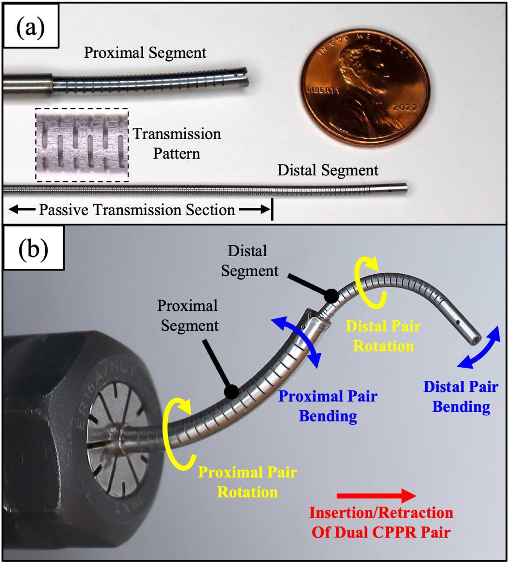
While a single bending segment of tip-attached tubes possesses 3 actuatable DOF, and a triplet of tubes can achieve 4 DOF, we anticipate combining multiple of these bending sections in series to enable higher-DOF robotic devices. This is demonstrated in the video attachment associated with the paper, a still image of which is shown in Figure 2 (b).

To enable independent actuation of the two bending segments, the patterns of the distal tube segment are placed at the end of a transmission portion of tube that has a different cut pattern which is symmetric (no offset stiffness center), flexible (low bending rigidity), and axially and torsionally stiff. Thus, when this pair is actuated, only the distal segment bends, as shown in Figure 6. The flexible transmission portion can be simultaneously curved in any shape without affecting the distal segment actuation, and the distal segment actuation does not affect the reaction forces on the transmission portion. In this way, a CPPR segment can be deployed through the working channel of a long, flexible endoscope, or through the inner lumen of another CPPR segment to create a higher-DOF robot, as shown in Figure 2 and the supplemental video.

Fig. 6.

Demonstration of a two-tube CPPR bending segment with a proximal transmission section, intended for use within a multi-segment CPPR system. The distal CPPR segment actuation is identical whether it is actuated in free space (on the left) or when constrained by a curved overtube (on the right), and the actuation does not exert significant forces on the overtube.

Toward modeling multi-segment robots like this, if the transmission portion of the distal segment is assumed to be axially and torsionally rigid, then each segment’s kinematics can be calculated in series. First, the proximal segment segment kinematics are calculated as described above, with the addition of the bending energy of the transmission portion (which is bent according to the backbone curvature) to the total elastic energy. Then, the distal segment kinematics are calculated independently and transformed by the centerline frame at the end of the proximal segment to obtain the final end effector pose. This approach appears useful because the transmission sections are designed with high axial and torsional rigidity compared to their bending rigidities. Future work may include combined modeling of torsional and axial deformation in the transmission lines.

III. Tube Pattern Design and Parameter Characterization

In this section we discuss the design of the laser cut tubes with offset stiffness centers and characterization of their elastic parameters. For our parameter characterization, we use static finite element analysis (FEA) simulations to calculate the rigidity parameters used in the stiffness matrix ${\mathbf{\text{K}}}_i$ of equation (17) and the stiffness center locations $x_i$ of the patterned tubes.

A. Tube Pattern Designs

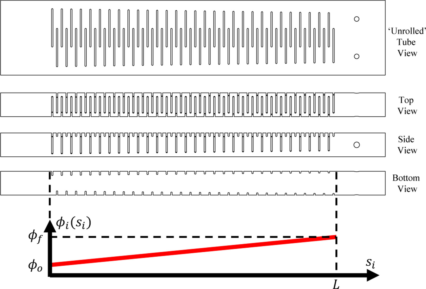
We use a pattern of narrow slots cut into the tube walls with a fiber laser to shift the stiffness center away from the center of the tube cross-section and alter the flexural and torsional rigidity of the tube. The slot pattern contains interleaved slots such that a winding path of solid material remains, similar to so-called “serpentine” beams in MEMs literature [36]. The slotted pattern can vary along the length in order to change the mechanical properties. Three slot patterns, one designed for two-tube CPPRs with constant ${\mathbf{\text{r}}}_i$ (Figure 7), one designed for two-tube CPPRs with varying ${\mathbf{\text{r}}}_i$ (Figure 8) and another designed for 3D three-tube CPPRs with constant ${\mathbf{\text{r}}}_i$ (Figure 9) were used for our validation experiments. In Figures 7(a) and 9(a), the dark regions in the cross-section views represent solid, uncut material.

Fig. 7.

Slotted-tube pattern used for two-tube CPPR validation experiments. Slot parameters are designed using an ’unrolled’ pattern segment that is wrapped over the tube (a). This pattern generates an effective stiffness center along the patterned tube segment and leaves an uncut material ’backbone’ region with intermittently cut material along the segment length. Linearly patterning the segment design down the length of an unrolled tube generates the slotted pattern length $L_i$ (b). The resultant patterned tube is shown from top, side, and bottom views (c).

Fig. 8.

Converging tube design used for the Case 2 CPPR in which the backbone angle ${\varphi }_i$ of each tube linearly tapers down the length of each tube as a function of $s_i$.

Fig. 9.

Slotted-tube pattern used for three-tube CPPR validation experiments. Slot parameters for a unit cell are shown in (a) with the ‘unrolled’ pattern design that is wrapped onto a nitinol tube (b). The patterned tube is shown from a top, side, and bottom views in (c). Note that the additional overlaps from ${\gamma }_i$ create additional slots on the side of the tube, thus enabling improved design of both flexural rigidity values of the tube.

For the two tube CPPRs, we use a linear pattern of overlapping slots, forming a single serpentine pattern along the length of the tube as shown in Figure 7. The slot dimensions include the slot overlap angle ${\psi }_i$, backbone angle ${\varphi }_i$, slot pitch $h_i$, kerf $\lambda$ and the length of tube that contains the slotted pattern $L_i$. In general, increasing the slot overlap angle ${\psi }_i$, decreasing the backbone angle ${\varphi }_i$, and decreasing the slot pitch $h_i$ decreases the flexural and torsional rigidity of the patterned tube. The backbone angle ${\varphi }_i$ is the primary variable that affects the stiffness center offset; the smaller the backbone angle, the greater the stiffness center offset is from the center. The kerf $\lambda$ dictates the amount of tube angulation before the slots close together, such that a larger kerf enables a larger max angulation.

When compared with the larger, rectangular slots used in previous CPPR designs [1], the smaller slot serpentine pattern enables a more homogeneous material response that reduces stress concentrations and prevents mechanical interference of slot edges. While uniform various patterns have been investigated for optimal flexural and torsional properties [37], [38], the serpentine pattern enables us to parametrically and smoothly vary mechanical properties (like stiffness center) down the length of the tube. Furthermore, less material is removed overall, which increases robustness, and the slots can be designed to close at a specific curvature to protect the material (see Section III-D). Finally, the interleaved nature of the slots generally helps to preserve torsional stiffness to a greater degree than patterns with identical slits down the length.

For the tube pattern used in our three tube robot, we used additional overlapping sections in the unit cell pattern that generate serpentine sections on three sides of the tubes. As each tube is required to bend in more than one plane in a three-tube CPPR, having large stiffness asymmetries can make actuation difficult, thus a tube pattern that can achieve near symmetric flexural rigidity values for each tube (i.e. ${\text{(}EI\text{)}}_{x,i}\underset{\_}{\approx }{\text{(}EI\text{)}}_{y,i}$ alleviates this issue. For all tube designs, a pulsed fiber laser was used to machine the slot patterns onto the tubes. The tubes in each prototypes were glued together to their tips using an industrial adhesive (Loctite 430). Laser welding can also provide a strong weld for bonding the tubes together at their distal tips.

B. Young’s modulus calibration

In order to provide accurate FEA results for parameter characterization, we calibrated the Young’s modulus of each tube. The Young’s modulus is found by fitting small deflection force-displacement data from a three-point flexural setup, as shown in Figure 10 and using the Euler-Bernoulli beam equation for a simply supported beam with a midpoint load applied:

$$\delta =\left(\frac{1}{E_i}\right)\frac{F_E{L}_E^3}{48I}$$ (34)

where $E_i$ is the Young’s modulus of the $i^{th}$ tube, $F_E$ is the applied midpoint force, $L_E$ is the length of the simply supported beam, $I$ is the second moment of area of the tube, and $\delta$ is the midpoint displacement of the beam. For our validation experiments, we use three different tube sizes, which are tabulated in Table II. The length $L_E$ used for all tube cases was 90mm. Each tube is simply supported with rollers at each end. A linear actuator (Thorlabs MTS50-Z8), controlled by a DC servo motor controller (Thorlabs KDC101), is used to apply a displacement $\delta$ at the midpoint along the beam. The midpoint force $F_E$ at each displacement is recorded with a force gauge (ATI Mini40) at each applied displacement. A displacement range from 0 to 2mm in 0.1mm increments was used for the modulus calibration. A linear fit is performed on the dictated midpoint displacements as the dependent variable and $F_E{L}_e^3\text{/}48I$ as the independent variable. The slope of the linear fit corresponds to $\text{(}1\text{/}{E}_i\text{)}$. The calibrated Young’s moduli for each tube is tabulated in Table II, which are within the expected Young’s modulus range for nitinol. The coefficient of determination for each fit of (34) was 0.99, ensuring displacements to the tubes were within the linear elastic region of deflection. The experimentally determined Young’s moduli are then implemented into the FEA material model for each tube.

Fig. 10.

Three point flexural test setup used to calibarate the Young’s modulus $E$ of each nitinol tube. The moduli values are then used in our FEA simulations to determine the flexural and torsional properties of our patterned tubes.

TABLE II.

Nitinol Tube Dimensions and Calibrated Mechanical Properties

	$r_o$(mm)	$r_i$ (mm)	$E_i$ (GPa)	$\nu$	$G_i$ (GPa)
Tube 1	1.25	1.18	56.27	0.33	21.15
Tube 2	1.095	1.016	73.43	0.33	27.61
Tube 3	0.900	0.811	68.48	0.33	25.74

C. Parameter Characterization

This subsection details our procedure for calculating the flexural and torsional rigidity values used in (17) and the stiffness center offset ${\mathbf{\text{r}}}_i$ for each patterned tube using FEA. Solidworks Simulation Premium was used as our FEA package, using a linear elastic material model and shell elements. A curvature-based mesh with a maximum element size of 0.1mm and a minimum element size of 0.005mm was used for each simulation. The proximal base of the tube is rigidly fixed in translation and rotation while tip moments are applied at the tip, as shown in Figure 11.

Fig. 11.

FEA Setups for calculating the flexural rigidity about $\text{x}\hspace{0.33em}{\text{(}EI\text{)}}_{i,x}$ (a), flexural rigidity about $\text{y}\hspace{0.33em}{\text{(}EI\text{)}}_{i,x}$ (b), and torsional rigidity ${\text{(}GJ\text{)}}_i\text{)}$ (c). The limits of the colorbar in (a) and (b), $Z_{max}$ and $Z_{min}$, represent the max. and min. displacements in the z-direction and in (c), $u_{max}$ represents the max. resultant displacement in the simulation.

To calculate the effective flexural rigidity values ${\left(EI\right)}_{i,x}$ and ${\left(EI\right)}_{i,y}$ in FEA, we apply moments at the distal tip of the patterned tube of length $L_{FEA}$ and record the resultant bend angle:

$$\begin{gathered} {\left(EI\right)}_{i,x}=\frac{M_x{L}_{FEA}}{{\theta }_x} \\ {\left(EI\right)}_{i,y}=\frac{M_y{L}_{FEA}}{{\theta }_y} \end{gathered}$$ (35)

where $L_{FEA}$ is the length of the patterned tube used in the FEA simulation, $M_x$ and $M_y$ are applied tip moments about the global $\text{x}$- and $\text{y}$-axes respectively, and ${\theta }_x$ and ${\theta }_y$ are the resultant bend angles about the $\text{x}$- and $\text{y}$-axes respectively. Moments at the tip are created by applying two point forces at the tip, each with equal magnitude but opposite directions, separated by a distance of outer diameter of the tube, (i.e. $M_x=2F_x{r}_o$ and $M_y=2F_y{r}_o$). The value of each point force was 0.01N and the bend angle is calculated using a small angle approximation from the maximum and minimum $z$-displacements from the applied moment, ${\theta }_x=\left(Z_{max}-Z_{min}\right)\text{/}\left(2r_o\right)$. We should note that while 3-point bending tests can easily be used to determine the flexural rigiditiy of uniformly patterned tubes, experimental characterization would be much more involved and error prone in the case of variable stiffness (as will be shown in Section IV-C).

To estimate the effective torsional rigidity ${\left(GJ\right)}_i$, we apply a torque $M_z$ about the global z-axis at the tip of the patterned tube and record the resultant rotation ${\theta }_z$:

$${\text{(}GJ\text{)}}_i=\frac{M_z{L}_{FEA}}{{\theta }_z}$$ (36)

To generate the torque $T_z$, we apply four distal forces at the tip to generate a torque about the tube z-axis. Each point force has a magnitude of 0.01N and the proximal base is fixed in translation and rotation. The rotation angle ${\theta }_z$ is similarly calculated using the resulting displacements (i.e. ${\theta }_z=u_{max}\text{/}OD$ where $u_{max}$ is the maximum resultant displacement in the FEA simulation).

To calculate the stiffness center location $x_i$, we use the maximum and minimum z-displacements, $Z_{max}$ and $Z_{min}$ respectively, from the ${\left(EI\right)}_{y,i}$ test:

$$x_i=r_o-\frac{2r_o}{1+\text{|}\frac{Z_{max}}{Z_{min}}\text{|}}$$ (37)

After establishing all the stiffness parameters through the FEA tests, we use these parameters in the kinetostatic model. Figure 12 shows a high level overview of the relationship between the FEA characterization and the kinetostatic model.

Fig. 12.

High-level flowchart the overall modeling paradigm. The dimensions, slot pattern, and material of the tubes are inputs to the FEA-based Parameter Characterization from Section III which outputs the bulk parameters of the slotted pattern. The tube parameters are used in the kinetostatic model derived in Section II. Actuation and external loads are inputs into the kinetostatic, which outputs the resultant shape and pose of the CPPR.

D. Maximum Curvature and Slot Closure

As the bending increases, the curvature will eventually be limited by either material strain or the closure of slots on one of the tubes. Based on the simple geometric assumption that slot contact will happen first at the edges of the overlapped region (spanned by the angle ${\psi }_i$), an approximate analytical relationship between slot design parameters and maximum absolute curvature of a component tube was derived in [39] Equation 4.7, which when solved for curvature gives

$${\kappa }_{i,max}=\frac{\lambda }{h\left|x_i\right|+r_{o}h\hspace{0.17em}\text{cos}\left(\frac{{\psi }_i}{2}\right)-\left|x_i\right|\lambda }$$ (38)

This is a useful heuristic in the design of the slot pattern because we would ideally want to limit the curvature to avoid material strain limits and protect the device, while also ensuring that the slot design will allow the designer’s desired range of curvature. The max curvature according to a material strain limit ${ϵ}_{max}$ can be approximated as:

$${\kappa }_{i,max}=\frac{{ϵ}_{max}}{r_o-\left|x_i\right|}$$ (39)

As long as the slot-closure curvature given by (38) is less than the strain-limit curvature (39), the segment will be somewhat protected from material failure due to accidental overstraining.

IV. Experimental Validation

To validate our kinetostatic model, we compare our model predictions with laser cut nitinol CPPRs for three design cases. Case 1 uses a pair of patterned tubes with constant stiffness center locations along the length of the tube, Case 2 uses a pair of patterned tubes with varying stiffness center and mechanical properties down the length of the tube, and Case 3 uses three tubes with constant stiffness center locations as shown in Figure 9. The rough design goals we had for these prototypes include (1) being able to angulate the device at least 90 degrees for the constant ${\mathbf{\text{r}}}_i$ CPPR design (Case 1), (2) shift the stiffness centers by at least 0.5 mm for a variable tube pattern (Case 2), and (3) maintain reasonably high stiffness. The tube alignment for each design case is shown in Figure 13. For the two tube designs, the backbones are aligned 180° apart from each other about the center of tube pair. For the three tube design, the stiffness centers are 120° apart in the cross-section. For all CPPR prototypes, we weld the distal tips together using an industrial adhesive (Loctite 430). We actuate each CPPR design across its workspace and compare model predictions with the tip positions from the physical robots. For Cases 1 and 2, we also compare model predictions with point loads applied at the distal tip and midpoint along the robot, as well as planar shape experiment comparisons. For our loaded pose experiments, we informally evaluated a range of loads and picked 50g as a representative load that generated significant displacement, but which was well within the payload capacity. During informal tests, we subjected the robot to loads of up to 100g with no adverse effects other than greater displacement at the end-effector.

Fig. 13.

Tube alignments for the two-tube CPPRs (top) and three tube CPPRs (bottom). The principal axes at the center for both alignments indicate the origin of the centerline in relation to the stiffness center locations of each tube.

A. Experimental Setups

We developed two actuation setups for our model validation experiments: a motorized setup for 2-tube CPPRs and a manual setup for the 3-tube CPPR. The 2-tube CPPR setup uses a motorized linear stage (Thorlabs MTS50-Z8) to actuate the inner tube while the outer tube remains fixed. Through-hole drill chucks (Accupro 55162614) are used to grip the inner and outer tubes to the actuation setup. The distal tip positions of the CPPR prototypes are tracked using an electromagnetic (EM) tracker system (NDI Aurora).

For our 3-tube CPPR experiments, we use manual linear stages (Optics Focus MDX-4090-60) to translate tubes 2 and 3 while keeping tube 1 fixed. The drill chucks and electromagnetic tracker system from the 2-tube actuation setup are also used in the 3-tube setup. For each of our experiments, we perform a rigid point-set registration of corresponding experimental and model actuation poses for each case.

B. Case 1: Two-Tube, Constant Stiffness Center Location

Tube 1 serves as the outer tube and Tube 2 is the inner tube from Table II. The slot parameters of the design are shown in Table III and the resultant mechanical properties of both tubes are listed in Table IV. An additional 3mm uncut section is added to the tip of the tube pair to accommodate the EM sensor attachment. We assess the model accuracy by actuating the robot across its planar bending workspace and recording the tip pose at each actuation pose. We compare model predictions with experimental results in (1) free space, (2) distal tip loads applied in the plane of bending, (3) distal tip loads applied out of the plane of bending, and (4) midpoint loads applied in the plane of bending.

TABLE III.

Slot Parameters Used for Case 1 CPPR

	${\varphi }_i$(deg)	${\psi }_i$(deg)	$\lambda$(mm)	$h$(mm)	$L_i$(mm)
Tube 1	90	120	0.15	1.5	30
Tube 2	90	90	0.15	1.5	37.5

TABLE IV.

Mechanical Properties of Case 1 Sheaths

	${\text{(}EI\text{)}}_{i,x}$(Ncm2)	${\text{(}EI\text{)}}_{i,y}$(Ncm2)	${\text{(}GJ\text{)}}_i$(Ncm2)	$x_i\text{(}{s}_i\text{)}$(mm)	${\alpha }_i$(deg)	${\beta }_i$(deg)
Tube 1	17.83	1.25	1.08	−1.09	0	0
Tube 2	20.70	1.85	1.71	0.94	0	0

For the unloaded pose data sets, we actuate the robot across a ±3mm displacement range of the inner tube, actuating the inner tube in 0.25mm increments and recording the distal tip position at each pose. Figure 15(a) shows the range of motion at ±3mm actuation limits and in the straight, unactuated case. We performed a rigid registration of the experimental data to the model data. The largest pose error in the unloaded case occurred at $q=-3mm$, where the error was 1.12mm, approximately 3.6% of the overall active length of the robot. To assess the repeatability of the actuation system, the Case 1 CPPR was actuated up to ±2mm in 0.25mm increments five times. We record the pose error at each actuated configuration, for each registered pose data set. The standard deviation is taken at each actuation pose across the 5 repeated pose data sets. We found that the maximum standard deviation in the error position was 0.04mm, the smallest was 0.007mm, and the mean standard deviation was 0.0207mm. To generate a point force, we attach a 50g weight (∼0.49N) and record the tip position at each pose. The distal tip load applied in-plane case uses an inner tube displacement range of ±1.25mm in 0.25mm increments. The in-plane loading data set is shown in Figure 15(b). The maximum error occurred at the maximum pulling displacement of tube 2, $q_2=1.25mm$, which had a tip error of 0.9mm, approximately 3% of the robot length. The midpoint load applied in the plane of bending used an inner tube displacement range from 0 to 1.5mm and the result is shown in Figure 15(c). The out-of-plane tip loading cases used an inner tube displacement range of ±1mm, recorded poses in 0.25mm increments. The out-of-plane loading data set is shown in Figure 15(d). The tip position error statistics and computation times for the unloaded and loaded cases are recorded in Tables V and VI respectively. As we can see from comparing the results of the in-plane and out-of-plane loading results, the stiffness of the CPPR is much greater in the out-of-plane bending direction. In the straight, cantilevered cases for each loading case $\text{(}{q}_2=0\text{)}$, the transverse deflection while loaded in-plane was 3.72mm and the transverse deflection while loaded out-of-plane was 1.36mm.

Fig. 15.

Case 1 CPPR (constant ${\mathbf{\text{r}}}_i$) actuated while unloaded (a), a tip load applied in the plane of bending (b), a midpoint load applied in the plane of bending (c), and a tip load applied out of the plane of bending (d). A 50g mass was used for the point load cases. The inner tube actuation $q_2$ ranges tested for each case are labeled. Distal tip positions of the CPPR are recorded at each pose and compared with model predictions.

TABLE V.

Tip Position Error Statistics of Case 1

Loading Case	Max. Error (mm)	Min. Error (mm)	Mean Error (mm)	Std. Dev. (mm)
Unloaded	1.12	0.07	0.54	0.24
Tip Load IP	0.90	0.14	0.47	0.29
Mid Load IP	0.44	0.10	0.26	0.14
Tip Load OOP	2.81	0.36	1.24	0.7

TABLE VI.

Case 1 Kinetostatic Model Computation Time Statistics

Loading Case	Max. Time $\text{(}s\text{)}$	Min. Time $\text{(}s\text{)}$	Mean Time $\text{(}s\text{)}$
Unloaded	0.859	0.3594	0.586
Tip Load IP	3.469	2.094	2.537
Mid Load IP	7.469	2.594	4.527
Tip Load OOP	7.266	4.125	5.734

C. Case 2: Two Tube, Varying Stiffness Center Location

In this design case, we analyze the accuracy of the kinetostatic model over a wide range of actuation values, with and without tip loads, on a CPPR with tubes having varying stiffness center locations and mechanical properties along the length of the tube. The tube pattern begins with a stiffness center offset from the center at the base and linearly converges toward the centerline at the distal tip. The rationale behind this design choice stems from the results of [40] and [41] in which a tendon-actuated continuum robot uses converging tendon routing to improve its resistance to tip loads. To create a patterned tube with a varying stiffness center, we use the slotted serpentine pattern shown in Figure 8 and vary the backbone angle ${\varphi }_i$ down the length of each tube. The remaining slot parameters are kept constant down the length of the tube as tabulated in Table VII.

TABLE VII.

Constant slot parameters used for Case 2 CPPR

	${\psi }_i$(deg)	$\lambda$(mm)	$h$(mm)	$L_i$(mm)
Tube 1	90	0.15	1.0	30
Tube 2	90	0.15	1.0	35

We use the following linear function to taper the backbone angle down the length of the tubes:

$${\varphi }_i\left(s_i\right)=\left(\frac{{\varphi }_f-{\varphi }_o}{L_i}\right)s_i+{\varphi }_o$$ (40)

where ${\varphi }_o$ is the backbone angle at $s_i=0$, ${\varphi }_f$ is the backbone angle at $s_i=L_i$. Tubes 1 and 2 use ${\varphi }_o={80}^{\circ }$ and ${\varphi }_f={120}^{\circ }$ in this design case. In addition, the rigidity parameter values will also be affected by the changing backbone design and will need to be functions of $s_i$ as well. To characterize ${\text{(}EI\text{)}}_{i,x}$, ${\text{(}EI\text{)}}_{i,y}$, ${\text{(}GJ\text{)}}_i$, and $x_i$ over the range of backbone overlap angles, we perform a parameter sweep of the constant slotted tube design in Figure 7 using a constant ${\varphi }_i$ using the calibration process used in Section III for Tubes 1 and 2. In these parameter sweeps, ${\varphi }_i$ is the only varied parameter while the remaining slot parameters remained unchanged, as listed in Table VII. The parameter sweep results are plotted in Figure 16 for the flexural and torsional rigidity values and stiffness center locations. A polynomial regression of the parameter sweep data is performed to generate polynomial functions of the rigidity parameters and the stiffness center locations as functions of the backbone angle of the tube. For the rigidity parameters, we use a quadratic polynomial and use a linear fit for the stiffness center locations.

Fig. 16.

Parameter sweep of flexural, rigidity, torsional rigidity, and stiffness center location of tubes 1 and 2 for Case 2 CPPR.

The coefficient of determination of all fits was greater the 0.98, confirming our polynomial order for each case is a good fit for the data. The quadratic fits for the rigidity parameters are implemented into the stiffness matrix ${\mathbf{\text{K}}}_i$ for each tube in equation (17) and the stiffness center linear fits are implemented into ${\mathbf{\text{r}}}_i$ for each tube in equation (1) for the energy minimization in (33).

For the free and in-plane loaded pose data sets of the Case 2 CPPR, we actuated the inner tube ±1.25mm in 0.25mm increments. Like the Case 1 CPPR, we use a 50g weight at the tip. The unloaded pose data set is shown in Figure 17(a) and the loaded pose data set in Figure 17(b). The tip error statistics of the free and loaded data sets are tabulated in Table VIII. The statistics on computation time are shown in Table IX. In free space, the largest error occurred at $q_2=-1.25mm$ and while loaded, the largest error occurred at $q_2=1.25mm$; the second largest error for the loaded pose was $q_2=1.25mm$. In future applications and designs, the mechanical properties could vary down the length either as a means for increasing the strength of the overall structure or for making the tip more flexible to enable tip-first bending.

Fig. 17.

Case 2 (varying ${\mathbf{\text{r}}}_i$) prototype actuated to ±1.25mm in 0.25mm increments in unloaded (a) and tip loaded (b) poses, compared with model predictions.

TABLE VIII.

Tip Position Error Statistics of Case 2

Loading Case	Max. Error (mm)	Min. Error (mm)	Mean Error (mm)	Std. Dev. (mm)
Unloaded	1.05	0.06	0.35	0.26
Loaded	1.21	0.13	0.51	0.36

TABLE IX.

Case 2 Kinetostatic Model Computation Time Statistics

Loading Case	Max. Time $\text{(}s\text{)}$	Min. Time $\text{(}s\text{)}$	Mean Time $\text{(}s\text{)}$
Unloaded	5.125	0.234	3.526
Tip Load IP	5.687	3.531	4.273

D. Computational Speed

While our Matlab implementation of the model prioritizes convenience over speed, we recorded statistics on the computational times required for all experiments on the Case 1 and Case 2 prototypes. These times are recorded in Tables VI and IX. In the case of no-loads, the model could likely be used for real-time control through an optimized C++ implementation. External loading causes an increase in computation likely because the initial guess is farther away from the solution, and the objective function landscape may be more difficult for the solver.

E. Shape Validation Experiments

To assess the model accuracy of predicting the centerline shape of the CPPR, we perform a series of shape validation experiments on the Case 1 and 2 CPPR prototypes in unloaded and tip-loaded configurations. Our experimental setup is shown in Figure 18. We utilize a 24.1 Megapixel DSLR camera (Canon EOS Rebel T8i) and a macro lens (Canon EF 100mm f/2.8L Macro IS USM) for taking images of the prototypes at each pose. For each pose and design case, the camera is placed approximately 2.5m from the CPPR bending plane to mitigate perspective distortion. To convert between pixel coordinates and distances in millimeters, a calibration grid is placed within the bending plane. Shape comparisons of Case 1 and 2 CPPRs in unloaded and tip loaded configurations are compared with the kinetostatic model. Our shape registration process is as follows:

Fig. 18.

Experimental setup used in shape validation experiments. The camera is parallel to the bending plane and is placed approximately 2.5m from the bending plane to mitigate any perspective distortion. A calibration grid (with 5mm line spaces) lies within the bending plane of the CPPR prototypes and is used to convert between the pixel distance in the camera images to millimeter distances in order to compare the prototype shape with the centerline of the model.

1. For each CPPR case and loading scenario, images are captured for each actuated pose.

2. Each actuation pose image is imported into Matlab and using $ginput\text{()}$, the scaling between pixel and millimeter distances is calculated by placing 2 points on the calibration grid in the image.

3. Using $ginput\text{()}$, points are manually placed along the centerline of the CPPR at each slot location for each pose image.

4. A rigid point-to-point registration is performed on the centerline points of the $q_2=0$ image with the corresponding points along the model centerline.

5. The registration transformation is then applied to the other actuation poses. The RMSE is calculated using the experiment and model points along the centerline of the CPPR.

Because the slots have a constant spacing $h$ along the length, for CPPR Cases 1 and 2, corresponding points along the length within the model can easily be extracted for registration and calculated RMSE of each pose. The results of the shape validation are shown in Figure 19 and the RMSE of each case are tabulated in Table X.

Fig. 19.

Shape validation results performed for Cases 1 and 2 in unloaded and tip loaded scenarios. (a) represents Case 1 in free space and actuated to ±3mm, and with a tip load unactuated $\text{(}{q}_2=0\text{)}$ and actuated to $q_2=1mm$ (b). Case 2 in unloaded (c) and tip-loaded configurations (d).

TABLE X.

Shape Validation RMSE

CPPR Case	Loading Case	Actuation Configuration	RMSE (mm)
Case 1	Unloaded	$q_2=0mm$	0.127
		$q_2=3mm$	0.424
		$q_2=-3mm$	0.564
	Tip Load	$q_2=0mm$	0.450
		$q_2=1mm$	0.543
Case 2	Unloaded	$q_2=0mm$	0.466
		$q_2=1mm$	0.469
		$q_2=-1mm$	0.300
	Tip Load	$q_2=0mm$	0.360
		$q_2=1mm$	0.366

F. Case 3: Three Tube, Constant Stiffness Center Location

For our patterned tubes, we use the three serpentine pattern shown in Figure 9 with the design parameters tabulated in Table XII and mechanical properties for each tube are listed in Table XI. The stiffness center locations of each tube are 120° apart from one another about the global z-axis which is inspired by the actuation setups of many tendon-driven [42] and pressure-driven [43] continuum robot designs.

TABLE XII.

Tube Parameters of Case 3 Sheaths

	${\text{(}EI\text{)}}_{i,x}$(Ncm2)	${\text{(}EI\text{)}}_{i,y}$(Ncm2)	${\text{(}GJ\text{)}}_i$(Ncm2)	$x_i\text{(}{s}_i\text{)}$(mm)	${\alpha }_i$(deg)	${\beta }_i$(deg)
Tube 1	1.96	1.78	2.73	−1.12	0	0
Tube 2	1.81	1.78	2.78	−0.983	120	120
Tube 3	1.83	1.89	2.91	−0.764	240	240

TABLE XI.

Slot parameters used for Case 3 CPPR

	${\varphi }_i$(deg)	${\psi }_i$(deg)	${\gamma }_i$(deg)	$\lambda$(mm)	$h$(mm)	$L_i$(mm)
Tube 1	10	70	30	0.15	1.0	30
Tube 2	10	70	40	0.15	1.0	34
Tube 3	10	70	40	0.15	1.0	34

Tube 1 remains fixed for all workspace poses. When either tube 2 or 3 is actuated and the two other tubes remain fixed, the robot bends in the direction of the stiffness center location of the actuated tube. When tubes 2 and 3 are actuated at the same magnitude and direction, the robot undergoes bending in the direction of tube 1. These actuation poses are shown in Figure 20. For our model validation, we actuate tubes 2 and 3 over a ±1mm range in 0.5mm increments. The result comparing the three tube prototype with the model prediction is shown in Figure 21. The tip error statistics are tabulated in Table XIII. The largest tip error occurred for the $q_2=0\text{mm}$, $q_3=1\text{mm}$ configuration and the second largest tip error occurred for the $q_2=1\text{mm}$, $q_3=0\text{mm}$ configuration (which was a 1.21mm error). The largest computation time was 47.74s, the smallest was 0.687s, and the mean was 18.605s. These are much larger times than those seen in the two-tube prototypes, which may be due to larger amounts of stored energy since the tubes in the 3-tube prototype must bend partially about their stiffer axes.

Fig. 20.

Three tube robot actuation poses showing displacements of just tube 2 (left), just tube 3 (middle) and both tubes in equal direction and displacement (right).

Fig. 21.

Workspace of three tube CPPR showing model predictions compared with experimental pose points.

TABLE XIII.

Tip Position Error Statistics of Case 3

	Max. Error (mm)	Min. Error (mm)	Mean Error (mm)	Std. Dev. (mm)
Unloaded	1.98	0.22	0.83	0.44

G. Error Sources

As in the case for CTRs, friction can play a role in model accuracy. As the clearance between the tubes gets smaller and the length of the tubes is larger, it’s more likely to see the effects of friction. In addition to friction, other sources of model error can occur in the parameter characterization process, the CPPR fabrication process, and in unmodeled physical effects such as shear and axial deformations.

Errors in the actual span length $L_E$ used to calibrate the Young’s modulus plays an important role, as the span length term in equation (34) is cubed. Tube mis-alignment, which can occur from the gluing process, can also cause errors. If the clearance between the tubes is too large, the inner tube(s) may be glued to the walls of the outer tube during the glueing process, nullifying the concentricity constraint.

Thermal effects from laser machining have also been found to play a role in altering the microstructure and mechanical properties of Nitinol [44], thus the actual Young’s modulus of the laser patterned tubes may be slightly altered from the uncut tube. In addition, the Kirchhoff tube assumption used in the model does not account for shear and axial deformations. The role of these effects should be further studied in future work as model accuracy would decrease for CPPRs with low axial stiffness and under large axial forces, either from actuation or from external loads. Some of these errors could be mitigated through simultaneous calibration of the rigidity and stiffness offsets of the tubes with the registration of the experimental pose data. Furthermore, these errors can be mitigated, depending on the operation of the CPPR. In robotic applications, errors can be mitigated from the operator in a tele-operated system or through a model-based controller in closed-loop control. However, based on the low errors in the current set of experiments, the influence of these error sources are negligible in the calibration and experimental setups.

V. Discussion and Future Work

We envision that this model will be useful for the design of CPPRs toward future surgical applications, providing kinematic analysis that can account for manipulator interactions with the environment and allow the design optimization of generally patterned tubes for procedure-specific workspaces and force requirements. Furthermore, the model we developed here can be the basis for the development of intrinsic force sensing and control algorithms in future robotic implementations of CPPRs.

There are several areas of future work. In terms of model additions, explicit modeling of transmission shaft compliance, as well as axial and shear deformations in bending segments could be further explored for future CPPR designs. Also, it will be necessary to increase numerical solution speed for use in real-time control and sensing. In design, optimization of tube patterns, both in the bending segments and the flexible transmissions should be further explored, as well as procedure specific designs of surgical manipulators. Multi-segment CPPRs, such as the example shown in Figure 2 and in the video attachment, could be used for robotic surgical applications such as endoscopic submucosal dissection of upper or lower GI cancer. Furthermore, the three-tube CPPR demonstrated from Case 3 also shows potential for robotic actuation since 3D position control can be achieved purely from translations of the tubes, thus enabling an additional “roll” DOF or potentially simplifying actuator design if roll is not desired.

VI. Conclusion

In this paper, we developed a general kinematics model for CPPRs, expanding the capabilities for design and analysis of these tubular robot actuators. The kinetostatic model was derived, starting with the kinematics of a single tube and culminating with the solution of the overall CPPR kinematics using the principal of minimal energy. An FEA-based parameter characterization was demonstrated to estimate the mechanical properties of patterned tubes with offset stiffness centers. Two- and three-tube CPPR design cases were created to test the capabilities of the model. The model shows good agreement for all case designs and has similar levels of accuracy to the state of the art models for other types of continuum robots.

Fig. 14.

Actuation setups for 2-tube CPPRs (top) and 3-tube CPPRs (bottom).

Biographies

Jake A. Childs (Member, IEEE) received the B.S., M.S., and Ph.D. degrees in mechanical engineering from the University of Tennessee, Knoxville, TN, USA, in 2017, 2020, and 2022, respectively. He is currently a mechanical engineer at EndoTheia, Inc., Nashville, TN, USA, a medical device startup commercializing concentric push-pull robots for flexible endoscopy. His research interests include design, modeling, and control of soft/continuum robots and medical devices.

D. Caleb Rucker (Member, IEEE) received the B.S. degree in engineering mechanics and mathematics from Lipscomb University, Nashville, TN, USA, in 2006, and the Ph.D. degree in mechanical engineering from Vanderbilt University, Nashville TN, USA in 2010.

From 2011 to 2013, he was a Postdoctoral Fellow in biomedical engineering with Vanderbilt University. He is currently an Associate Professor in mechanical engineering with the University of Tennessee, Knoxville, TN, USA, since 2013, where he directs the Robotics, Engineering, Applied continuum mechanics, and Healthcare Laboratory (REACH Lab). His research interests include mechanical design, modeling, sensing, and control of medical robots and soft/continuum robots.

Dr. Rucker was a recipient of the NSF CAREER award in 2017.

Appendix

Nomenclature

${\text{(}}^{·}\text{)}$	Derivative with respect to $s_1$
$\text{(}\prime \text{)}$	Derivative with respect to $s$
${\text{(}}^{\wedge }\text{)}$	Mapping that converts ${ℝ}^3$ to $\mathfrak{s}\mathfrak{o}\text{(}3\text{)}$
$\vee$	Inverse of the ${\text{(}}^{\wedge }\text{)}$ operation, ${\text{(}\widehat{\mathit{\text{u}}}\text{)}}^{\vee }=\mathit{\text{u}}$
$s$	Arc length along common centerline
$s_i$	Arc length along undeformed length of $i^{th}$ tube
$n$	Number of tubes in CPPR
$N$	Highest polynomial order in parameterization
${\mathbf{p}}_i$	Global position of stiffness center of the $i^{th}$ tube
${\mathbf{\text{R}}}_i$	Orientation of tube material section plane of $i^{th}$ tube
${\mathbf{\text{r}}}_i$	Stiffness center in cross-section in body-frame
$x_i$	Local $x$-coordinate of stiffness center location
${\mathbf{u}}_i$	Angular rate of change of ${\mathit{\text{R}}}_i$ with respect to $s_i$
$\mathbf{p}$	Centerline position in global coordinates
$\mathbf{\text{R}}$	Orientation of Bishop frame attached to centerline
$\mathbf{\text{t}}$	Tangent vector of centerline position $\mathit{\text{p}}$
$\mathbf{u}$	Angular rate of change of $\mathit{\text{R}}$
$k$	Index of polynomial for parameterized curvatures
$a_k$	Coefficients for x-component of parameterized $u$
$b_k$	Coefficients for y-component of parameterized $u$
$c_{i,k}$	Coefficients of $i^{th}$ tube parameterized curvature
$\mathbf{\text{a}}$	Vector of polynomial coefficients of $a_k$
$\mathbf{\text{b}}$	Vector of polynomial coefficients of $b_k$
${\mathbf{\text{c}}}_i$	Vector of polynomial coefficients of $c_{i,k}$
$\mathbf{\text{x}}$	Coefficients vector of parameterized curvatures
$L$	Length of outermost tube (tube 1)
$q_i$	Actuated linear displacement of $i^{th}$ tube
$\mathbf{\text{y}}$	Vector of state variables
$E_e$	Elastic energy of Kirchhoff tube
$E_F$	Energy from applied point force
$\mathbf{\text{F}}$	Applied point load in global coordinates
$E_f$	Energy from distributed force
$\mathbf{\text{f}}$	Distributed force applied to tube 1
$E$	Total potential energy of CPPR
${\alpha }_i$	Initial angular offset of $i^{th}$ tube at base in CPPR
${\beta }_i$	Distal angular offset of $i^{th}$ tube at tip in CPPR
$\mathbf{\text{g}}$	Nonlinear constraint function
${\text{(}EI\text{)}}_{i,x}$	Flexural rigidity of $i^{th}$ tube about tube x-axis
${\text{(}EI\text{)}}_{i,y}$	Flexural rigidity of $i^{th}$ tube about tube y-axis
${\text{(}GJ\text{)}}_i$	Torsional rigidity of $i^{th}$ tube
${\mathbf{\text{K}}}_i$	Stiffness matrix of $i^{th}$ tube

References

- [1].Oliver-Butler K, Childs JA, Daniel A, and Rucker DC, “Concentric Push–Pull Robots: Planar Modeling and Design,” IEEE Transactions on Robotics, pp. 1–15, September 2021.
- [2].Oliver-Butler K, Epps ZH, and Rucker DC, “Concentric agonist-antagonist robots for minimally invasive surgeries,” in Medical Imaging 2017: Image-Guided Procedures, Robotic Interventions, and Modeling, Webster RJ and Fei B, Eds., vol. 10135. SPIE, March 2017, p. 1013511. [Google Scholar]
- [3].Rox M, Riojas K, Emerson M, Oliver-Butler K, Rucker C, and Iii RJW, “Luminal Robots Small Enough to Fit Through Endoscope Ports: Initial Tumor Resection Experiments in the Airways,” in Hamlyn Symposium on Medical Robotics, 2018.
- [4].Kim J, Choi WY, Kang S, Kim C, and Cho KJ, “Continuously Variable Stiffness Mechanism Using Nonuniform Patterns on Coaxial Tubes for Continuum Microsurgical Robot,” IEEE Transactions on Robotics, vol. 35, no. 6, pp. 1475–1487, December 2019. [Google Scholar]
- [5].Rucker C, Childs J, Molaei P, and Gilbert HB, “Transverse Anisotropy Stabilizes Concentric Tube Robots,” IEEE Robotics and Automation Letters, vol. 7, no. 2, pp. 2407–2414, April 2022. [Google Scholar]
- [6].Lee D-Y, Kim J, Kim J-S, Baek C, Noh G, Kim D-N, Kim K, Kang S, and Cho K-J, “Anisotropic Patterning to Reduce Instability of Concentric-Tube Robots,” IEEE Transactions on Robotics, vol. 31, no. 6, pp. 1311–1323, December 2015. [Google Scholar]
- [7].Azimian H, Francis P, Looi T, and Drake J, “Structurally-redesigned concentric-tube manipulators with improved stability,” in 2014 IEEE/RSJ International Conference on Intelligent Robots and Systems IEEE, September 2014, pp. 2030–2035. [Google Scholar]
- [8].Swaney PJ, York PA, Gilbert HB, Burgner-Kahrs J, and Webster RJ, “Design, fabrication, and testing of a needle-sized wrist for surgical instruments,” Journal of Medical Devices, Transactions of the ASME, vol. 11, no. 1, pp. 0 145 011–145 019, March 2017. [DOI] [PMC free article] [PubMed] [Google Scholar]
- [9].York PA, Swaney PJ, Gilbert HB, and Webster RJ, “A wrist for needle-sized surgical robots,” in Proceedings - IEEE International Conference on Robotics and Automation, vol. 2015-June, no. June. Institute of Electrical and Electronics Engineers Inc., June 2015, pp. 1776–1781. [DOI] [PMC free article] [PubMed] [Google Scholar]
- [10].Eastwood KW, Azimian H, Carrillo B, Looi T, Naguib HE, and Drake JM, “Kinetostatic design of asymmetric notch joints for surgical robots,” IEEE International Conference on Intelligent Robots and Systems, vol. 2016-November, pp. 2381–2387, November 2016.
- [11].Burgner-Kahrs J, Rucker DC, and Choset H, “Continuum Robots for Medical Applications: A Survey,” IEEE Transactions on Robotics, vol. 31, no. 6, pp. 1261–1280, December 2015. [Google Scholar]
- [12].Dupont P, Lock J, Itkowitz B, and Butler E, “Design and Control of Concentric-Tube Robots,” IEEE Transactions on Robotics, vol. 26, no. 2, pp. 209–225, April 2010. [DOI] [PMC free article] [PubMed] [Google Scholar]
- [13].Gilbert HB, Hendrick RJ, and Webster RJ III, “Elastic Stability of Concentric Tube Robots: A Stability Measure and Design Test,” IEEE Transactions on Robotics, vol. 32, no. 1, pp. 20–35, February 2016. [DOI] [PMC free article] [PubMed] [Google Scholar]
- [14].Hur JM, Seo DS, Kim K, Lee JK, Lee KJ, Kim YY, and Kim DN, “Harnessing distinct deformation modes of auxetic patterns for stiffness design of tubular structures,” Materials and Design, vol. 198, p. 109376, 1 2021. [Google Scholar]
- [15].Lu Q and He B, “Kinematics and energy minimization approach for continuum robot,” Mechanisms and Machine Science, vol. 36, pp. 817–827, 2016. [Google Scholar]
- [16].Rucker DC and Webster RJ III, “Statics and Dynamics of Continuum Robots With General Tendon Routing and External Loading,” IEEE Transactions on Robotics, vol. 27, no. 6, pp. 1033–1044, December 2011. [Google Scholar]
- [17].Renda F, Giorelli M, Calisti M, Cianchetti M, and Laschi C, “Dynamic Model of a Multibending Soft Robot Arm Driven by Cables,” IEEE Transactions on Robotics, vol. 30, no. 5, pp. 1109–1122, October 2014. [Google Scholar]
- [18].Jones BA, Gray RL, and Turlapati K, “Three dimensional statics for continuum robotics,” in 2009 IEEE/RSJ International Conference on Intelligent Robots and Systems IEEE, October 2009, pp. 2659–2664. [Google Scholar]
- [19].Rucker DC, Webster RJ, Chirikjian GS, and Cowan NJ, “Equilibrium Conformations of Concentric-tube Continuum Robots,” The International Journal of Robotics Research, vol. 29, no. 10, pp. 1263–1280, April 2010. [DOI] [PMC free article] [PubMed] [Google Scholar]
- [20].Till J, Aloi V, and Rucker C, “Real-time dynamics of soft and continuum robots based on Cosserat rod models,” The International Journal of Robotics Research, vol. 38, no. 6, pp. 723–746, May 2019. [Google Scholar]
- [21].Rucker DC, Jones BA, and Webster RJ III, “A Geometrically Exact Model for Externally Loaded Concentric-Tube Continuum Robots,” IEEE Transactions on Robotics, vol. 26, no. 5, pp. 769–780, October 2010. [DOI] [PMC free article] [PubMed] [Google Scholar]
- [22].Dupont P, Lock J, and Butler E, “Torsional kinematic model for concentric tube robots,” in 2009 IEEE International Conference on Robotics and Automation IEEE, May 2009, pp. 3851–3858. [DOI] [PMC free article] [PubMed] [Google Scholar]
- [23].Black CB, Till J, and Rucker DC, “Parallel Continuum Robots: Modeling, Analysis, and Actuation-Based Force Sensing,” IEEE Transactions on Robotics, vol. 34, no. 1, pp. 29–47, February 2018. [Google Scholar]
- [24].Till J, Bryson CE, Chung S, Orekhov A, and Rucker DC, “Efficient computation of multiple coupled Cosserat rod models for real-time simulation and control of parallel continuum manipulators,” in Proceedings - IEEE International Conference on Robotics and Automation, vol. 2015-June, no. June. Institute of Electrical and Electronics Engineers Inc., June 2015, pp. 5067–5074. [Google Scholar]
- [25].de Payrebrune KM and O’Reilly OM, “On the development of rod-based models for pneumatically actuated soft robot arms: A five-parameter constitutive relation,” International Journal of Solids and Structures, vol. 120, pp. 226–235, August 2017. [Google Scholar]
- [26].Trivedi D, Dienno D, and Rahn CD, “Optimal, model-based design of soft robotic manipulators,” Journal of Mechanical Design, Transactions of the ASME, vol. 130, no. 9, pp. 0 914 021–0 914 029, September 2008. [Google Scholar]
- [27].Wang J, Ha J, and Dupont PE, “Steering a multi-armed robotic sheath using eccentric precurved tubes,” in Proceedings - IEEE International Conference on Robotics and Automation, vol. 2019-May. IEEE, May 2019, pp. 9834–9840. [DOI] [PMC free article] [PubMed] [Google Scholar]
- [28].Wang L, Pedrosa FC, and Patel RV, “Eccentric-Tube Robot (ETR) Modeling and Validation,” in Proceedings of the IEEE RAS and EMBS International Conference on Biomedical Robotics and Biomechatronics, vol. 2020-November. IEEE Computer Society, November 2020, pp. 866–871. [Google Scholar]
- [29].Webster R, Romano J, and Cowan N, “Mechanics of Precurved-Tube Continuum Robots,” IEEE Transactions on Robotics, vol. 25, no. 1, pp. 67–78, February 2009. [Google Scholar]
- [30].Till J and Rucker DC, “Elastic stability of cosserat rods and parallel continuum robots,” IEEE Transactions on Robotics, vol. 33, no. 3, pp. 718–733, June 2017. [Google Scholar]
- [31].Lilge S and Burgner-Kahrs J, “Kinetostatic Modeling of Tendon-Driven Parallel Continuum Robots,” IEEE Transactions on Robotics, April 2022.
- [32].Childs JA, “Improving Strength and Stability in Continuum Robots,” Ph.D. dissertation, The University of Tennessee, Knoxville, December 2022. [Google Scholar]
- [33].Murray RM, Li Z, and Shankar Sastry S, A Mathematical Introduction to Robotic Manipulation CRC Press, December 1994. [Google Scholar]
- [34].Bishop RL, “There is More than One Way to Frame a Curve,” The American Mathematical Monthly, vol. 82, no. 3, p. 246, March 1975. [Google Scholar]
- [35].Lynch KM and Park FC, Modern Robotics: Mechanics, Planning, and Control, 1st ed. Cambridge University Press, July 2017, no. 435. [Google Scholar]
- [36].Barillaro G, Molfese A, Nannini A, and Pieri F, “Analysis, simulation and relative performances of two kinds of serpentine springs,” Journal of Micromechanics and Microengineering, vol. 15, no. 4, pp. 736–746, April 2005. [Google Scholar]
- [37].Ai K Luo Xin Jue, Kim J, Looi T, and Drake J, “Design Optimization for the Stability of Concentric Tube Robots,” IEEE Robotics and Automation Letters, vol. 6, no. 4, pp. 8309–8316, October 2021. [Google Scholar]
- [38].Park S, Kim J, Kim C, Cho KJ, and Noh G, “Design Optimization of Asymmetric Patterns for Variable Stiffness of Continuum Tubular Robots,” IEEE Transactions on Industrial Electronics, vol. 69, no. 8, pp. 8190–8200, August 2022. [Google Scholar]
- [39].Anderson P, “Compliance Characterization and Specification for Surgical Continuum Robots via Modeling, Control, and Design,” Ph.D. dissertation, Vanderbilt University, Nashville, January 2021. [Google Scholar]
- [40].Oliver-Butler K, Till J, and Rucker C, “Continuum Robot Stiffness under External Loads and Prescribed Tendon Displacements,” IEEE Transactions on Robotics, vol. 35, no. 2, pp. 403–419, April 2019. [Google Scholar]
- [41].Childs JA and Rucker C, “Leveraging Geometry to Enable High-Strength Continuum Robots,” Frontiers in Robotics and AI, vol. 8, no. 629871, February 2021. [DOI] [PMC free article] [PubMed] [Google Scholar]
- [42].Neppalli S, Csencsits M, Jones B, and Walker I, “A Geometrical Approach to Inverse Kinematics for Continuum Manipulators,” in IEEE International Conference on Intelligent Robots and Systems, 2008, pp. 3565–3570.
- [43].Skorina EH and Onal CD, “Soft Hybrid Wave Spring Actuators,” Advanced Intelligent Systems, vol. 2, no. 1, p. 1900097, January 2020. [Google Scholar]
- [44].Biffi CA and Tuissi A, “Nitinol laser cutting: microstructure and functional properties of femtosecond and continuous wave laser processing,” Smart Materials and Structures, vol. 26, no. 3, p. 035006, February 2017. [Google Scholar]
Associated Data
This section collects any data citations, data availability statements, or supplementary materials included in this article.