The format of the cognitive map depends on the structure of the environment

Abstract

Humans and animals form cognitive maps that allow them to navigate through large-scale environments. Here we address a central unresolved question about these maps: whether they exhibit similar characteristics across all environments, or—alternatively—whether different environments yield different types of maps. To investigate this question, we examined spatial learning in three virtual environments: an open courtyard with patios connected by paths (open maze), a set of rooms connected by corridors (closed maze), and a set of isolated rooms connected only by teleporters (teleport maze). All three environments shared the same underlying topological graph structure. Post-learning tests showed that participants formed representations of the three environments that varied in accuracy, format, and individual variability. The open maze was most accurately remembered, followed by the closed maze, and then the teleport maze. In the open maze, most participants developed representations that reflected the Euclidean structure of the space, whereas in the teleport maze, most participants constructed representations that aligned more closely with a mental model of an interconnected graph. In the closed maze, substantial individual variability emerged, with some participants forming Euclidean representations and others forming graph-like representations. These results indicate that an environment’s features strongly shape the quality and nature of the spatial representations formed within it, determining whether spatial knowledge take a Euclidean or graph-like format. Consequently, experimental findings obtained in any single environment may not generalize to others with different features.

Introduction

How does the mind represent large-scale, navigable spaces? Decades of research focusing on this question have led to intense debate about the underlying nature of spatial knowledge. Classical theories propose the existence of cognitive maps, which represent spatial locations in Euclidean coordinates, just as they are represented in actual physical maps (Gallistel, 1990; O’Keefe & Nadel, 1978). This Euclidean code allows for the computation of direct vectors between locations and the use of novel shortcuts. However, an alternative hypothesis suggests that spatial knowledge takes the form of cognitive graphs, which represent a subset of locations in terms of the connections (routes) between them, without the use of a global coordinate system (Kuipers, 1982; Warren, 2019). This unresolved debate holds significance not only for spatial navigation but also for cognition in other domains. Spatialized structures such as cognitive maps and cognitive graphs have been proposed to underlie many types of knowledge, including--for example---personality traits (which lend themselves to representation in a multidimensional Euclidean space) and social networks (which lend themselves to representation in a graph-like form). Thus, understanding the circumstances under which these spatialized knowledge structures are formed and used is an endeavor of broad importance.

Here we examine a crucial factor that is often ignored when considering the format of spatial knowledge: the structure of the space being represented. This structure varies across environments, with some environments being more open and others more closed, some having more distal landmarks and others fewer, some having easy to follow connections between subspaces and others having connections that are harder to follow. Most studies employ a single type of environment (e.g. open arena or closed-in maze), and different environmental types are rarely compared within the same study. Although the implicit assumption is often made that findings obtained in one environment should generalize to all, this assumption has not been tested, and there are several reasons to believe that people may in fact form different kinds of mental representations in different kinds of environments.

One line of evidence comes from electrophysiological studies in rodents. When animals navigate in open arenas, hippocampal place cells typically fire in consistent locations irrespective of the direction from which these locations are accessed, indicating a direction-invariant place code (Moser et al., 2008; O’Keefe & Dostrovsky, 1971). In contrast, when animals navigate in linear corridors, place cell firing is modulated by the direction of movement, indicating a direction-dependent representation (McNaughton et al., 1983; Mehta et al., 1997; Muller et al., 1994). Another line of evidence comes from behavioral studies in humans. People navigating in large open environments exhibit behaviors and neural patterns that are consistent with the use of Euclidean cognitive maps (Chadwick et al., 2015; Doeller et al., 2010; Jacobs et al., 2013; Maidenbaum et al., 2018; Shine et al., 2019), whereas people navigating in maze-like environments exhibit behaviors and neural patterns that are consistent with the use of non-Euclidean spatial representations (Chrastil & Warren, 2014; Doner et al., 2022; Ericson & Warren, 2020; He & Brown, 2019; Moeser, 1988; Muryy & Glennerster, 2018; Zetzsche et al., 2009). Taken as a whole, these literatures suggest that the structure of the environment may matter: whereas some environments might be more easily encoded using a Euclidean reference frame, others might be more easily encoded using a cognitive graph consisting of place nodes and their connections (Peer et al., 2021).

If people do tend to form different representations in different environments, this tendency might interact in interesting ways with individual differences in navigational ability. Previous work has shown that people differ in their capacity to form spatial representations of large-scale spaces (Ishikawa & Montello, 2006; Weisberg & Newcombe, 2018). For example, one study found that people learning a virtual environment could be separated into three groups: integrators, who could accurately point to locations in separately-learned parts of the environment; non-integrators, who could only point to locations in the same part of the environment but not across parts; and imprecise navigators, who could not point accurately to any location (Weisberg et al., 2014). However, these groupings were obtained in a single environment with specific features – a large open space without direct visibility across all its parts, traversed by bounded routes. It is unclear how these groupings would generalize to other types of environments, such as open spaces with full co-visiblity or closed environments with constrained routes (e.g. a building with rooms connected by corridors). One possibility is that individual differences might manifest differently across environments with different features. Alternatively, these individual groupings might be stable character traits, perhaps shaped by the environment that the participants grew up in (Barhorst-Cates et al., 2021; Coutrot et al., 2022).

We set out to investigate these ideas by examining how large-scale spatial knowledge differs across newly learned environments with different spatial structure. Participants were randomly assigned to learn one of three virtual environments (Figure 1). The three environments were the same in terms of their graph structure: they all contained nine subspaces that were connected in the same way. Crucially, however, the environments differed in terms of the cues available for determining location and heading in Euclidean space. In the first environment (“open maze”), the subspaces were unwalled patios connected by walkways, contained within a courtyard with distal landmarks. In the second environment (“closed maze”), the subspaces were enclosed rooms connected by corridors. In the third environment (“teleport maze”), the subspaces were enclosed rooms that were connected by “teleporters” located at the room centers. The first two environments were intended to mimic real-life settings that may be represented differently by individuals—the open maze resembled a city park, while the closed maze resembled the interior of a building—whereas the third environment was designed to probe an artificial situation in which participants’ knowledge of the global organization of the environment was limited to the connectivity structure between the subspaces. Following learning, participants performed a series of behavioral tests designed to explore the structure of their spatial representations (Figure S1). We hypothesized that the difference between the environments would affect both the quality and the format of the resultant spatial codes. To anticipate, we found that the environmental structure affected participants’ ability to learn the environment, the format of their mental representation (Euclidean space or cognitive graph), and how these representations varied between participants.

Figure 1: Virtual environments and procedure.

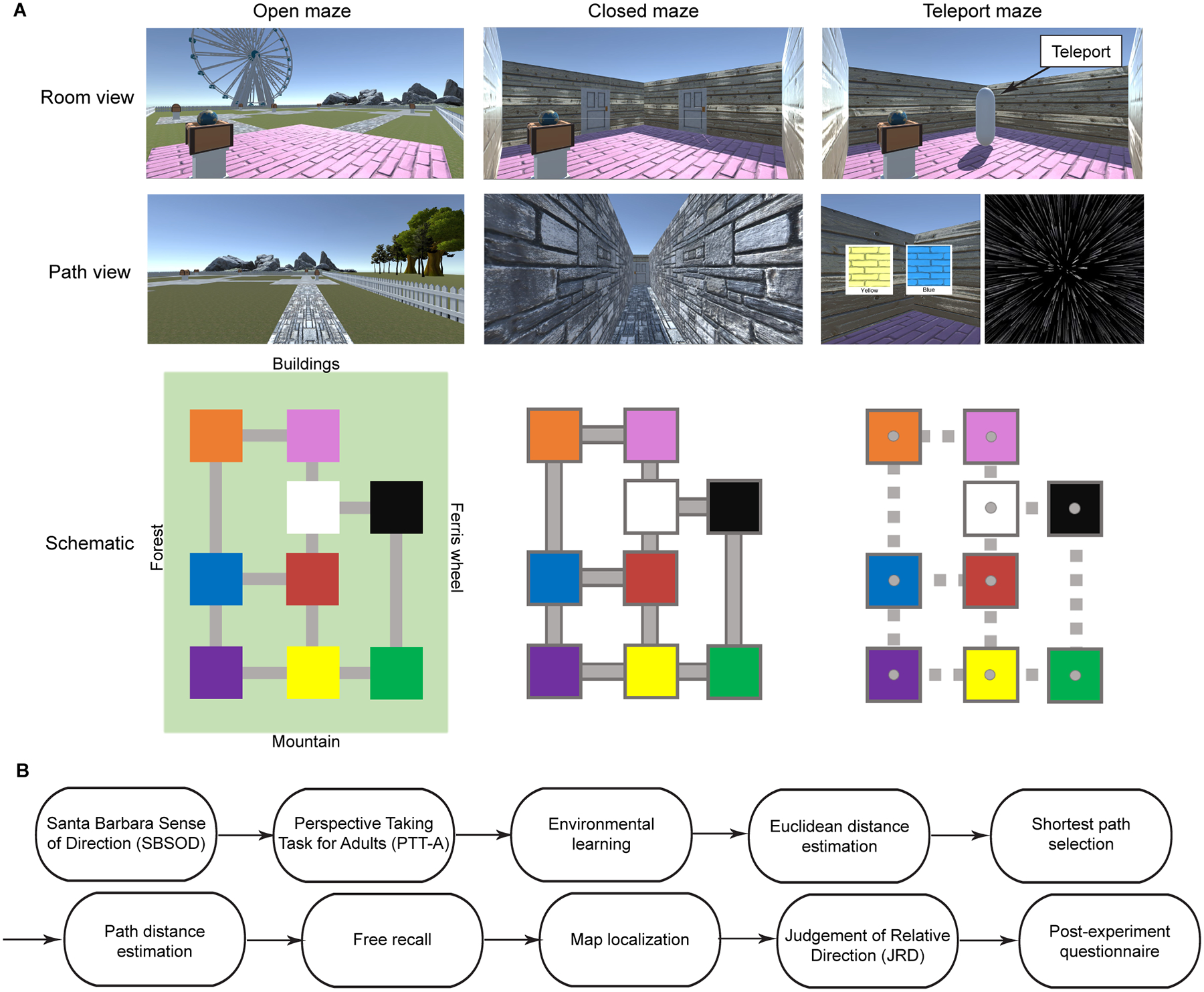
A) All three environments contained nine connected subspaces (patios or rooms), each with a unique floor color and object contained within a treasure chest. In the open-maze condition (left), there were no walls and the entire environment and its surrounding distal landmarks were visible, similarly to a real-life city park. In the closed-maze condition (center), the rooms and connecting pathways were surrounded by walls so that only the immediate surroundings were visible, and participants had to maintain an internal sense of direction and location to navigate, similarly to a real-life building interior. In the teleport maze condition (right), rooms were physically isolated from each other, and participants relied on a system of teleporters to transition between rooms; therefore, they could not maintain a consistent sense of direction and could only learn the connectivity structure of the environment. Each environment is depicted from two viewpoints: Room view, which shows a part of the environment from first person point of view, and Path view, which shows a part of the environment from the pathway, corridor or teleport. Schematic shows that the connectivity structure is the same for all three environments. B) The sequence of the experiment. Participants were administered the Santa Barbara Sense of Direction (SBSOD) and Perspective Taking for Adults (PTT-A) task and were then trained on one of the three environments. Following environmental learning, their spatial knowledge of the environment was tested using a battery of spatial memory tasks. All participants performed all tasks consecutively, except that the Judgment of Relative Direction (JRD) task was omitted for participants in the teleport maze.

Methods

Participants

Sixty healthy individuals were recruited for the study and randomly assigned in equal numbers to three experimental conditions (open maze, closed maze, or teleport maze; 20 participants each). The number of participants was chosen based on power analyses of previous studies that examined spatial localization and pointing accuracy across environments (Barhorst-Cates et al., 2021; Marchette et al., 2017; Mou & Wang, 2015), which indicated that 18–20 participants are needed for effect sizes of 0.67–0.96. Data from 5 participants were excluded before analysis: 3 because they failed to complete the spatial learning task in the allotted time, 1 because they failed to complete the spatial learning task due to nausea, and 1 because their data were lost due a technical error. Five individuals were recruited to replace these participants and assigned to the corresponding conditions. Participants were asked to provide their sex and age: of the 60 participants whose data are reported, 39 identified as female, 21 identified as male, and 1 did not disclose their sex. Mean age was 24 (standard deviation 8.4). Sex and age did not significantly differ between the three groups (proportion female – 0.75, 0.7, 0.53, mean age – 22.3, 26.7, 23.7, for the open, closed and teleport maze respectively; one-way ANOVA, F(57)=1.18,1.47, p=0.32,0.24, for sex and age respectively). All participants provided written informed consent in compliance with procedures approved by the University of Pennsylvania Institutional Review Board. One of the included participants did not have data for the JRD and post-experiment questionnaire due to a technical error, and one did not have data for the PTTA task.

Virtual environments

To test how the structure of a spatial environment affects how the environment is represented, we used Unity 3D software to create three virtual environments (open maze, closed maze and teleport maze). These environments all had the same topological graph structure, but they differed in other features, as described below. Each environment contained nine square (20×20 virtual meter) subspaces (patios or rooms). The subspaces were connected to each other, such that direct travel was possible between each subspace and two or three other subspaces. The nature of these connections differed between environments, as described below, but they always involved the same pairs of subspaces so that the connectivity structure was the same across all three environments (Figure 1A). Each subspace had a unique floor color (black, white, red, pink, yellow, orange, green, blue, or purple), and contained a treasure chest mounted on a pedestal, with an object inside it (ruby, globe, flashlight, book, key, burger, sword, rose, or bottle). Floor colors and objects were randomly assigned to the different rooms for each participant. All objects and environmental elements were purchased from Unity Asset Store.

In the open maze, the subspaces were brick patios without walls. They were laid out on a grassy lawn and were connected by stone pathways (also without walls). Travel was restricted to these pathways. Due to the absence of walls, open visibility was maintained across the entire environment. The lawn was bounded by a low fence that marked off a rectangular area of 130 × 100 virtual meters. Distal landmarks were located beyond the four sides of the rectangle: a rocky mountain range, a storefront, a Ferris wheel and a forest (Figure 1A). The open maze features were selected to mimic real-life open environments, such as city parks, that are open but have visible boundaries and distal landmarks.

In the closed maze, the subspaces were enclosed rooms with bounding walls but no ceiling. They were connected by passageways that also had bounding walls and were open to the sky. There were doors between the rooms and the pathways, so that visibility was always limited to the current room or pathway. There were no distal landmarks (Figure 1B). The closed maze features aimed to resemble real-life closed environments such as building interiors or cities with tall buildings, where visibility between parts of the environment is limited and most of the information available to navigators is the routes between environmental parts.

In the teleport maze, the subspaces were the same rooms as in the closed maze. However, in this case, the rooms had no visible exits. They were connected instead via a system of “teleporters” that were engaged when the participants navigated to an upright 3 virtual meter tall white capsule in the center of each room. Upon reaching the capsule, the names of two or three adjacent rooms, along with corresponding color patches, would appear on the screen. A key press of “1”, “2”, or “3” initiated “teleportation” to the chosen room. During teleportation, a black starry space image appeared on the screen for 2.5 seconds, after which participants landed in a random corner of the target room, facing the center of the room. Thus, teleportation moved participants from one room to another without allowing them to maintain a consistent sense of direction. The connections between rooms through the teleporters were exactly the same inter-room connections as in the open and closed maze environments. As in the closed maze environment, there were no distal landmarks (Figure 1C). The teleport maze did not resemble real-world environments but was instead aimed to study whether people can navigate and form accurate representations based on connectivity structure alone, without the ability to continuously track their global heading or location.

Experimental Procedures

Overview

At the beginning of the experiment, participants completed the Santa Barbara Sense of Direction (SBSOD) scale and the Perspective Taking Task for Adults (PTTA) to test their baseline spatial abilities. Participants assigned to the teleport maze condition then completed a brief slideshow tutorial explaining how the teleporter system operated. All participants then completed the environmental learning task, which was intended to teach them about the spatial arrangement of the environment and the location of the objects within it. The knowledge that they obtained was then assessed by a series of spatial memory tasks: Euclidean distance estimation, shortest path selection, path distance estimation, free recall, map localization, and Judgment of Relative Direction (JRD). Finally, participants filled out a post-experiment questionnaire (see Figure S1).

The experiment was performed in a single behavioral session, which was administered virtually while being monitored by the experimenter through the Zoom video conferencing software. Each participant downloaded the experimental software to their personal computer, on which the experiment was administered while remotely sharing the view of the screen with the experimenter. Experimental data was continuously transmitted to the experimenter during the session. The session lasted between 1.5–2 hours (mean = 79.6 minutes, SD = 23.2 minutes). Below we describe each experimental task in detail. All tasks were programmed using Unity 3D software and were self-paced.

Santa Barbara Sense of Direction (SBSOD)

Participants completed the Santa Barbara Sense of Direction (SBSOD) scale, a 15 question self-assessment of their navigational ability (Hegarty, 2002). On each trial, a phrase related to spatial ability appeared on the screen, and participants asked to rank how much this phrase describes them on a scale of 1 to 7.

Perspective Taking Task for Adults (PTTA)

Participants completed the Perspective Taking Task for Adults (PTTA), which is designed to evaluate the ability to take a spatial perspective other than one’s own (Frick et al., 2014). On each trial, participants viewed an image of a toy person taking a picture of 3 colored geometric shapes, and were instructed to select one out of eight photos that accurately displays the view from the photographer’s perspective. Before the task, participants viewed a brief tutorial slideshow to become familiar with the task. Participants were instructed to complete as many trials as possible within 3 minutes.

Environmental learning task

The environmental learning task was intended to teach participants the structure of the environment and items’ locations in it. During this task, participants freely navigated the virtual environment using the computer keyboard, while viewing it from a first-person, ground-level perspective. The task was divided into six stages. Stages 1–3 focused on learning the room locations; stages 4–6 focused on learning the object locations.

In each stage, participants were required to navigate to 9 navigational goals (rooms or objects) in a random sequence. Each stage began with short instructions, after which the name and image of the first navigational goal (room or object) was shown at the top of the screen. Participants were required to navigate to the goal and press the spacebar key when they arrived at its location (inside the goal room, or next to the treasure chest containing the goal object). If they pressed the button at the correct goal location, the next navigational goal was displayed. If they pressed the button at an incorrect location, an error message was displayed, and they had to continue searching until they reached the correct location, at which point they moved on to the next trial. After all nine rooms or objects were found, participants were cued to search again for any items they made errors on, and they only moved on to the next stage after they found all nine goals in errorless trials. A counter at the top of the screen indicated how many rooms or objects had been found successfully during the current stage. Participants were randomly placed in the center of one of nine rooms at the start of stage 1, and started each subsequent stage from the ending position of the previous stage.

In stages 1–3, participants searched for the rooms denoted by their floor colors. In stage 1, each room’s floor color was made visible as soon as the participant was within the room boundaries. This meant that they could always see the floor color of the room they were in, but could not see the floor colors of distant rooms in the open maze, even though the rooms themselves were visible. In stage 2, each room’s floor color was only visible once the participants indicated that they were at the goal room, forcing participants to use their memory for the floor colors. Stage 3 was similar to stage 2, but all rooms had to be found in errorless sequence in order to finish the task. If an error was made, the stage started over at the beginning, with a new random sequence of trials. Throughout stages 1–3, each treasure chest was opened as soon as participants entered its corresponding room, making the objects visible (even though they were not yet relevant to the task).

In stages 4–6, participants searched for the objects. In stage 4, the treasure chest in each room opened as soon at the participant entered the room, revealing the object within. In stage 5, objects remained hidden inside the treasure chests until participants approached one of the chests and indicated that it was the goal location, at which point the chest opened. Stage 6 was similar to stage 5, but participants were required to find all objects in an errorless sequence, and had to repeat the whole stage from the beginning if they made a mistake. Throughout stages 4–6, floor colors were made visible as soon as participants entered each room.

The learning task was limited to 65 minutes; participants who exceeded this limit were not tested further. The gradual learning, repetition of incorrectly remembered rooms and objects at the end of each stage, and requirement for perfect color/object finding in stages 3 and 6 ensured that participants who completed the learning task accurately encoded all of the room and object locations.

Euclidean distance estimation task

This task tested participants’ knowledge of direct-line (Euclidean) environmental distances. On each trial, the names of two objects were presented, one on the left and one on the right side of the screen. Participants then typed in their estimate of the direct-line (Euclidean) distance between the two objects, in feet. All possible pairs of objects were used, resulting in 36 trials.

Shortest path selection task

This task tested participants’ knowledge of the connectivity structure between rooms. On each trial they saw the name of a starting room (indicated by floor color) and the name of a target object. Below these on the screen, they saw the names and color patches corresponding to the rooms (two or three) that were connected to the starting room, ordered from left to right in a random order. Their instructions were to choose the connecting room that would take them from the starting room to the target object using the shortest possible path. All possible room-object combinations were queried, with the exception of combinations for which target objects were in rooms adjacent to the starting room and combinations for which there was no correct answer because all selections had a similar shortest path distance. With these exclusions, there were 36 trials. Participants were queried on the first step of the route instead of the whole route to keep the experiment within a reasonable length of time.

Path distance estimation task

This task tested participants’ knowledge of the lengths of the routes connecting different parts of the environment. On each trial, they viewed the names of two objects, presented on the left and right side of the screen. They were instructed to type their estimate of the time (in seconds) it would take them to travel between the two objects. All possible pairs of objects were used, resulting in 36 trials.

Free recall task

This task tested whether participants’ recall order was shaped by the rooms’ connectivity or distance (Miller et al., 2013). Participants were asked to type the names of the objects in the maze in any order, pressing the “return” button after each name to move on to the next line. They then pressed the “finish” button when they had recalled as many objects as possible. Entered object names remained visible along with a counter indicating the number of entered objects.

Map localization task

This task measured participants’ explicit knowledge of the locations of each room and object. On each trial, they were presented with the name and picture of an object on the screen, or the name and picture of a floor color corresponding to one of the rooms, along with an empty rectangle proportional to the environment size. They were instructed to click the cursor within the rectangle to indicate the location of the indicated item, at which point a red dot appeared in the clicked location; participants could click again to reselect the location as many times as they wanted before finalizing their answer by clicking a “continue” button. Items remained visible on the screen in their selected location in the following trials, allowing participants to place subsequent items relative to previously selected locations (and not just relative to the overall environmental boundary). Each room and object (18 total) was queried, in random order.

Judgment of Relative Direction (JRD) task

This task tested participants’ knowledge of the directional relationships between parts of the environment. On each trial, they saw the names of two floor colors (corresponding to two rooms) and one object. They were instructed to imagine that they were standing in the first room (starting room), looking toward the second room (facing room). They were then asked to indicate the direction of the object (target object) by rotating an arrow on the screen from 0 to 360 degrees. Each possible starting-facing room combination was queried, for a total of 72 trials. Target objects were never in the starting or facing rooms, and each target object was used an equal number of times. Only participants in the open and closed maze environments completed the JRD task.

Quantification and Statistical Analysis

Santa Barbara Sense of Direction (SBSOD)

Each participant’s self-rated navigational ability was measured by averaging across all SBSOD questions (taking into account questions that are reverse scored). The resulting SBSOD scores did not significantly differ between the open maze, closed maze and teleport maze participant groups (F(57)=0.26, p=0.77, one-way ANOVA). Scores across participants were then correlated to individual performance in each spatial memory task.

Perspective Taking Task for Adults (PTTA)

Each participant’s perspective taking ability was measured by scoring the number of PTTA trials answered correctly within the time limit, out of a maximum of 32. PTTA scores did not significantly differ between the open maze, closed maze and teleport maze participant groups (F(57)=2.66, p=0.08, one-way ANOVA). Scores across participants were then correlated to performance in each spatial memory task.

Environmental learning task

To verify that participants learned the environmental structure and used it to navigate (instead of walking randomly until encountering the target room/object), we calculated a measure of navigational efficiency for each participant in the following manner. First we calculated, for each trial, the length of the path that the participant took from the starting location (i.e. the location of the room/object that was the goal on the previous trial) to the goal location. In the open and closed mazes, the physical path length between the room centers was used (i.e. virtual meters); for the teleport maze condition, the path length was the number of rooms through which the participant passed (since all inter-room transitions were of similar length in this condition), and 1 was subtracted from this number (since the floor color of the target room, or the room containing the target object, was always visible upon reaching the teleporter in the room preceding the target). Then, for each trial, chance level performance was calculated by generating 1000 random walks between the starting and goal location and averaging the path lengths of these random walks. The true path length was then divided by the average chance path length to obtain a path efficiency ratio. These ratios were compared to 1 (the null hypothesis of no difference between chance and actual performance) using a one-sample one-tailed t-test across participants in each condition, with FDR-correction across conditions. Stages 1 and 4 were not included in this calculation because paths in these stages were implemented prior to learning room and object locations.

To test for possible use of cognitive graph knowledge during participants’ route decisions, we examined trials for which there were two pathways of equal length but different number of intervening rooms between the starting and target locations. By examining these trials, we aimed to determine whether participants relied on cognitive graph knowledge (room connectivity structure) rather than solely relying on absolute Euclidean locations and distances. In these trials, a preference for the route with fewer intervening rooms would indicate navigation guided by room connectivity, while an equal chance of selecting each route would suggest reliance solely on Euclidean knowledge. We calculated the proportion of these trials on which participants chose the route with the lower compared to the higher number of intervening rooms. This value was compared to the null hypothesis of no route preference (0.5) using a one-sample two-tailed t-test in each environmental condition, with FDR-correction across conditions. These values were computed for the open and closed maze conditions. They were not calculated in the teleport maze, because path length and number of intervening rooms were identical quantities in this condition.

Euclidean distance estimation task

To assess participants’ knowledge of absolute distance between locations, task accuracy was quantified by calculating the correlation between the estimated distance and the veridical Euclidean distance across trials. The use of correlation provided a scale-invariant measure, mitigating biases from participants who may have consistently overestimated or underestimated distances in feet in the virtual environment. Accuracy was compared to chance for each environment by using a one-sample one-tailed t-test against a zero baseline, FDR-corrected across the three environments. Differences between conditions were tested using a one-way ANOVA with Tukey-Kramer post-hoc tests.

To test if participants’ distance estimations were affected by cognitive graph knowledge (instead of solely corresponding to the true Euclidean distances), for each participant, we calculated the correlation between the estimated distances across trials and the shortest path length between rooms. We compared this value to the correlation between estimated distances and Euclidean distances (i.e. task accuracy) using a paired-samples two-tailed t-test. We reasoned that participants who used graph-knowledge to estimate distances would show greater correlation with path distance than with Euclidean distance. This analysis was not performed for participants in the teleport maze, because these participants only had direct knowledge about the number of intervening rooms, not path length or Euclidean distance.

Shortest path selection task

To measure participants’ knowledge of the connectivity between rooms, we calculated the percentage of correct responses for each participant (i.e. the percentage of trials for which participants correctly chose the shorter path). In the open and closed mazes, correct responses were based on the veridical path length. In the teleport maze, correct responses were based on the number of rooms connecting the starting and target objects (since no path length information was available in this condition). Chance performance was estimated for each maze by making 1000 random answer selections for each question (average chance level accuracy - 0.49 for the open and closed maze conditions, 0.45 for the teleport maze condition). Accuracy was compared to chance using a one-sample one-tailed t-test across participants, with FDR-correction across conditions. Differences between conditions were tested using a one-way ANOVA with Tukey-Kramer post-hoc tests.

To test whether participants incorporated cognitive graph knowledge in their responses, we examined trials in the open and closed mazes for which there were two pathways of equal veridical length but different number of intervening rooms between the starting and target rooms. We calculated the fraction of these trials on which participants chose the route with the lower compared to the higher number of intervening rooms. This value was compared to the null hypothesis of no route preference (0.5) using a one-sample two-tailed t-test, with FDR-correction across mazes. In addition, we conducted a secondary analysis by considering only intervening rooms that served as decision points, disregarding rooms with only one entry and one exit point (since these rooms may have been treated as parts of the route instead of as distinct nodes).

Path distance estimation task

To measure participants’ knowledge of the length of environmental routes, task accuracy was computed for each participant by taking the correlation between the estimated distance on each trial (quantified in terms of travel time) and the veridical shortest path distance between objects (for the open and closed maze conditions’ participants) or the veridical minimal number of rooms connecting the starting and target objects (for the teleport maze condition participants, since inter-room transitions did not differ in length in this condition). Above-chance performance in each environmental condition was measured using a one-sample one-tailed t-test across participants in each condition against a zero baseline, with FDR-correction across conditions. Differences between conditions were tested using a one-way ANOVA with Tukey-Kramer post-hoc tests.

Free recall task

The relation between recall order and objects’ spatial distance was measured by calculating the distance between each pair of consecutively-recalled objects, averaging these values for each participant, and comparing these values to chance-level distances (estimated using 1000 random permutations of object names) using a one-sample one-tailed t-test across participants in each condition, with FDR-correction across conditions. Differences between conditions were tested using a one-way ANOVA with Tukey-Kramer post-hoc tests.

Map localization task

To test participants’ knowledge of the overall environmental configuration, task accuracy was assessed by taking each participant’s localization responses and using a gradient descent algorithm to translate, scale, mirror, and rotate these responses by multiples of 90 degrees until they best fit the true configuration. Accuracy was then determined by measuring the average distance between each object’s marked location and its true location. These values were compared to chance-level performance (estimated using the same process for 1000 random localizations of 9 items), using a one-sample one-tailed t-test across participants in each condition, with FDR-correction across conditions. Differences between conditions were tested using a one-way ANOVA with Tukey-Kramer post-hoc tests.

We also tested whether participants might have represented the environment as a graph with equal distances between rooms. Since there is no 2-dimensional configuration with exact equidistance between rooms, we created an approximate model of an equidistant graph by taking the rooms’ connectivity structure and utilizing a spring-embedding algorithm using Cytoscape 3.9.1 ((Kamada & Kawai, 1989; Shannon et al., 2003); Figure 3E). Subsequently, we assessed localization accuracy relative to this structure using the same methodology described above (involving rotating, translating, mirroring, and scaling the data to the configuration that best matched the model, followed by measuring the average distance between the marked locations and the corresponding locations in the model).

Judgment of Relative Direction (JRD) task

To test participants’ knowledge of the directions between environmental elements, task accuracy was computed as the mean angular distance between participants’ responses and the veridical object directions. These values were compared to chance-level performance (90 degrees average deviation) using a one-sample one-tailed t-test across participants in each condition, with FDR-correction across conditions. The difference between the open and closed maze conditions was tested using a two-sample two-tailed t-test.

Individual variability analysis

To investigate individual variability in environmental learning, we used the map localization task results to assign participants to groups, because this task provides the most direct test of participants’ knowledge of environmental layout. Employing K-means clustering (K=2) on the performance data from the map localization task, we divided the 60 participants into two groups (participants with good and bad knowledge of the veridical environmental structure). To confirm the distinctiveness of these groups, we computed the silhouette value of the clustering and compared it to the silhouette values obtained from 1000 iterations of randomly-generated data (in the same value range) divided into two groups using k-means clustering. The silhouette value of the original grouping exceeded that of 99% of the random groupings, demonstrating significant separation between the groups (p=0.01). Further validating this grouping, dividing the data to two clusters based on the median value yielded nearly identical results, with only two participants differing in their classification. The resulting groups of participants were subsequently named “integrators” (32 participants) and “non-Integrators” (28 participants), following Weisberg & Newcombe 2018. Within the integrators group, 18 participants were in the open maze, 9 participants were in the closed maze, and 5 participants in the teleport maze. Within the non-Integrators group, 2 participants were in the open maze, 11 participants were in the closed maze, and 15 participants were in the teleport maze. To assess the difference in distribution of integrators and non-integrators between the groups, we used a Chi-square test.

To investigate the effect of individual variability on task performance, we analyzed the accuracy of integrators and non-integrators in the Euclidean distance estimation task, shortest path selection task, path distance estimation task, and JRD, in each environment separately. Since there were few non-integrators in the open maze or integrators in the teleport maze, these two groups (open maze non-integrators and teleport maze integrators) were omitted from the analyses. Differences between the remaining four participant groups (open maze integrators, closed maze integrators, closed maze non-integrators and teleport maze non-integrators) were tested for each task using a one-way ANOVA with Tukey-Kramer post-hoc tests. The resulting p-values were FDR-corrected across tasks.

Bayesian analyses and post-hoc power analyses

To further validate our statistical analyses, we complemented the traditional hypothesis testing with Bayes factor (BF10) calculations for all statistical comparisons. Bayesian analyses were conducted using the BayesFactor toolbox (Krekelberg, 2022). Effect strengths were interpreted following standard guidelines (BF10>10 – strong evidence, 10>BF10>3 – moderate evidence; (Van Doorn et al., 2021)).

Additionally, we assessed the replicability of the observed effects by conducting post-hoc power analyses of each of the paper’s significant effects using G*Power 3.1 (Faul et al., 2009). The power analysis indicated that the majority of the study’s effects should be detected with sufficient power (β=80%) with sample sizes ranging from 4 to 18 participants per condition. Detailed information on Bayesian statistics, effect sizes, power analysis results, and other statistical values is provided in Table S1.

Transparency and Openness

We report how we determined our sample size, data exclusions (if any), manipulations, and measures in the study. This study was not preregistered. All data and analysis codes are publicly available at: https://osf.io/adcfk/.

Results

The structure of the environment affects the accuracy of spatial knowledge

Each participant was familiarized with one of the three virtual environments through a multi-stage training procedure. Participants first learned to navigate between the rooms (defined by their floor colors), and then learned to navigate to objects located in “treasure chests” within each room. By the end of the training, participants were able to use their memory to navigate to all rooms and objects without error, even in the absence of any floor colors or visible objects. Their routes to the targets were significantly shorter than a random walk (p<0.01 for all three environments; see Table S1 for full statistical results of all analyses), indicating that they encoded representations of the spatial organization of the environment and used these representations to guide their movements.

Participants then performed a series of memory tasks to assess their spatial knowledge of the learned environment in detail. Three tasks were designed to test Euclidean knowledge (Euclidean distance estimation, map localization, and judgment of relative direction) and two were designed to test graph-based knowledge (path distance estimation, shortest path selection). All tasks were administered to all participants, with the exception the judgment of relative direction task (JRD), which was not administered to participants in the teleporter maze because directions between rooms are not defined in this environment.

In all three environments, performance in all tasks was better than chance (all ps<0.01; Figure 2A–E, Table S1). However, we also observed consistent differences in performance between the environments: accuracy was highest in the open maze condition, intermediate in the closed maze condition, and lowest in the teleport maze condition. These differences between environments were confirmed by ANOVA for the Euclidean distance estimation, map localization, path distance estimation, and shortest path selection tasks (all Fs>18, all ps<0.0001; FDR-corrected across tasks) and by t-test for the JRD task (t(1,37)=2.3, p=0.025). Tukey-Kramer post-hoc tests found significant differences between the open and closed maze for the Euclidean distance estimation, map localization, path distance estimation, and shortest path selection tasks (all ps<0.05) and significant differences between the closed and teleport maze for the Euclidean distance estimation and shortest path selection tasks (p=0.0497, 0.006, respectively). Post-hoc tests of the closed vs. teleport maze difference fell short of significance for the map localization and path distance estimation tasks (p=0.11, 0.074, respectively). Bayesian analyses provided strong evidence (Bayes Factor>10) for pairwise differences between the open and closed maze in all tasks except JRD, where there was only weak evidence (BF10=2.5), and there was moderate or weak evidence for pairwise difference between the closed and teleport maze across the tasks (BF10 values=1.07–4.93). Notably, the same pattern of performance across environments was observed for the three tasks that assessed Euclidean knowledge (Euclidean distance estimation, map localization, JRD) and the two tasks that assessed graph-based knowledge (path distance estimation, shortest path selection).

Figure 2: Accuracy of spatial memory differs across environments.

A-E) Performance in spatial memory tasks. In all environments and tasks, participants performed above chance level (dashed line), indicating that they acquired information on the environment’s spatial layout. However, spatial memory accuracy differed across tasks: it was highest in the open maze condition, lower in the closed maze condition, and lowest in the teleport maze condition, indicating that the gradual removal of location and direction cues impaired spatial memory despite the similar layout and connectivity of all environments. F) Free recall of object names: objects’ recall order was related to inter-object spatial distances in the open and closed maze conditions, but not in the teleport maze condition. Grey dots represent individual participants’ data; colored dots indicate group means (green – open maze, red – closed maze, blue – teleport maze); error bars indicate standard error of the mean; asterisks represent significant above-chance performance; full lines represent significant differences between adjoining conditions.

We also administered a free recall task on the object names. Previous work has shown that the order of free recall can be shaped by the spatial proximity of objects, such that closer items are more likely to be recalled in sequence (Hirtle & Jonides, 1985; Miller et al., 2013; Peer & Epstein, 2021). Consistent with this prior work, the order of object recall was related to the both the Euclidean and path distance between objects in the open maze (Euclidean p=0.003; path p=0.005) and in the closed maze (Euclidean p=0.02; path p=0.02; all ps FDR-corrected across environments). Bayesian evidence for these relationships was strong in the open maze (BF10=67, 49, respectively; Table S1) and moderate in the closed maze (BF10=7.41, 8.15, respectively). In the teleport maze, recall order was not related to either Euclidean or path distance (p=0.56, 0.12, respectively).

Taken together, these results demonstrate that participants can acquire information about the spatial structure of different environments, even in environments like the teleport maze where spatial structure is defined by connectivity relationships alone. However, there is an ordering of spatial memory accuracy that relates to the richness of the location and direction cues. Accuracy is highest in the open maze, where participants can determine their location and heading directly through perception. Accuracy is intermediate in the closed maze, where participants can use perception to determine their local (within-room) location and heading, but can only determine their global (across-rooms) location and heading by keeping track of these quantities as they move from room to room. Accuracy is lowest in the teleport maze, where any inference about global location and heading must be made indirectly because there were no cues indicating these quantities as the participants teleported from room to room. Thus, the structure of the environment affects the quality of the spatial representations formed.

The structure of the environment affects the format of spatial knowledge

We next investigated whether the structure of the environment affects not just the accuracy of learned spatial representations, but also their format. We were specifically interested in the distinction between map-like and graph-like representations. Some researchers have argued that spatial knowledge typically takes the form of a map-like Euclidean code (Gallistel, 1990; O’Keefe & Nadel, 1978; Siegel & White, 1975), while others have argued that it typically takes the form of a graph consisting of nodes and edges (Kuipers, 1982; Warren, 2019). We previously suggested that Euclidean representations might be more common in open environments, whereas graph-like representation might be more common in closed environments (Peer et al., 2021). Here we tested this idea in four analyses.

First, we examined route preferences during the learning task, focusing on trials in the open and closed mazes that had two possible routes toward the target, each with the same Euclidean path length but a different number of intervening rooms (Figure 3A). We reasoned that if participants relied on a purely Euclidean cognitive map, then Euclidean distance to goal should be the only consideration for route choice, and both routes should be selected with equal probability. If, however, participants relied on a graph-like representation, then they should prefer to take the path with fewer intervening rooms, because this involves travelling over fewer graph edges. Moreover, if graph-like representations are more common in closed environments, this bias would be stronger in the closed maze than in the open maze. Consistent with these predictions, participants in the closed maze preferred routes passing through a smaller number of rooms (p=0.001), while participants in the open-maze participants did not (p=0.17, FDR-corrected across environments), and the difference in route preference between the mazes was significant (t(38)=2.11, p=0.04). Thus, these results found evidence for preferential use of graph-like representations in closed environments, though we must caveat this by noting that Bayesian evidence for the open vs. closed maze difference was weak (BF10=1.7, Figure 3B, Table S1).

Second, we tested for analogous effects in the shortest-path selection task. Once again, we focused on trials in which participants were asked to choose between two paths that had equal Euclidean length but different numbers of path segments. We found that closed-maze participants consistently selected routes with fewer intervening rooms, indicating the use of a graph-like representation (p=0.004, FDR-corrected across mazes). Open maze participants exhibited a similar but weaker tendency, which did not reach significance (p=0.07; Table S1). There was no significant difference in the inclination to use graph knowledge between the two environments (p=0.22; Figure 3C, Table S1). Similar results were observed when path lengths were defined by number of intervening decision points (i.e. rooms with two possible exits) rather than number of intervening rooms (p=0.0002, 0.068, for the closed and open maze respectively; Table S1). Thus, these results provide evidence for the use of graph-like representations, but do not provide evidence for preferential use of graph-like representations in closed environments.

Third, we examined distance estimates in the Euclidean distance estimation task. We reasoned that if participants utilized a graph-like code instead of (or in addition to) a map-like code, then their Euclidean distance estimates should be affected by the path distance between the two items on each trial, even though path distance is not what the task queries. To test this idea, we correlated participants’ estimated distances on each trial to both the veridical Euclidean distances and the veridical path distances. In the open maze, participants’ Euclidean distance estimates were equally correlated with both Euclidean and path distance (mean r=0.72,0.74, respectively, p=0.38 for the difference; Figure 3D, Table S1). In the closed maze, however, their Euclidean distance estimates were more highly correlated with path distance than Euclidean distance, suggesting the use of graph knowledge (r=0.46,0.42, respectively, p=0.009 for the difference). However, this higher correlation for path vs. Euclidean was not significantly greater in the closed maze compared to the open maze (p=0.09). Thus, this analysis found evidence for the use of graph-like representations in the closed environment, but did not find evidence for preferential use of graph codes in this environment.

Finally, we examined participants’ responses in the map localization task. To test for preferential use of map-like vs. graph-like codes, we analyzed the data with reference to two ground truth models: 1) the actual Euclidean structure of the space and 2) a graph-like structure in which rooms are assumed to be approximately equidistant from each other (see Methods). The object and room locations reported by the open maze participants were more consistent with Euclidean structure than with equidistant graph structure (p=0.00005, FDR corrected across environments; Fig. 3E, Table S1), whereas responses in the closed maze and teleport maze were better fit by the equidistant graph model (p=0.04, 0.00004). Bayesian evidence supporting these preferences was strong in the open and teleport maze but weak in the closed maze (BF10=766,1706,1.6, respectively; Table S1). The difference between Euclidean vs. graph fit differed significantly between the open and closed maze and between the open and teleport maze (both ps<0.01), but not between the closed and teleport maze (p=0.11; one-way ANOVA with Tukey-Kramer post-hoc tests). These results suggest that participants the open maze constructed a representation closely resembling the Euclidean layout of the space, whereas participants in the closed and teleport maze formed mental representations resembling a graph with equal distances between locations (although see next section for analysis of individual variability of representations in the closed maze).

Figure 3: Differential use of cognitive graph knowledge across the three environments.

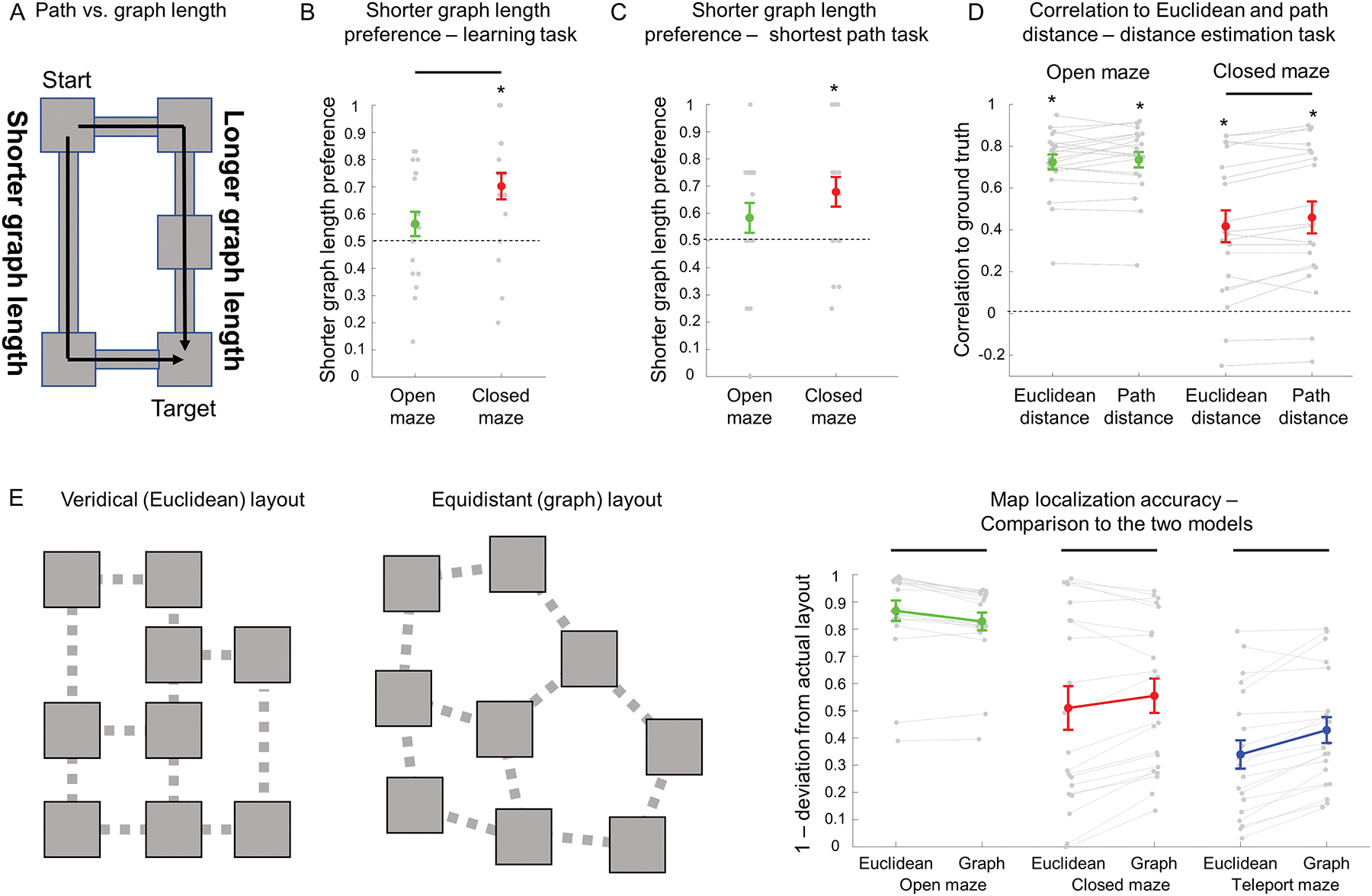
A) A schematic of a sample trial, where there were two pathways between the starting and target objects with equal path length but a different number of intervening rooms (graph length). If participants respond based on Euclidean knowledge alone, then both pathways should be selected with equal probability, but if participants respond based on a cognitive-graph based representation, they would choose the route with fewer intervening rooms because it has shorter graph length. B-C) In the learning task and shortest path selection task, closed-maze participants were biased toward selection of the route with the smaller number of intervening rooms, indicating use of graph knowledge, but open-maze participants were not. D) In the Euclidean distance estimation task, closed-maze participants made estimates that were more highly correlated with path distance than Euclidean distance, indicating a distortion of perceived Euclidean distances by graph knowledge. Open-maze participants did not show this effect. E) In the map localization task, we compared responses to two representational models – one reflecting the Euclidean structure of the environment, the other reflecting the graph structure under the assumption of equal distances between rooms. Reponses of open-maze participants were more consistent with the Euclidean structure of the environment, while responses of closed-maze and teleport-maze participants were more consistent with a cognitive graph representation. Euclidean–veridical Euclidean layout model; Graph – Equidistant graph model. Plot elements are the same as in Figure 2.

In sum, our results suggest that participants’ spatial knowledge extends beyond a Euclidean map and incorporates graph-like elements. Moreover, two of our four analyses show evidence that participants are more likely to use a graph-like code in closed environments compared to open environments, both during navigation in the environment (learning task) and in post-navigation memory tasks.

The structure of the environment affects how spatial knowledge varies across individuals

Finally, we turned to an examination of how spatial knowledge varied across individual participants. Previous work has examined individual differences in cognitive maps within a single environment (Ishikawa & Montello, 2006; Weisberg & Newcombe, 2018), and we wanted to understand how this variability might express itself across different types of environments. To investigate this issue, we focused first on the map localization data, as this is the task that most directly assesses participants’ ability to form an accurate cognitive map of the environment.

Inspection of the data (Fig 4A) revealed an interesting pattern of variability across the three mazes. In the open maze, most participants were able to localize the objects and rooms with high accuracy, but there were two participants who exhibited notably worse performance. In the teleport maze, the converse pattern was observed: most participants were unable to localize the items accurately, but there were participants with notably better performance. This suggests that some teleport maze participants were able to intuit an accurate cognitive map of the environment even in the absence any direct cues about the relative locations of the rooms. Finally, participants in the closed maze showed a wide range of performance, with some participants responding as accurately as the majority of the open maze participants, and some responding as inaccurately as the majority of the teleport maze participants (see Figure S2 for example responses from specific participants).

Figure 4: Individual variability manifests differently across the three environments.

(A) Dot plot of map localization task performance, with k-means clustering into two groups. “Integrators” are participants above the horizontal line and “non-integrators” are participants below the horizontal line. The proportion of integrators varies across environments (almost all participants in the open maze, about half in the closed maze, and almost no participants in the teleport maze), suggesting that the ability to integrate is not a stable personality trait but instead depends on the environment being navigated. (B-E) Spatial memory task performance after dividing participants into “integrators” and “non-integrators” (excluding the small groups of open maze non-integrators and teleport maze integrators). Across tasks, integrators consistently performed better than non-integrators. Moreover, performance of open-maze and closed-maze integrators was similar, as was performance of closed-maze and teleport-maze non-integrators. Plot elements are the same as in Figure 2.

The overall picture suggests that some participants can form an accurate cognitive map, as evidenced by their ability to localize items accurately in the map test, while others cannot, and that this is the case in all three environments but to different degrees. To further examine this idea, we divided participants into two groups using k-means clustering (clustering silhouette score = 0.88, p=0.01). Following the terminology used in Weisberg & Newcombe (Weisberg & Newcombe, 2018), we refer to these two groups as “integrators” (accurate localization) and “non-integrators” (inaccurate localization). These groups were unequally distributed across the three mazes: in the open maze, most participants were integrators; in the closed maze, about half of the participants were integrators and half were non-integrators; in the teleport maze, most participants were non-integrators. The proportion of integrators to non-integrators differed significantly between the mazes (X²(2,n=60)=17.8, p<0.01, Chi-square test). These data support the idea that the propensity of a navigator to behave as an integrator or non-integrator may depend on the structure of the environment.

We next examined the variability of individual performance in the other memory tasks. We were particularly interested in whether the distinction between integrators and non-integrators, derived from map localization performance, would be preserved across tasks. For the statistical analyses, we divided the participants into four groups based on their map localization performance: open maze integrators, closed maze integrators, closed maze non-integrators, and teleport maze non-integrators. We did not analyze open maze non-integrators and teleport maze integrators because there were only small numbers of participants in these groups.

We found that the integrator vs. non-integrator distinction was preserved across all tasks. Performance differed across participant groups in the Euclidean Distance Estimation Task (F(3,49)=40.0, p<0.0001; Fig 4B), the path distance estimation task (F(3,49)=41.5, p<0.0001; Fig 4D) and the shortest path selection task (F(3,49)=46.2, p<0.0001; Fig. 4E). Across these three tasks, performance of closed-maze integrators was significantly better than the performance of closed-maze non-integrators (post-hoc Tukey-Kramer, p<0.0001 in all tasks). In contrast, performance did not differ significantly between open-maze integrators and closed-maze integrators (p>0.91 in all tasks), nor did it differ significantly between closed-maze non-integrators and teleport-maze non-integrators (p>0.26 in all tasks; Table S1). In other words, integrators in the open and closed mazes performed similarly, and non-integrators in the closed and teleport mazes performed similarly. A division between integrators and non-integrators was also observed in the three groups analyzed in the JRD task: performance differed between open-maze integrators, closed-maze integrators, and closed-maze non-integrators (F(2,34)=23.13, p<0.0001; Fig. 4C), and post-hoc pairwise comparison found a significant difference between closed-maze integrators and closed-maze non-integrators (p<0.0001), but not between open-maze integrators and closed-maze integrators (p=0.87).

Bayesian analyses found extremely strong evidence that the integrator and non-integrator groups exhibited different levels of performance in all tasks (e.g., BF10s>800 for integrator vs. non-integrator the closed maze; Table S1). However, there was only weak evidence for the null hypotheses that open-maze integrators and closed-maze integrators had the same performance (BF10s=0.40–0.51) and that closed-maze non-integrators and teleport-maze non-integrators had the same performance (BF10s=0.38–0.71). The latter results indicate that we cannot make strong claims that performance is driven entirely by integrator vs. non-integrator status—the structure of the environment may have an additional influence beyond its effect on the assignment of individuals to these groups.

To explore the type of representation formed by integrators and non-integrators, we focused on the closed maze participants and examined their map localization responses. As in the previous section, we compared responses to the Euclidean structure of the space and an equidistant graph model, but this time looking at integrators and non-integrators separately. This analysis revealed that maps produced by integrators exhibited a greater resemblance to the Euclidean structure of the space (marginal effect, p=0.07), whereas maps produced by non-integrators showed a greater resemblance to the equidistant graph model (p<0.0001), with the difference between the two groups being significant (p<0.0001; Figure 5, Table S1). These findings suggest that integrators tend to form Euclidean representations in the closed maze, akin to participants in the open maze, whereas non-integrators tend to form graph-like representations, similar to participants in the teleport maze.

Figure 5: Integrators form Euclidean representations, whereas non-integrators form graph-like representations.

The plot indicates the fit of the map localization responses of integrators and non-integrators to two representational models (Euclidean or graph; see Figure 3E). Open-maze and closed-maze integrators use a veridical Euclidean representation of the space, whereas closed-maze and teleport maze non-integratorsuse a graph-like representation. Plot elements are the same as in Figure 2.

What drives the division of participants into integrators and non-integrators? Our findings suggest that the environment itself is a primary factor: most participants in the open maze are integrators, whereas most participants in the teleport maze are non-integrators. However, the fact that individual differences are observed in all three environments indicates that the effect of the environment is not absolute. To explore potential factors related to this within-environment individual variability, we examined its relation to participants’ baseline spatial abilities, including perspective-taking ability (PTTA score) and self-rated navigational ability (SBSOD score), as well as their sex, by comparing these factors between integrators and non-integrators in the closed maze. We found that integrators had higher SBSOD and PTTA scores than non-integrators (t(18)=2.22, 2.22, both ps=0.04), and that integrators were significantly more likely to be male (t(18)=2.48, p=0.04; two-tailed two-sample t-tests, FDR corrected across measures; Fig. 6).

Figure 6: Sex, SBSOD and PTTA differences between integrators and non-integrators in the closed maze.

Plot elements are the same as in Figure 2.

We then examined the correlation between these factors (SBSOD, PTTA, sex) and performance in specific tasks within each maze, in this case collapsing over the integrator/non-integrator distinction (Table S2). We did not observe any relationships in the open or teleport mazes, most likely because variability of performance in these mazes was not sufficient to observe significant effects. In the open maze, male sex was significantly correlated with performance in the Euclidean distance estimation, path distance estimation, shortest path selection, map localization, and JRD (all ps<0.05; FDR-corrected across tasks and environmental conditions). Correlations between participants’ PTTA and SBSOD scores and their performance in the specific tasks were positive but did not reach significance after multiple correction over maze and task. Overall, our results suggest that within-environment variability in environmental learning is related to participants’ baseline navigation and perspective taking ability, as well as to their sex.

In summary, our findings indicate that the environment plays a crucial role in dividing participants into integrators and non-integrators. Most participants perform well in open environments, and most perform poorly in cue-limited (teleport maze) environments. Variability between individuals becomes most pronounced in maze-like environments, which have limited visibility and require the internal tracking of location and direction.

Discussion

The aim of this study was to understand how the physical structure of the navigable environment affects the accuracy and format of cognitive maps. Our analyses yielded three main findings. First, the accuracy of spatial knowledge was affected by the structure of the environment. Despite the fact that the open maze, closed maze, and teleport maze all had the same number of rooms and the same connectivity structure, spatial memory differed substantially between these conditions, with greater accuracy in environments with greater number of orienting cues (open>closed>teleport). Second, the format of spatial knowledge was also affected by the structure of the environment. Although we found evidence for both map-like and graph-like representations, participants used graph-like codes more often in the closed and teleport mazes compared to the open maze. Third, inter-individual variability in spatial knowledge was affected by the structure of the environment. Variability was relatively low in the open maze, where most participants were classified as integrators, and it was also low in the teleport maze, where most participant were classified as non-integrators. In contrast, variability was higher in the closed maze, where participants fell about evenly into these two groups. Notably, we found that non-integrators in the closed maze represented the maze as resembling an equidistant graph, while the representations of integrators were more similar the actual Euclidean distances between locations. Taken together, these results emphasize the strong effect that environmental structure has on spatial knowledge, and indicate that past and future studies of spatial representations should be carefully interpreted with respect to the specific type of environment used in each study. Below we discuss each of our main findings in more detail.

The first question we asked was whether the structure of the environment affects the accuracy of spatial knowledge. We found strong evidence that it does. There was a consistent ordering of performance across the environments: accuracy in all of our spatial memory tasks was highest for participants in the open maze, intermediate for participants in the closed maze, and lowest for participants in the teleport maze. This was despite the fact that all three environments had the exact same number of rooms, room geometry, and connectivity structure.

What could be the cause of this ordering? By design, the three environments differed in the cues available for determining heading and location in global Euclidean space. In the open maze, the entire environment was always visible, including the boundary of the courtyard and the distal landmarks. Thus, it was possible for participants to determine their global location and heading directly through perception. In the closed maze, on the other hand, participants could not see beyond the walls that bounded the local room or corridor. Thus, they could determine their local (within-room) location and heading through direct perception, but their global position and heading could only be ascertained by using an active memory process to keep track of these quantities as they moved from room to room. In the teleport maze, even this active tracking process was not possible, because there were no distance cues when participants were teleported from room to room, and their heading when placed in the new room was randomly chosen. Thus, the key factor that likely accounts for the difference in performance across the three environments is the ability of the participants to maintain a sense of global location and direction in Euclidean space during learning. This conclusion is consistent with a large literature that suggests that the ability to path integrate—to keep track of one’s position and heading during exploration—is crucial for building up a cognitive map (Etienne & Jeffery, 2004; McNaughton et al., 1996, 2006).

The second question that we asked was whether the format of the environment affects the format of the cognitive map. The question of format has been the subject of considerable ongoing debate. Some theories posit that spatial knowledge consists of a map of locations represented within a global Euclidean coordinate system (Gallistel, 1990; O’Keefe & Nadel, 1978; Siegel & White, 1975), while others theories posit that it consists of a graph of routes connecting different locations, with no integration of the locations into a single global reference frame (Kuipers, 1982; Meilinger, 2008; Warren, 2019). In a previous review, we argued that map-like and graph-like representations might simultaneously exist in the same individuals and be differentially employed in different environments (Peer et al., 2021). Our findings provide evidence in support of these ideas.

Consideration of results across the three environments suggests that people formed both Euclidean and graph-like representations. Supporting the use of Euclidean codes is the fact that participants were able to perform tasks that were designed to tap Euclidean knowledge (map localization, Euclidean distance estimation, JRD). Moreover—as discussed in the previous section—their ability to do so varied across environments depending on the presence or absence of cues that allowed them to determine their global Euclidean position and heading. Of particular note, the difference in performance between the open and closed maze would not be found if only graph-like representations were formed, because such representations only encode local spatial features (node identity, angle of links at a node) that are equally present in both the open and closed maze (Ericson & Warren, 2020; Warren, 2019). However, we also found evidence for graph-like representations. Participants’ navigational choices during learning and their responses in the shortest path task were influenced by graph knowledge: when faced with a decision between two paths of equal Euclidean length in the open and closed mazes, they preferred the path with fewer graph segments. Moreover, their Euclidean distance estimates in the closed maze were more highly correlated to path distances than to Euclidean distances, suggesting that a graph-like representation was accessed during this task. Finally, the mere fact that participants were able to navigate accurately in the teleport maze where only connectivity information was available suggests that spatial representations can, in some circumstances, be predominantly graph-based. Thus, neither Euclidean maps nor cognitive graphs can explain our results on their own; both are needed.

We also found some support for the idea that the use of graph knowledge would vary across environments depending on their structure. When navigating through the environment in the learning phase, participants in the closed maze exhibited a stronger preference for paths with fewer graph segments (when presented with alternatives of equal length) compared to participants in the open maze. Furthermore, in the map localization task, participants in the teleport maze, as well as non-integrators in the closed maze, demonstrated memory of object locations that aligned more closely with an equidistant graph-like representation than with the Euclidean layout of the environment. In contrast, participants in the open maze, as well as integrators in the closed maze, exhibited memory that more closely resembled the Euclidean layout of the environment. These findings support our previous suggestion that the challenge of integrating subspaces into a global Euclidean representation within a closed environment may lead to greater reliance on environmental topology, resulting in the formation of a graph-like representation (Peer et al., 2021). .

The final question that we asked was how individual variability would manifest across the three environments. Previous reports have demonstrated marked differences between people in their ability to integrate subparts of the environment to form a global cognitive map (e.g. (Ishikawa & Montello, 2006; Weisberg et al., 2014; Weisberg & Newcombe, 2018)). For example, in an environment consisting of constrained routes, people can be separated into three groups: integrators, who can accurately point to locations in separately-learned parts of the environment; non-integrators, who can point to locations in the same part of the environment but cannot point across parts; and imprecise navigators, who cannot accurately point to any location (Ishikawa & Montello, 2006; Weisberg et al., 2014; Weisberg & Newcombe, 2018). These differences have been shown to relate both to general cognitive abilities like mental rotation and perspective taking (Weisberg et al., 2014), as well as to the type of environment people grew up in (e.g. the layout of streets in people’s home town (Barhorst-Cates et al., 2021; Coutrot et al., 2022)). However, these studies all used a single environment, leaving open the question of whether the observed individual differences are stable character traits, or—alternatively—tendencies that might manifest differently in the same individual depending on environmental context.

Here we found that there was a strong interaction between individuals’ cognitive mapping ability and the structure of the environment: in the open maze most participants were integrators, in the teleport maze most participants were non-integrators, and in the closed maze participants fell about equally into the two groups. But there were some notable exceptions: some participants performed poorly in the open maze despite the abundance of spatial cues, and some participants performed well in the teleport maze (even in the Euclidean tasks), despite a paucity of cues. These results suggest that cognitive mapping ability manifests differently across environments in most people, but there are some individuals on the extreme ends of the spectrum who show a greater degree of stability in their performance. Additionally, our results provide evidence that non-integrators, who face difficulties in estimating Euclidean distances and relations, are more likely than integrators to represent the environment in a graph-like format.

Previous studies of individual differences in cognitive mapping have used environments that allowed continuous tracking of location and heading, but without full visibility to other parts of the environment (Ishikawa & Montello, 2006; Weisberg & Newcombe, 2018). The variability observed in these studies might be less robust in more open environments, or in unusually restricted environments like our teleport maze. Furthermore, the ability to mentally track location and heading might depend on perspective taking ability, which we found to be correlated to the individual differences in our task, in line with previous studies (Allen et al., 1996; Fields & Shelton, 2006; Kozhevnikov et al., 2006; Schinazi et al., 2013). The interaction we observed between individual variability and environmental features is in line with a recent study which found that the existence of orienting landmarks interacts with individual variability in navigation, and that this variability is correlated to individuals’ sex, mental rotation ability and perspective taking ability (Cherep et al., 2023). Overall, this set of findings has two major implications: first, past (and future) studies of variability in navigational ability should be carefully interpreted with respect to the specific environment being explored; and second, specific environmental features can reduce the variability between people and allow some “bad navigators” to navigate efficiently and integrate between different environmental subparts, suggesting implications for real-life environmental design.

In conclusion, we found that specific features of each environment affect the accuracy and format of the mental representations people form of these environments. We further found that individual variability in cognitive map formation and use of graph knowledge are not constant but instead depend on the environment being learned. These findings suggest that care should be taken to consider the specific environment’s features when interpreting the spatial navigation literature, and that environments and navigational aids can be designed to facilitate navigation even for people who would otherwise be bad navigators.

Constraints on Generality

Our study has several limitations. First, we used environments that differed from each other along more than one feature (e.g. the open maze differed from the closed maze both in visibility across the environment and in the existence of distal landmarks). Further studies might attempt to disentangle the effect of each of these features on the resulting spatial representations, and test how the observed effects generalize to other environments. Second, our study did not investigate within-subject effects – although our individual difference analyses suggest that some individuals would perform differently in different environments, we do not have direct evidence that this is the case. Third, the study population was predominantly young adults, many of whom were university students, and participants were educated members of western societies who are familiar with built urban environments (e.g. cities with rectilinear streets, buildings with corridors and rooms). Further studies are needed to confirm the generality of the findings for other age groups and population sectors, and for human populations whose primary experience is with natural environments. Fourth, there are several important dimensions of environmental organization that we did not examine, such as division of the environment into segments that may be hierarchically organized (Hirtle & Jonides, 1985; McNamara et al., 1989). It is possible that our participants formed such representations in the present environments, but in an idiosyncratic manner that varied across individuals, thus making them difficult to test. Finally, some features of our environments (e.g. teleportation in the teleport maze, and virtual desktop navigation) are not realistic; future studies may study how these effects are manifested in real-life environments.

Public Significance statement.

This study shows that people form different types of mental maps of different types of spaces. If the space being learned is open, people are likely to form a mental map that has information about the straight-line distances and directions between different locations. In contrast, if the space has limited visibility between its parts (e.g. a maze), people are likely to form a mental map that has information about the routes that connect different places (“cognitive graph”), and less about their exact locations. These findings illuminate how people create mental representations of different physical spaces, and may have implications about how they learn abstract spaces.

References

- Allen GL, Kirasic KC, Dobson SH, Long RG, & Beck S (1996). Predicting environmental learning from spatial abilities: An indirect route. Intelligence, 22(3), 327–355. 10.1016/S0160-2896(96)90026-4 [DOI] [Google Scholar]
- Barhorst-Cates EM, Meneghetti C, Zhao Y, Pazzaglia F, & Creem-Regehr SH (2021). Effects of home environment structure on navigation preference and performance: A comparison in Veneto, Italy and Utah, USA. Journal of Environmental Psychology, 74, 101580. 10.1016/j.jenvp.2021.101580 [DOI] [Google Scholar]
- Chadwick MJ, Jolly AEJ, Amos DP, Hassabis D, & Spiers HJ (2015). A Goal Direction Signal in the Human Entorhinal/Subicular Region. Current Biology, 25(1), 87–92. 10.1016/j.cub.2014.11.001 [DOI] [PMC free article] [PubMed] [Google Scholar]
- Cherep LA, Kelly JW, Miller A, Lim AF, & Gilbert SB (2023). Individual differences in teleporting through virtual environments. Journal of Experimental Psychology: Applied, 29(1), 111–123. 10.1037/xap0000396 [DOI] [PubMed] [Google Scholar]
- Chrastil ER, & Warren WH (2014). From cognitive maps to cognitive graphs. PloS One, 9(11), e112544. [DOI] [PMC free article] [PubMed] [Google Scholar]
- Coutrot A, Manley E, Goodroe S, Gahnstrom C, Filomena G, Yesiltepe D, Dalton RC, Wiener JM, Hölscher C, Hornberger M, & Spiers HJ (2022). Entropy of city street networks linked to future spatial navigation ability. Nature, 604(7904), 104–110. 10.1038/s41586-022-04486-7 [DOI] [PubMed] [Google Scholar]
- Doeller CF, Barry C, & Burgess N (2010). Evidence for grid cells in a human memory network. Nature, 463(7281), 657–661. 10.1038/nature08704 [DOI] [PMC free article] [PubMed] [Google Scholar]
- Doner S, Zheng J, McAvan AS, Starrett MJ, Campbell H, Sanders D, & Ekstrom A (2022). Evidence for flexible navigation strategies during spatial learning involving path choices. Spatial Cognition & Computation, 1–30. 10.1080/13875868.2022.2158090 [DOI] [Google Scholar]
- Ericson JD, & Warren WH (2020). Probing the invariant structure of spatial knowledge: Support for the cognitive graph hypothesis. Cognition, 200, 104276. 10.1016/j.cognition.2020.104276 [DOI] [PubMed] [Google Scholar]
- Etienne AS, & Jeffery KJ (2004). Path integration in mammals. Hippocampus, 14(2), 180–192. 10.1002/hipo.10173 [DOI] [PubMed] [Google Scholar]
- Faul F, Erdfelder E, Buchner A, & Lang A-G (2009). Statistical power analyses using G*Power 3.1: Tests for correlation and regression analyses. Behavior Research Methods, 41(4), 1149–1160. 10.3758/BRM.41.4.1149 [DOI] [PubMed] [Google Scholar]
- Fields AW, & Shelton AL (2006). Individual skill differences and large-scale environmental learning. Journal of Experimental Psychology: Learning, Memory, and Cognition, 32(3), 506–515. 10.1037/0278-7393.32.3.506 [DOI] [PubMed] [Google Scholar]
- Frick A, Möhring W, & Newcombe NS (2014). Picturing perspectives: Development of perspective-taking abilities in 4- to 8-year-olds. Frontiers in Psychology, 5. 10.3389/fpsyg.2014.00386 [DOI] [PMC free article] [PubMed] [Google Scholar]
- Gallistel CR (1990). The organization of learning (pp. viii, 648). The MIT Press. [Google Scholar]
- He Q, & Brown TI (2019). Environmental Barriers Disrupt Grid-like Representations in Humans during Navigation. Current Biology, 29(16), 2718–2722.e3. 10.1016/j.cub.2019.06.072 [DOI] [PMC free article] [PubMed] [Google Scholar]
- Hegarty M (2002). Development of a self-report measure of environmental spatial ability. Intelligence, 30(5), 425–447. 10.1016/S0160-2896(02)00116-2 [DOI] [Google Scholar]
- Hirtle SC, & Jonides J (1985). Evidence of hierarchies in cognitive maps. Memory & Cognition, 13(3), 208–217. 10.3758/BF03197683 [DOI] [PubMed] [Google Scholar]
- Ishikawa T, & Montello D (2006). Spatial knowledge acquisition from direct experience in the environment: Individual differences in the development of metric knowledge and the integration of separately learned places☆. Cognitive Psychology, 52(2), 93–129. 10.1016/j.cogpsych.2005.08.003 [DOI] [PubMed] [Google Scholar]
- Jacobs J, Weidemann CT, Miller JF, Solway A, Burke JF, Wei X-X, Suthana N, Sperling MR, Sharan AD, Fried I, & Kahana MJ (2013). Direct recordings of grid-like neuronal activity in human spatial navigation. Nature Neuroscience, 16(9), 1188–1190. 10.1038/nn.3466 [DOI] [PMC free article] [PubMed] [Google Scholar]
- Kamada T, & Kawai S (1989). An algorithm for drawing general undirected graphs. Information Processing Letters, 31(1), 7–15. 10.1016/0020-0190(89)90102-6 [DOI] [Google Scholar]
- Kozhevnikov M, Motes MA, Rasch B, & Blajenkova O (2006). Perspective-taking vs. Mental rotation transformations and how they predict spatial navigation performance. Applied Cognitive Psychology, 20(3), 397–417. 10.1002/acp.1192 [DOI] [Google Scholar]
- Krekelberg B (2022). A Matlab toolbox for Bayes Factor statistical analysis (v2.3.0). Zenodo. 10.5281/ZENODO.4394422 [DOI] [Google Scholar]
- Kuipers B (1982). The “Map in the Head” Metaphor. Environment and Behavior, 14(2), 202–220. 10.1177/0013916584142005 [DOI] [Google Scholar]
- Maidenbaum S, Miller J, Stein JM, & Jacobs J (2018). Grid-like hexadirectional modulation of human entorhinal theta oscillations. Proceedings of the National Academy of Sciences, 115(42), 10798–10803. 10.1073/pnas.1805007115 [DOI] [PMC free article] [PubMed] [Google Scholar]
- Marchette SA, Ryan J, & Epstein RA (2017). Schematic representations of local environmental space guide goal-directed navigation. Cognition, 158, 68–80. 10.1016/j.cognition.2016.10.005 [DOI] [PMC free article] [PubMed] [Google Scholar]
- McNamara TP, Hardy JK, & Hirtle SC (1989). Subjective hierarchies in spatial memory. Journal of Experimental Psychology: Learning, Memory, and Cognition, 15(2), 211–227. 10.1037/0278-7393.15.2.211 [DOI] [PubMed] [Google Scholar]
- McNaughton BL, Barnes CA, Gerrard JL, Gothard K, Jung MW, Knierim JJ, Kudrimoti H, Qin Y, Skaggs WE, Suster M, & Weaver KL (1996). Deciphering the hippocampal polyglot: The hippocampus as a path integration system. Journal of Experimental Biology, 199(1), 173–185. 10.1242/jeb.199.1.173 [DOI] [PubMed] [Google Scholar]
- McNaughton BL, Barnes CA, & O’Keefe J (1983). The contributions of position, direction, and velocity to single unit activity in the hippocampus of freely-moving rats. Experimental Brain Research, 52(1). 10.1007/BF00237147 [DOI] [PubMed] [Google Scholar]
- McNaughton BL, Battaglia FP, Jensen O, Moser EI, & Moser M-B (2006). Path integration and the neural basis of the “cognitive map.” Nature Reviews Neuroscience, 7(8), Article 8. 10.1038/nrn1932 [DOI] [PubMed] [Google Scholar]
- Mehta MR, Barnes CA, & McNaughton BL (1997). Experience-dependent, asymmetric expansion of hippocampal place fields. Proceedings of the National Academy of Sciences, 94(16), 8918–8921. 10.1073/pnas.94.16.8918 [DOI] [PMC free article] [PubMed] [Google Scholar]
- Meilinger T (2008). The Network of Reference Frames Theory: A Synthesis of Graphs and Cognitive Maps. In Freksa C, Newcombe NS, Gärdenfors P, & Wölfl S (Eds.), Spatial Cognition VI. Learning, Reasoning, and Talking about Space (pp. 344–360). Springer. 10.1007/978-3-540-87601-4_25 [DOI] [Google Scholar]
- Miller JF, Lazarus EM, Polyn SM, & Kahana MJ (2013). Spatial clustering during memory search. Journal of Experimental Psychology: Learning, Memory, and Cognition, 39(3), 773–781. 10.1037/a0029684 [DOI] [PMC free article] [PubMed] [Google Scholar]
- Moeser SD (1988). Cognitive Mapping in a Complex Building. Environment and Behavior, 20(1), 21–49. 10.1177/0013916588201002 [DOI] [Google Scholar]
- Moser EI, Kropff E, & Moser M-B (2008). Place Cells, Grid Cells, and the Brain’s Spatial Representation System. Annual Review of Neuroscience, 31(1), 69–89. 10.1146/annurev.neuro.31.061307.090723 [DOI] [PubMed] [Google Scholar]
- Mou W, & Wang L (2015). Piloting and path integration within and across boundaries. Journal of Experimental Psychology: Learning, Memory, and Cognition, 41(1), 220–234. 10.1037/xlm0000032 [DOI] [PubMed] [Google Scholar]
- Muller R, Bostock E, Taube J, & Kubie J (1994). On the directional firing properties of hippocampal place cells. The Journal of Neuroscience, 14(12), 7235–7251. 10.1523/JNEUROSCI.14-12-07235.1994 [DOI] [PMC free article] [PubMed] [Google Scholar]
- Muryy A, & Glennerster A (2018). Pointing Errors in Non-metric Virtual Environments. In Creem-Regehr S, Schöning J, & Klippel A (Eds.), Spatial Cognition XI (pp. 43–57). Springer International Publishing. 10.1007/978-3-319-96385-3_4 [DOI] [Google Scholar]
- O’Keefe J, & Dostrovsky J (1971). The hippocampus as a spatial map. Preliminary evidence from unit activity in the freely-moving rat. Brain Research, 34(1), 171–175. 10.1016/0006-8993(71)90358-1 [DOI] [PubMed] [Google Scholar]
- O’Keefe J, & Nadel L (1978). The Hippocampus as a Cognitive Map. Oxford: Clarendon Press. https://repository.arizona.edu/handle/10150/620894 [Google Scholar]
- Peer M, Brunec IK, Newcombe NS, & Epstein RA (2021). Structuring Knowledge with Cognitive Maps and Cognitive Graphs. Trends in Cognitive Sciences, 25(1), 37–54. 10.1016/j.tics.2020.10.004 [DOI] [PMC free article] [PubMed] [Google Scholar]
- Peer M, & Epstein RA (2021). The human brain uses spatial schemas to represent segmented environments. Current Biology, 31(21), 4677–4688.e8. 10.1016/j.cub.2021.08.012 [DOI] [PMC free article] [PubMed] [Google Scholar]
- Schinazi VR, Nardi D, Newcombe NS, Shipley TF, & Epstein RA (2013). Hippocampal size predicts rapid learning of a cognitive map in humans. Hippocampus, 23(6), 515–528. 10.1002/hipo.22111 [DOI] [PMC free article] [PubMed] [Google Scholar]
- Shannon P, Markiel A, Ozier O, Baliga NS, Wang JT, Ramage D, Amin N, Schwikowski B, & Ideker T (2003). Cytoscape: A software environment for integrated models of biomolecular interaction networks. Genome Research, 13(11), 2498–2504. 10.1101/gr.1239303 [DOI] [PMC free article] [PubMed] [Google Scholar]
- Shine JP, Valdés-Herrera JP, Tempelmann C, & Wolbers T (2019). Evidence for allocentric boundary and goal direction information in the human entorhinal cortex and subiculum. Nature Communications, 10(1), 4004. 10.1038/s41467-019-11802-9 [DOI] [PMC free article] [PubMed] [Google Scholar]
- Siegel AW, & White SH (1975). The Development of Spatial Representations of Large-Scale Environments. In Reese HW (Ed.), Advances in Child Development and Behavior (Vol. 10, pp. 9–55). JAI. 10.1016/S0065-2407(08)60007-5 [DOI] [PubMed] [Google Scholar]
- Van Doorn J, Van Den Bergh D, Böhm U, Dablander F, Derks K, Draws T, Etz A, Evans NJ, Gronau QF, Haaf JM, Hinne M, Kucharský Š, Ly A, Marsman M, Matzke D, Gupta ARKN, Sarafoglou A, Stefan A, Voelkel JG, & Wagenmakers E-J (2021). The JASP guidelines for conducting and reporting a Bayesian analysis. Psychonomic Bulletin & Review, 28(3), 813–826. 10.3758/s13423-020-01798-5 [DOI] [PMC free article] [PubMed] [Google Scholar]
- Warren WH (2019). Non-Euclidean navigation. Journal of Experimental Biology, 222(Suppl 1). 10.1242/jeb.187971 [DOI] [PubMed] [Google Scholar]
- Weisberg SM, & Newcombe NS (2018). Cognitive Maps: Some People Make Them, Some People Struggle. Current Directions in Psychological Science, 27(4), 220–226. 10.1177/0963721417744521 [DOI] [PMC free article] [PubMed] [Google Scholar]
- Weisberg SM, Schinazi VR, Newcombe NS, Shipley TF, & Epstein RA (2014). Variations in cognitive maps: Understanding individual differences in navigation. Journal of Experimental Psychology: Learning, Memory, and Cognition, 40(3), 669–682. 10.1037/a0035261 [DOI] [PubMed] [Google Scholar]
- Zetzsche C, Wolter J, Galbraith C, & Schill K (2009). Representation of space: Image-like or sensorimotor? Spatial Vision, 22(5), 409–424. 10.1163/156856809789476074 [DOI] [PubMed] [Google Scholar]
Associated Data
This section collects any data citations, data availability statements, or supplementary materials included in this article.