American Society of Anesthesiologists Physical Status Classification Significantly Affects the Performances of Machine Learning Models in Intraoperative Hypotension Inference

Abstract

Study Objective:

To explore how American Society of Anesthesiologists (ASA) physical status classification affects different machine learning models in hypotension prediction and whether the prediction uncertainty could be quantified.

Design:

Observational Studies

Setting:

UofL health hospital

Patients:

This study involved 562 hysterectomy surgeries performed on patients (≥ 18 years) between June 2020 and July 2021.

Interventions:

None

Measurements:

Preoperative and intraoperative data is collected. Three parametric machine learning models, including Bayesian generalized linear model (BGLM), Bayesian neural network (BNN), a newly proposed BNN with multivariate mixed responses (BNNMR), and one nonparametric model, Gaussian Process (GP), were explored to predict patients’ diastolic and systolic blood pressures (continuous responses) and patients’ hypotensive event (binary response) for the next five minutes. Data was separated into American Society of Anesthesiologists (ASA) physical status class 1~'4 before being read in by four machine learning models. Statistical analysis and models’ constructions are performed in Python. Sensitivity, specificity, and the confidence/credible intervals were used to evaluate the prediction performance of each model for each ASA physical status class.

Main Results:

ASA physical status classes require distinct models to accurately predict intraoperative blood pressures and hypotensive events. Overall, high sensitivity (above 0.85) and low uncertainty can be achieved by all models for ASA class 4 patients. In contrast, models trained without controlling ASA classes yielded lower sensitivity (below 0.5) and larger uncertainty. Particularly, in terms of predicting binary hypotensive event, for ASA physical status class 1, BNNMR yields the highest sensitivity of 1. For classes 2 and 3, BNN has the highest sensitivity of 0.429 and 0.415, respectively. For class 4, BNNMR and GP are tied with the highest sensitivity of 0.857. On the other hand, the sensitivity is just 0.031, 0.429, 0.165 and 0.305 for BNNMR, BNN, GBLM and GP models respectively, when training data is not divided by ASA physical status classes. In terms of predicting systolic blood pressure, the GP regression yields the lowest root mean squared errors (RMSE) of 2.072, 7.539, 9.214 and 0.295 for ASA physical status classes 1, 2, 3 and 4, respectively, but a RMSE of 126.894 if model is trained without controlling the ASA physical status class. The RMSEs for other models are far higher. RMSEs are 2.175, 13.861, 17.560 and 22.426 for classes 1, 2, 3 and 4 respectively for the BGLM. In terms of predicting diastolic blood pressure, the GP regression yields the lowest RMSEs of 2.152, 6.573, 5.371 and 0.831 for ASA physical status classes 1, 2, 3 and 4, respectively; RMSE of 8.084 if model is trained without controlling the ASA physical status class. The RMSEs for other models are far higher. Finally, in terms of the width of the 95% confidence interval of the mean prediction for systolic and diastolic blood pressures, GP regression gives narrower confidence interval with much smaller margin of error across all four ASA physical status classes.

Conclusions:

Different ASA physical status classes present different data distributions, and thus calls for distinct machine learning models to improve prediction accuracy and reduce predictive uncertainty. Uncertainty quantification enabled by Bayesian inference provides valuable information for clinicians as an additional metric to evaluate performance of machine learning models for medical decision making.

Introduction

In recent years, machine learning has been widely applied to predict medical outcomes such as blood pressure [1–4], postoperative mortality [5], acute kidney injury [6], and reintubation [6]. Commonly used algorithms consist of Recurrent Neural Networks (RNN), Deep Neural Networks (DNN), Convolutional Neural Network (CNN), and Multipath CNN. However, significant gaps still exist between these predictive tools and clinical applications by anesthesiologists. Intraoperative hypotension is common during surgery and has been associated with postoperative kidney injury, ischemic strokes, ultimately leading to an eightfold increase in postoperative mortality [7–11]. Contributing factors to intraoperative hypotension include anesthetic drugs, surgical blood loss, patient co-morbidities, medications, patient positioning, and compression of major vessels. This paper aims to predict intraoperative hypotension within a reasonable time (e.g., 5 minutes) to proactively manage pending hypotension.

In the past decades, many signal processing and machine learning methods have been developed to predict hypotension or blood pressure in order to understand the root causes of hypotension and thus to proactively manage resulting complications. However, there are still three major research gaps. First, most of existing methods are designed for point prediction, which only provide the predicted mean values of either the probability of hypotension or blood pressures. Without the uncertainty quantification of such mean values (i.e., interval estimation which identifies the degree to which a prediction model is uncertain), the decision maker’s trust of the prediction cannot be easily built. Second, most existing machine learning models assume that samples from electronic medical records are independently and identically distributed (i.i.d.) for the variables of interest. However, this assumption does not hold in practical datasets. In fact, large heterogeneities exist in the datasets with medical records, due to wide range of demographics, medical history, health conditions of different patients. These heterogeneities can easily fail a well-trained machine learning model. Researchers and practitioners generally adopted clustering methods to separate samples into different clusters and fit different models within each cluster. However, no standard has been established for clustering, hence causing difficulties for these models to be widely adopted. Third, hypotensive event as a binary response and blood pressures as continuous responses are usually modeled separately without consideration of their hidden correlations. However, the binary hypotension classification is inherently correlated with the decrement in blood pressures. Such correlation suggests that sharing information among binary and continuous responses may regularize machine learning model to prevent unreasonable predictions, as well as enhance the accuracy of the predictions.

To address these research gaps, we explored Bayesian Neural Network (BNN), Gaussian Process (GP), and Bayesian Generalized Linear Models (BGLM) to predict the systolic and diastolic blood pressures (continuous response) and intraoperative hypotension event (binary response) on four datasets, divided by patients’ ASA physical status classification 1~'4. We also build the BNN with multivariate Mixed Response (BNNMR) to jointly predict the blood pressure and binary outcome [12]. Finally, unlike most literature that uses either mean or lastly observed values [1–6], we use the principal component analysis (PCA) to fill in the missing values in our dataset, a common issue to address in data analytics for clinical research due to high level of heterogeneity among patients and their health conditions [13].

Materials and Methods

Data Source and Study Approval

Data was collected from 562 hysterectomy surgeries performed on patients (≥ 18 years) between June 2020 and July 2021 at University of Louisville Health, Louisville, KY, USA. Hysterectomy surgery was selected because they are standardized and well controlled procedures. This study was approved by the University of Louisville (UofL) Institutional Review Board (Study No. 20.0969) and by UofL Health for legal and privacy compliance.

Data Preprocessing

We first address the data incompleteness based on a two-step approach. First, we utilize the principal component analysis (PCA) with the expectation maximization algorithm to impute the missing values in input variables [14, 15]. Second, we define the sample by utilizing a sliding-window based strategy due to the block missing values, which are caused by inconsistent sampling rates (see empty cells in Figure 1). A sliding window is a technique used in time series analysis and signal processing [16]. Imagine a fixed size “window” that captures a specific segment of the data, and this window “slides” over the data to capture the next segment. By moving the window across the data with a fixed increment, we can transform a continuous or long series of data into smaller, overlapping or non-overlapping chunks [16]. Specifically, a one-step-ahead strategy is proposed to construct a sliding window to predict the next observed responses. The window size is 30 minutes as a consolidation of raw data in six 5-minute sessions. For example, the seventh row in Fig. 1 is the result of the consolidation of the six immediately preceding rows and will be counted as one sample. This consolidation starts with the first blood pressure reading after the first six input variable readings and continues through the last blood pressure reading. By sliding the window across the entire time series (from the beginning of a surgery till the end) of data for each patient, multiple samples per patient are generated. Consequently, the sample size of the processed dataset is a function of the number of patients and the number of time intervals for which patients have valid records. Our final dataset contains 7,177 samples for 562 patients/cases. These 7,177 samples are divided into four clusters: ASA Class 1 (n = 144), ASA Class 2 (n = 2680), ASA Class 3 (n = 3952) and ASA Class 4 (n = 401). Using sliding windows in time series analysis captures data within its crucial temporal context, preserving the order and relationships between data points. This method offers flexibility, allowing adjustments in granularity by changing window or step sizes. It addresses issues in datasets with rare significant events by reducing temporal sparsity, especially when windows overlap. Moreover, sliding windows provide a uniform data structure, ideal for consistent analysis and modeling, particularly in deep learning. This comprehensive view ensures no event or change goes unnoticed, making the representation rich and potentially capturing all relevant variations in the data [16, 17].

Figure 1. An example of a one-step-ahead prediction strategy:

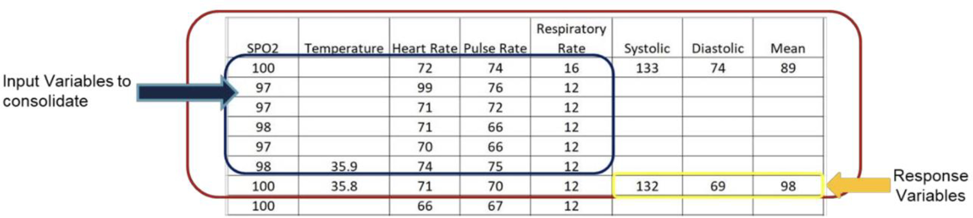
each row represents a 5-minute interval, one sample is defined as six rows of input variables and one row of response variables.

77 input variables are extracted to build prediction models. Among them, 30 are preoperative variables, and 47 are intraoperative variables. Particularly, ‘Hypotension’ (binary), ‘Systolic Blood Pressure’ (continuous), and ‘Diastolic Blood Pressure’ (continuous) are the mixed responses. We conduct a stratified 5-fold cross validation to split the training and testing datasets to ensure that no class will be underrepresented. Such technique divides each dataset into 5 folds while maintaining the original ASA class distribution in each fold. This method also ensures both training and testing sets have consistent class proportions. Then the standardization is applied, so that all variables have zero-mean and unit variance. (Detailed list of variables are available in Table S1 under Supplementary Materials.)

Our dataset of 7177 samples from 562 patients is a true representation of diverse ASA classes and has undergone rigorous validation. Each case was reviewed by two anesthesiologists independently to ensure the accuracy of ASA classifications.

Model Categorization

We examined both parametric and non-parametric models [18]. Parametric models assume a specific probability distribution for the data, while nonparametric models make little or no assumptions about the distribution. Comparing the performance of both models on the same dataset helps us understand whether the data follows the assumed distribution or not. In our case, parametric would assume data follows Gaussian distribution, hence we adopt two models. One is a parsimonious model, i.e., Bayesian Generalized Linear Regression Model (BGLM). The BGLM selects the most important predictors to achieve balance between model complexity and predictive. Under the BGLM, we use Bayesian Ridge Regression to predict blood pressures, and Bayesian Logistic Regression to predict binary hypotension index. The second parametric model is the Bayesian Neural Network (BNN). The BNN captures the nonlinear input-output relationship and uses Bayesian inference to model uncertainty associated with model coefficients. The other class of models we study is the non-parametric model, more specifically the Gaussian Process (GP). In general, GP’s prior is defined by a mean function and a covariance function, which does not depend on any specific set of parameters.

Bayesian Neural Network

BNN advances the standard neural network (NN) by assuming model weights and biases to follow multivariate probability distributions. Compared to Deep Neural Network (DNN), BNN outputs a predictive distribution (i.e., interval prediction) instead of a mean prediction (i.e., point prediction). The advantage of the BNN model is that its prediction can be viewed as weighted average (i.e., marginalization) of predictions from infinite number of DNNs with different weights and biases, which can better prevent overfitting [19]. BNN models use mean-field variational inference (VI) to approximate the posterior distribution of model weights and biases by the variational distributions, a quantity derived from simple distributions (e.g., Gaussian distributions). We omit the details of the VI method and its supporting techniques (e.g., Gibbs sampling) herein [13, 20, 21]. After obtaining the variational distributions, Monte Carlo simulation is applied to draw samples of BNN weights and biases from these distributions. These samples are then used to generate predictions as distributions.

Standard BNN predicts one response or multiple responses of the same type at one time. In order to jointly model mixed responses in BNN framework (i.e., BNNMR), denoting ${\mathit{Y}}_c$ as continuous responses for all samples, and ${\mathit{Y}}_b$ as binary responses for all samples, we further propose a hybrid loss function $L\left(\mathit{\theta }\right)=L_V\left(\mathit{\theta }\right)+{\lambda }_1{L}_C\left(\mathit{\theta }\right)+{\lambda }_2{L}_B\left(\mathit{\theta }\right)$, where $L_C(\mathit{\theta })={\sum }_c{\mathbb{E}}_{\mathit{w}\sim q_{\mathit{\theta }}\left(\mathit{w}\right)}{∥{\mathit{Y}}_c-{\widehat{\mathit{Y}}}_c\mid \mathit{w}∥}_F^2$ is the loss for continuous responses, and $L_B\left(\mathit{\theta }\right)={\sum }_b{\mathbb{E}}_{\mathit{w}\sim q_{\mathit{\theta }}\left(\mathit{w}\right)}\left[-{\mathit{Y}}_b\mathrm{l}\mathrm{o}\mathrm{g}P\left({\mathit{Y}}_b\mid \mathit{w}\right)-\left(1-{\mathit{Y}}_b\right)\left(1-\mathrm{l}\mathrm{o}\mathrm{g}P\left({\mathit{Y}}_b\mid \mathit{w}\right)\right)\right]$ is the cross-entropy loss for binary responses; $\mathit{\theta }$ includes parameters for the variational distributions (i.e., means and standard deviations) in a mean-field approximation setting, ${\lambda }_1$ and ${\lambda }_2$ are hyperparameters.

Other Benchmark Models

For benchmarking purposes, we implemented the BNN, BNNMR, GP and BGLM models. We compared the performances of these four models with respect to both regression and classification for each of the four ASA class subsets as well as the entire dataset containing all classes (denoted as ASA_all). Comparing different models allows us to select the best algorithms for a specific ASA class. Comparing the four models for each of the four ASA classes against the models based on ASA_all classes allow us to investigate the effect of ASA class on models’ performances.

Outcome Measurements

Regression

Root mean squared error (RMSE) is used to measure the prediction accuracy for all regression models in predicting systolic and diastolic blood pressures. For the hypotension index, accuracy, sensitivity, and specificity are adopted as performance metrics. For both continuous and binary responses, we also evaluate the uncertainty quantification performance by comparing the 95% confidence intervals (continuous responses) and 95% credible intervals (binary responses) among benchmark models.

Classification

There are more patients without hypotension than patients with hypotension in our dataset, which can be described as imbalanced data. When dealing with imbalanced datasets, the mere reliance on accuracy as an evaluation metric can be misleading. For example, in a dataset where 93% of the patients belong to Class 0 (no hypotension) and only 7% to Class 1 (hypotension), a naive model that simply classifies all instances as Class 0 will achieve a high accuracy of 93%. However, this model would fail miserably in identifying any patients with hypotension, highlighting the ineffectiveness of accuracy in this scenario. Specificity, also known as the True Negative Rate (TNR), measures the proportion of actual negatives that are correctly identified as such. In our example, the specificity of the naive model would be 100% since all patients without hypotension (Class 0) are correctly classified. However, this seemingly perfect specificity is misleading, as the model hasn’t done any actual classification work; it’s simply labelling everyone as ‘no hypotension’. Sensitivity, on the other hand, also known as True Positive Rate (TPR) or recall, measures the proportion of actual positives that are correctly identified. In this case, the sensitivity of the naive model is 0% because it would fail to identify any patients with hypotension. In medical scenarios like this, where the consequences of failing to detect a condition can be severe, sensitivity becomes paramount. A model that has high sensitivity ensures that most patients with hypotension are identified, even if it means occasionally misclassifying a non-hypotensive patient as having hypotension. Thus, sensitivity should be prioritized over accuracy and specificity. While a high specificity can assure us that those diagnosed as non-hypotensive are indeed likely to be so, it does not guarantee effective identification of the critical condition. Using sensitivity as a key metric to minimize the number of undetected patients with hypotension, potentially saving lives and directing appropriate medical attention to those in need.

Results

Data Description

We adopted the 80%−20% split ratio between the training and testing datasets. For ASA Class 1 dataset, 166 samples (80%) were used in the training and 79 (20%) in the testing. For ASA Classes 2, 3 and 4 datasets, the splits between training vs. testing samples were 2144 vs. 536, 3162 vs. 790, and 321 vs. 80, respectively. Note each sample represents a combination of patient and time window. Figure 2 illustrates the implementation steps in our computational experiment. Table 1 displays the characteristics including demographic, health, and medical record information for 562 patients.

Figure 2. Procedure of the proposed methods:

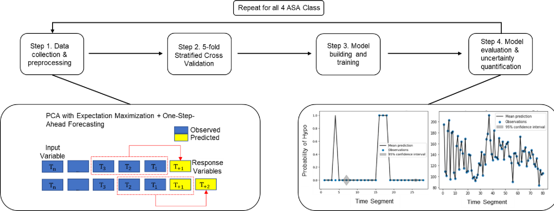
Step 1 collects data and preprocess data with time windows; Step 2 splits dataset into training and testing; Step 3 trains the model; Step 4 evaluates the model and summarizes the performance.

Table 1.

Characteristics of the cohort

Variable	Overall Population Set (n = 562)
Demographic
Age	48 (19, 90)
Female	562 (100%)
Comorbidity
Hypertension	248 (44.0%)
Congestive Heart Failure	14 (2.5%)
Valvular Disease	6 (1.1%)
Dysrhythmia	24 (4.3%)
Hypotension	3 (0.5%)
Coronary Artery Disease	15 (2.7%)
Dyslipidemia	84 (14.9%)
Peripheral Vascular Disease	2 (0.1%)
Syncope	1 (0.2%)
Abnormal EKG	12 (2.1%)
Emergency Surgery	3 (0.5%)
Preop Vitals
Temperature, Fahrenheit	98 (95.4, 99.7)
Systolic Blood Pressure, mm Hg	131.5 (81, 186)
Diastolic Blood Pressure, mm Hg	75 (39, 114)
Heart Rate, BPM	78 (42, 123)
Oxygen Saturation	99 (70, 100)
Respiratory Rate	17 (8, 25)

Note: Categorical variables represented as frequency (%). Continuous variables represented as median (25th percentile, 75th percentile), except age, which is median (minimum, maximum).

Classification Results

Figure 3 presents the results for binary prediction on hypotension for all four models. For ASA Class 1, BNNMR yielded the highest sensitivity of 1. For Classes 2 and 3, BNN had the highest sensitivity of 0.429 and 0.415, respectively. For Class 4, BNNMR and GP were tied with the highest sensitivity of 0.857. Even though BGLM achieves a single highest sensitivity of 0.889 within Class 4, it has poor performance on all other three classes compared to BNN and BNNMR. Overall, the BNNMR model produced two best sensitivities, while the regular BNN did on three. However, the highest sensitivity score of 1 by BNNMR for Class 1 is notable. Without clustering data into 4 datasets using ASA class caused all models suffer lower sensitivity score. (The detailed numerical results of each model can be found in Table S2 under the Supplementary materials.)

Figure 3. Classification performance for all models.

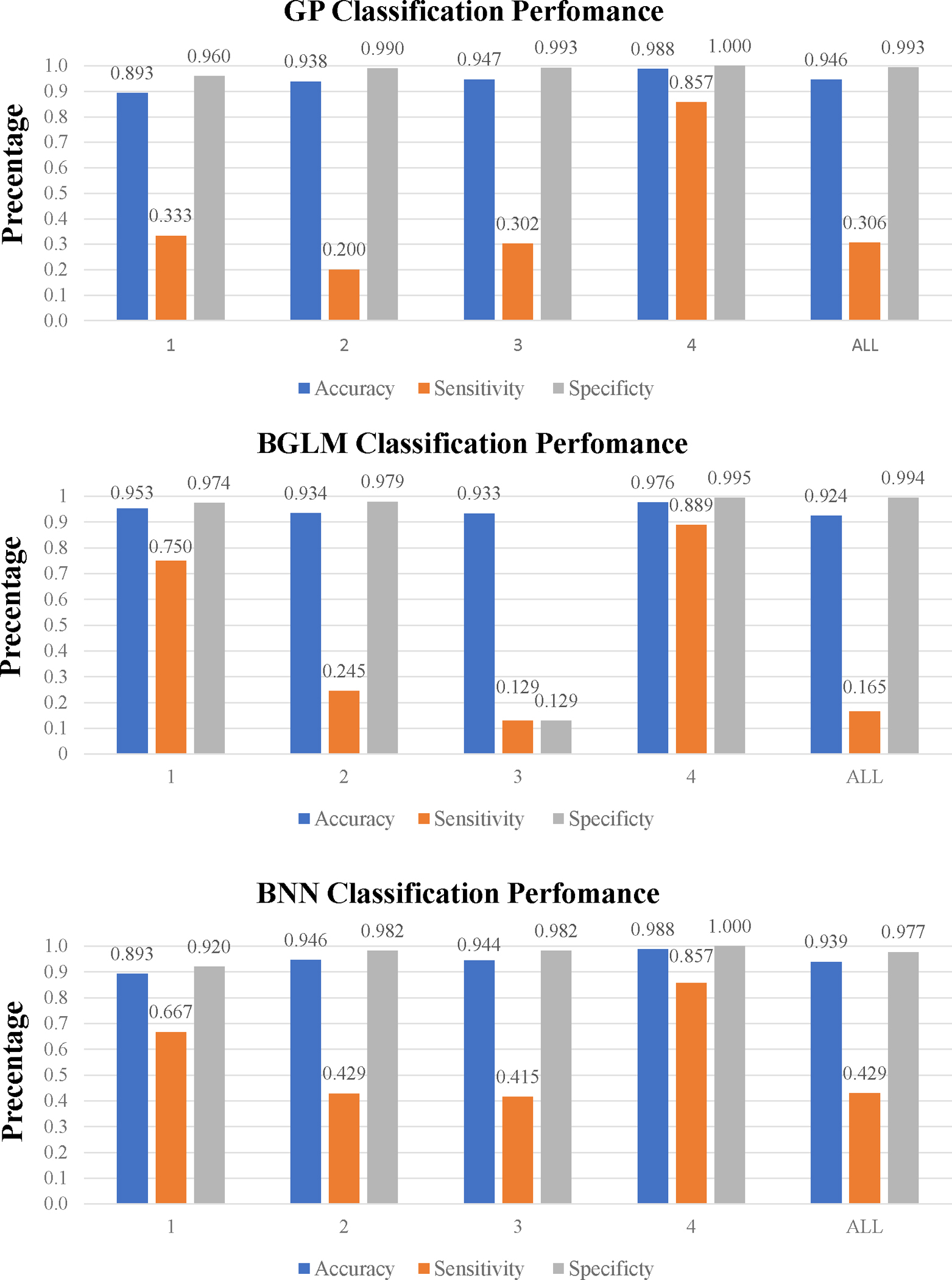
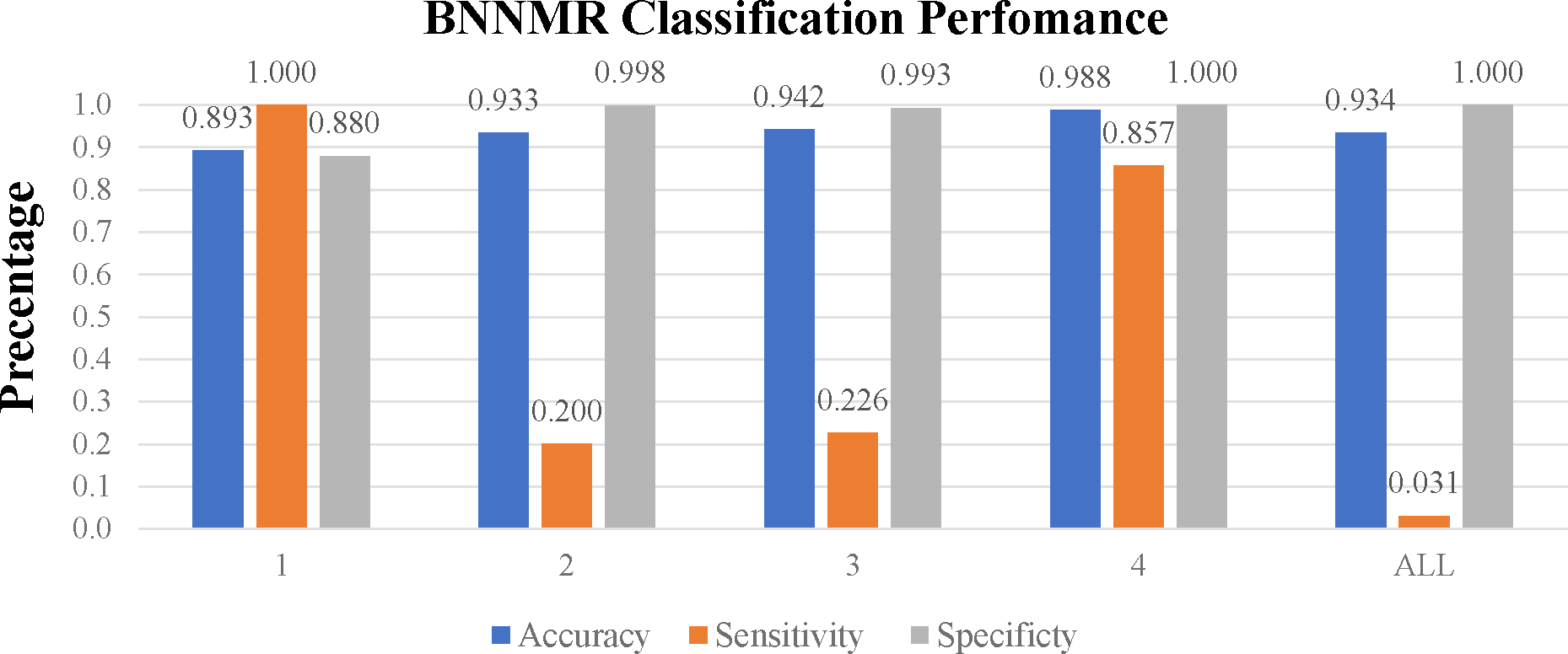
(Numerical tables in Table S2 under Supplementary Materials)

Regression Results

Table 2 displays the predicted mean systolic and diastolic blood pressures by the four models. GPR outperformed BNN and BNNMR models with RMSE ranging from 0.3 to 9.2 for predicting the systolic blood pressure, and from 0.8 to 6.6 for predicting the diastolic blood pressure across four ASA classes. However, without controlling the ASA class, GPR models yielded RMSE of 126.89 and 8.08 for predicting systolic and diastolic blood pressures, respectively. Between the two BNN models, BNNMR outperformed the regular BNN for three of the four ASA classes.

Table 2.

Regression Result Comparison

	RMSE
	ASA Class	Systolic	Diastolic
GPR	1	2.072	2.152
	2	7.539	6.573
	3	9.214	5.371
	4	0.295	0.831
	ALL	126.894	8.084
BGLM	1	2.175	3.651
	2	13.861	13.525
	3	17.560	11.513
	4	22.426	22066
	ALL	0.762	0.765
BNN	1	3.461	4.917
	2	13.861	11.001
	3	11.799	57.627
	4	3.019	3.242
	ALL	2.397	2.0563
BNNMR	1	3.029	2.705
	2	13.600	13.156
	3	16.654	11.531
	4	3.346	2.259
	ALL	16.925	12.379

Finally, Figure 4 depicts the 95% confidence interval (shaded in grey), as a measure of uncertainty quantification for ASA Class 4 (Other three similar figures for ASA Class 1–3 can be found in the online supplementary materials section). Collectively, these figures suggest that the GPR model yielded the narrowest thus the best 95% confidence intervals, for all ASA classes. In addition, the unexpected large RMSE (22066) from BRR model is obtained since the BGLM is not robust to outliers, hence producing large predictive uncertainty with biased prediction.

Figure 4. Uncertainty comparison among GPR, BNNR, BNNMR, and BGLM for ASA Class 4.

(Note: Black line represents the prediction of mean values; a blue dot represents the observed value from the test set; grey region represents the 95% confidence intervals)

Overall Evaluations

For classification, BNNMR has the best sensitivity in ASA Class 1 and ASA Class 4. For regression, Gaussian Process outperformed BNN and BNNMR with lower RMSE. GPR yielded the strongest uncertainty intervals for four ASA Classes. The benefit of dividing data into subsets based on ASA physical status class is confirmed. Table 3 shows the BNNMR algorithm model performances on each ASA class’s testing dataset when it was trained on the combinations of the initial ASA class training dataset and the individual dataset of the combined ASA class. Note that all diagonal elements represent the analysis without combining ASA classes. This analysis is executed by observing key metrics: the RMSE for regression models, specificity and sensitivity for classification models, and all three for mixed models. Table 3 reveals that the models’ performances are the best, in the diagonal blocks, i.e., when both the training and testing data are from the same ASA class. This trend is consistent across all ASA classes, indicating that the model generalizes best when exposed to similar data during both its training and testing. However, when the model is trained on one ASA class and tested on another, there is a noticeable disparity in performances. Take the pairs with ASA Class 4 as examples, all pairs have worse performance in both regression and classification when compared to the original BNNMR model trained on single ASA class data. For all other pairs, either the RMSE values tend to be higher, or the sensitivity shows significant variations. This suggests that each ASA class has unique characteristics that the model learns effectively when trained specifically on that ASA class. Combining data across ASA classes worsens the ML model prediction performance. In conclusion, this cross-class analysis suggests that ASA class has significant impact on model performance, and one should control this factor when developing ML models.

Table 3.

Results in BNNMR considering other ASA Class Scores

Training Dataset	ASA 1	ASA 1 & 2	ASA 1 & 3	ASA 1 & 4
		Testing Dataset ASA 1
RMSE (SBP)	3.029	2.92	2.911	2.918
RMSE (DBP)	2.705	2.381	2.368	2.408
Specificity	0.88	0.96	0.96	0.92
Sensitivity	1	0.667	0.333	0.667
Training Dataset	ASA 2 & 1	ASA 2	ASA 2 & 3	ASA 2 & 4
	Testing Dataset ASA 2
RMSE (SBP)	50.013	13.6	50.005	50.011
RMSE (DBP)	36.983	13.156	37.012	36.998
Specificity	0.832	0.998	0.832	0.832
Sensitivity	0.343	0.2	0.343	0.371
Training Dataset	ASA 3 & 1	ASA 3 & 2	ASA 3	ASA 3 & 4
	Testing Dataset ASA 3
RMSE (SBP)	49.153	49.208	16.654	49.156
RMSE (DBP)	35.196	35.216	11.531	35.184
Specificity	0.859	0.858	0.993	0.856
Sensitivity	0.472	0.472	0.226	0.472
Training Dataset	ASA 4 & 1	ASA 4 & 2	ASA 4 & 3	ASA 4
	Testing Dataset ASA 4
RMSE (SBP)	55.48	55.454	55.468	3.346
RMSE (DBP)	29.414	29.411	29.403	2.259
Specificity	0.767	0.767	0.767	1
Sensitivity	0	0	0	0.857

From a clinical viewpoint, the findings suggest that ASA 1 and ASA 4 patients have more pronounced or distinguishable patterns that can impact intraoperative hypotension predictions. Thus, the machine learning model can effectively identify hypotension risk in these groups. However, for intermediate classes (ASA 2 and ASA 3), the impact is less clear, and the model might not be as adept at making precise predictions.”

Discussions

Our study is distinct from existing literature in three ways. First, in order to provide trustable and usable predictions, we focus not only on mean values of the diastolic and systolic blood pressures, but more importantly their predictive uncertainty indicated by confidence levels (e.g., 95%), which is referred to as uncertainty quantification. This is extremely valuable to assist clinicians to make informed decisions [22], but largely lacking in anesthesiology literature. For example, a prediction with large uncertainty (e.g., hypotension probability of 0.6±0.3) can lead to reduced trust from clinicians as the machine learning model seems to be “hesitating” (i.e., not well trained) to make such prediction. Additionally, the uncertainty quantification directly acknowledges all prediction models have inherent uncertainty arising from various sources, such as model assumptions, data errors, and unobserved confounding factors [23]. Second, patients with different ASA physical status classifications have different physiological and pathophysiological responses to blood pressure change [24–26]. However, existing research on predicting blood pressures and hypotensive event [1–6, 27] mostly uses one predictive tool for all patients. Expectedly, the prediction performance varies significantly for a testing population with diverse baseline characteristics [28]. Therefore, we train distinct machine learning models using data subsets for each ASA physical status class. Third, we jointly predict two types of responses, i.e., the continuous systolic and diastolic pressures and the binary hypotensive event, for the same future time. By utilizing the association between blood pressures and hypotension, we expect the mixed response model to yield higher prediction accuracy and lower predictive uncertainty.

We found that BGLM, GP regression, BNN regression, and BNNMR can quantify uncertainty in blood pressure prediction, but only GP regression produced uncertainty intervals within reasonable range. All models have accurate predictions in ASA Class 1 and 4. BNNMR has overall the best classification prediction on hypotensive event, and its prediction is 100% accurate in ASA Class 1 among our collected data. The performances of all models in regression, as well as in classification, are similar for the less predictable ASA classes 3 and 4.

Overall, our computational results positively support four main methodological novelties. The first novelty is partitioning of the dataset based on patient’s ASA physical status classification. Our results demonstrated the performance gain in predicting blood pressures and hypotensive event by training different models for different ASA classes. When treating the ASA classes as a categorical variable, we created distinct groups of patients with four levels of risks based on their health status. This prevents the model from being biased by patients’ varying baseline characteristics. Our results showed that all four models produced significantly better performances when trained on data subsets for individual ASA classes, when compared to those trained on the entire dataset. Recently, a commercially available Hypotension Prediction Index by Edwards Lifesciences was found to perform no better than only using mean blood pressure to predict hypotension in 5 minutes [29]. This demonstrates the need for more accurate and perhaps more tailored machine learning models to predict blood pressures or hypotension for different patient populations. Recent studies have evaluated the commercially available Hypotension Prediction Index (HPI), an algorithm developed by Edwards Lifesciences from arterial pressure waveform characteristics, in predicting and managing hypotensive events. Li et al systematically reviewed the effectiveness of HPI in preventing intraoperative hypotension during noncardiac surgeries and found HPI-guided hemodynamic management could potentially surpass routine approaches, particularly for patients above 60 years old and those with higher ASA physical statuses [30]. Shin et al. found that HPI was helpful to predict hypotensive occurrences during cardiac surgeries requiring cardiopulmonary bypass [31]. Interestingly, a recent cross-correlation analysis was performed between the normalized HPI and mean arterial blood pressure (MAP) in 33 adult, high-risk noncardiac surgery patients found that HPI and MAP are highly correlated without time delay. Authors suggested that MAP 70–75mmHg may yield a prediction of intraoperative hypotension comparable to HPI [29].

HPI is developed from known physiological parameters (arterial waveforms), requiring relatively less data, offering high interpretability, demanding lower computational power, and making it apt for real-time clinical applications. In contrast, deep learning, embodied by neural networks, learns patterns from vast datasets without relying on predefined relationships. Their inherent flexibility allows them to be trained for various predictive tasks. Therefore, we aim to refine and expand our current research by encompassing a more diverse patient population, moving beyond the existing dataset of 562 female participants. Our finding suggest that ASA classifications significantly affect machine learning model’s performances and is consistent with the recently noticed limitations of HPI, which did not consider ASA classifications [29].

Our primary focus is to test the algorithm across a multitude of surgery types, such as cardiac procedures, to ascertain its generalizability. In contrast to the HPI, which primarily relies on arterial waveforms, our proposed model will incorporate a broader spectrum of factors, encompassing both preoperative and intraoperative variables. By harnessing the modern advantage of electronic anesthesia records, we plan to seamlessly integrate these data in the final clinical support system to reduce intraoperative hypotension. The goal is to develop a model that not only interfaces with the Electronic Medical Record (EMR) system but also elevates the accuracy in predicting blood pressure. This comprehensive approach seeks to harmonize machine-driven predictions with human medical expertise.

The second novelty is the uncertainty quantification of the prediction. Uncertainty quantification can help increase trust and confidence by providing information on the confidence level of the prediction, the range of possible outcomes, and the potential sources of error or bias in models. These are critically important towards trustworthy clinical decision-making for ML models [32]. Especially in medicine, decisions based on prediction models can lead to significant consequences for patient health and safety.

The third novelty is to jointly predict both binary and continuous response variables by quantifying the hidden association among these response variables. Compared to the regression (continuous) response, the binary response contains less information because of the data aggregation. The continuous response contains all the information from the binary response. The information and the hidden association among mixed responses are ignored if predictors and response variables for both types are used separately. By fully exploiting the information and relationships between both predictors and responses, the BNNMR can not only provide better predictions, but also quantify the hidden correlation among mixed responses [12]. For both ASA Class 1 and 4, BNNMR provided a more reasonable uncertainty intervals than BNN.

The fourth novelty is the combined use of the one-step forward sliding window technique and PCA to fill out missing values in medical records, a common issue when applying ML models to medical data. The combined method allowed us to maximize the use of available temporal data and led to satisfactory performance on predicting blood pressure and hypotensive event for ASA Class 1 and Class 4 patients. Existing literature on hypotension prediction methods either do not explicitly address missing values or simply impute with constant mean values [1–6, 27].

Based on our analysis of the study results, it was evident that models trained without controlling for ASA classes yielded both lower sensitivity and higher uncertainty. To address these shortcomings and improve the model’s performance in terms of sensitivity and quantification values, we have identified a potential solution: dividing the data based on ASA classes. By doing so, we anticipate that the model will be better equipped to discern patterns and make more accurate predictions specific to each class, thus resulting in enhanced performance metrics. Data augmentation expands the training dataset by creating modified versions of existing data, aiding in model generalization. To address class imbalance, the SMOTE technique generates synthetic samples in the feature space and enhances model performances [33]. However, since our methods jointly predict both classification and regression targets, no existing data augmentation algorithms can be applied in our cases. To understand the specific impact of each ASA class on intraoperative hypotension predictions, further research might focus on dissecting the unique characteristics of each class, especially the intermediate ones (ASA 2 and ASA 3). Understanding these specifics can provide more clarity on whether low or high ASA classes inherently have more impact.

There are several limitations to this study. First, the dataset is limited to the single center, retrospective, female only for hysterectomy patient population. It is not clear whether the research findings could be generalized to other patient groups. Second, we presented uncertainty quantification as 95% prediction intervals, but without specific threshold values that clinicians could directly apply towards treatment or intervention decisions. The last limitation is the reduced sample size resulting from partitioning the dataset based on the patient’s ASA physical status classification. Historically, collecting comprehensive datasets from paper records was challenging and error prone. However, with the healthcare industry’s shift towards electronic medical records (EMRs), data collection has become more efficient and accurate. This advancement will facilitate future research to 1) gather more data on patients’ ASA physical status classifications to increase our sample size, and 2) continually refine our analysis as new data becomes available, ensuring our findings remain relevant and precise.

Conclusions

The BNNMR and GP model were both found to produce high quality predictions of systolic and diastolic blood pressures for patients in all ASA Classes. While GP regression yielded lower prediction uncertainties, the BNNMR model provided a more accurate classification of hypotensive events. The use of a divided dataset based on ASA physical status class led to more accurate and interpretable performance of both GP and BNNMR models in predicting hypotensive events. This confirms the hypothesis that ASA physical status class affects machine learning models’ performances. Finally, this initial attempt of quantifying uncertainties associated with hypotension predictions produced expected and encouraging results that can potentially benefit clinical decision making. All these findings should be validated in a larger, multi-center dataset with diverse patients and surgical procedures.

Highlights.

• Developing distinct prediction models by controlling the ASA physical status class to improve sensitivity in predicting hypotensive event

• Quantifying uncertainty associated with prediction models

• Demonstrating the value and need for including uncertainty quantification in performance metrics for any prediction models in clinical research

• A novel Bayesian neural network with multivariate mixed responses to jointly predict the binary hypotension indicator and the continuous diastolic and systolic blood pressures

• A novel data imputation method of combining the one-step forward sliding window technique and principal component analysis to address block-wise missing data often seen in perioperative medical records

• Interdisciplinary research between medicine and industrial and systems engineering

Highlights.

• Developing distinct prediction models for each ASA physical status class

• Quantifying uncertainty associated with prediction

• Combining one-step forward sliding window and principal component analysis techniques for data imputation

References

- [1].Jeong Y-S, Kang AR, Jung W, Lee SJ, Lee S, Lee M, et al. Prediction of blood pressure after induction of anesthesia using deep learning: A feasibility study. Applied Sciences. 2019;9:5135. [Google Scholar]
- [2].Lee J, Woo J, Kang AR, Jeong Y-S, Jung W, Lee M, et al. Comparative analysis on machine learning and deep learning to predict post-induction hypotension. Sensors. 2020;20:4575. [DOI] [PMC free article] [PubMed] [Google Scholar]
- [3].Chen J-B, Wu K-C, Moi S-H, Chuang L-Y, Yang C-H. Deep learning for intradialytic hypotension prediction in hemodialysis patients. IEEE Access. 2020;8:82382–90. [Google Scholar]
- [4].Lee S, Lee H-C, Chu YS, Song SW, Ahn GJ, Lee H, et al. Deep learning models for the prediction of intraoperative hypotension. British journal of anaesthesia. 2021;126:808–17. [DOI] [PubMed] [Google Scholar]
- [5].Fritz BA, Cui Z, Zhang M, He Y, Chen Y, Kronzer A, et al. Deep-learning model for predicting 30-day postoperative mortality. British journal of anaesthesia. 2019;123:688–95. [DOI] [PMC free article] [PubMed] [Google Scholar]
- [6].Hofer IS, Lee C, Gabel E, Baldi P, Cannesson M. Development and validation of a deep neural network model to predict postoperative mortality, acute kidney injury, and reintubation using a single feature set. NPJ digital medicine. 2020;3:58. [DOI] [PMC free article] [PubMed] [Google Scholar]
- [7].An R, Pang Q-Y, Liu HL. Association of intra‐operative hypotension with acute kidney injury, myocardial injury and mortality in non‐cardiac surgery: A meta‐analysis. International journal of clinical practice. 2019;73:e13394. [DOI] [PubMed] [Google Scholar]
- [8].Yu Q, Qi J, Wang Y. Intraoperative hypotension and neurological outcomes. Current Opinion in Anesthesiology. 2020;33:646–50. [DOI] [PubMed] [Google Scholar]
- [9].Maheshwari K, Turan A, Mao G, Yang D, Niazi A, Agarwal D, et al. The association of hypotension during non‐cardiac surgery, before and after skin incision, with postoperative acute kidney injury: a retrospective cohort analysis. Anaesthesia. 2018;73:1223–8. [DOI] [PubMed] [Google Scholar]
- [10].Walsh M, Devereaux PJ, Garg AX, Kurz A, Turan A, Rodseth RN, et al. Relationship between intraoperative mean arterial pressure and clinical outcomes after noncardiac surgery: toward an empirical definition of hypotension. Anesthesiology. 2013;119:507–15. [DOI] [PubMed] [Google Scholar]
- [11].Gregory A, Stapelfeldt WH, Khanna AK, Smischney NJ, Boero IJ, Chen Q, et al. Intraoperative hypotension is associated with adverse clinical outcomes after noncardiac surgery. Anesthesia and analgesia. 2021;132:1654. [DOI] [PMC free article] [PubMed] [Google Scholar]
- [12].Kang X, Chen X, Jin R, Wu H, Deng X. Multivariate regression of mixed responses for evaluation of visualization designs. IISE Transactions. 2020;53:313–25. [Google Scholar]
- [13].Chen X, Lau N, Jin R. PRIME: A personalized recommender system for information visualization methods via extended matrix completion. ACM Transactions on Interactive Intelligent Systems. 2021;11:1–30. [Google Scholar]
- [14].Roweis S EM algorithms for PCA and SPCA. Advances in neural information processing systems. 1997;10. [Google Scholar]
- [15].Guo Y, Chen H. Fault diagnosis of VRF air-conditioning system based on improved Gaussian mixture model with PCA approach. International journal of refrigeration. 2020;118:1–11. [Google Scholar]
- [16].Chu C-SJ. Time series segmentation: A sliding window approach. Information Sciences. 1995;85:147–73. [Google Scholar]
- [17].Chou J-S, Nguyen T-K. Forward forecast of stock price using sliding-window metaheuristic-optimized machine-learning regression. IEEE Transactions on Industrial Informatics. 2018;14:3132–42. [Google Scholar]
- [18].Roehrig CS. Conditions for identification in nonparametric and parametric models. Econometrica: Journal of the Econometric Society. 1988:433–47. [Google Scholar]
- [19].Khan MS, Coulibaly P. Bayesian neural network for rainfall‐runoff modeling. Water Resources Research. 2006;42. [Google Scholar]
- [20].Le TD, Beuran R, Tan Y. Comparison of the most influential missing data imputation algorithms for healthcare. 2018 10th international conference on knowledge and systems engineering (KSE): IEEE; 2018. p. 247–51. [Google Scholar]
- [21].Gelfand AE. Gibbs sampling. Journal of the American statistical Association. 2000;95:1300–4. [Google Scholar]
- [22].Kappen T, Beattie WS. Perioperative hypotension 2021: a contrarian view. British Journal of Anaesthesia. 2021;127:167–70. [DOI] [PubMed] [Google Scholar]
- [23].Mathis MR, Kheterpal S, Najarian K. Artificial intelligence for anesthesia: what the practicing clinician needs to know: more than black magic for the art of the dark. Anesthesiology. 2018;129:619–22. [DOI] [PMC free article] [PubMed] [Google Scholar]
- [24].MacKay DJ. Bayesian neural networks and density networks. Nuclear Instruments and Methods in Physics Research Section A: Accelerators, Spectrometers, Detectors and Associated Equipment. 1995;354:73–80. [Google Scholar]
- [25].Schulz E, Speekenbrink M, Krause A. A tutorial on Gaussian process regression: Modelling, exploring, and exploiting functions. Journal of Mathematical Psychology. 2018;85:1–16. [Google Scholar]
- [26].Nelder JA, Wedderburn RW. Generalized linear models. Journal of the Royal Statistical Society Series A: Statistics in Society. 1972;135:370–84. [Google Scholar]
- [27].Kendale S, Kulkarni P, Rosenberg AD, Wang J. Supervised machine-learning predictive analytics for prediction of postinduction hypotension. Anesthesiology. 2018;129:675–88. [DOI] [PubMed] [Google Scholar]
- [28].Sessler DI, Khan MZ, Maheshwari K, Liu L, Adegboye J, Saugel B, et al. Blood pressure management by anesthesia professionals: evaluating clinician skill from electronic medical records. Anesthesia & Analgesia. 2021;132:946–56. [DOI] [PubMed] [Google Scholar]
- [29].Mulder MP, Harmannij-Markusse M, Donker DW, Fresiello L, Potters J-W. Is Continuous Intraoperative Monitoring of Mean Arterial Pressure as Good as the Hypotension Prediction Index Algorithm? Anesthesiology. 2023;138:657–8. [DOI] [PubMed] [Google Scholar]
- [30].Li W, Hu Z, Yuan Y, Liu J, Li K. Effect of hypotension prediction index in the prevention of intraoperative hypotension during noncardiac surgery: a systematic review. Journal of Clinical Anesthesia. 2022;83:110981. [DOI] [PubMed] [Google Scholar]
- [31].Shin B, Maler SA, Reddy K, Fleming NW. Use of the hypotension prediction index during cardiac surgery. Journal of cardiothoracic and vascular anesthesia. 2021;35:1769–75. [DOI] [PubMed] [Google Scholar]
- [32].Chen X, Kang X, Jin R, Deng X. Bayesian Sparse Regression for Mixed Multi-Responses with Application to Runtime Metrics Prediction in Fog Manufacturing. Technometrics. 2023;65:206–19. [Google Scholar]
- [33].Wong SC, Gatt A, Stamatescu V, McDonnell MD. Understanding data augmentation for classification: when to warp? 2016 international conference on digital image computing: techniques and applications (DICTA): IEEE; 2016. p. 1–6. [Google Scholar]
Associated Data
This section collects any data citations, data availability statements, or supplementary materials included in this article.