The Impact of AI-Based Modeling on the Accuracy of Protein Assembly Prediction: Insights from CASP15

Abstract

In CASP15, 87 predictors submitted around 11,000 models on 41 assembly targets. The community demonstrated exceptional performance in overall fold and interface contact prediction, achieving an impressive success rate of 90% (compared to 31% in CASP14). This remarkable accomplishment is largely due to the incorporation of DeepMind’s AF2-Multimer approach into custom-built prediction pipelines. To evaluate the added value of participating methods, we compared the community models to the baseline AF2-Multimer predictor. In over 1/3 of cases the community models were superior to the baseline predictor. The main reasons for this improved performance were the use of custom-built multiple sequence alignments, optimized AF2-Multimer sampling, and the manual assembly of AF2-Multimer-built subcomplexes. The best three groups, in order, are Zheng, Venclovas and Wallner. Zheng and Venclovas reached a 73.2% success rate over all (41) cases, while Wallner attained 69.4% success rate over 36 cases. Nonetheless, challenges remain in predicting structures with weak evolutionary signals, such as nanobody-antigen, antibody-antigen, and viral complexes. Expectedly, modeling large complexes remains also challenging due to their high memory compute demands.

In addition to the assembly category, we assessed the accuracy of modeling interdomain interfaces in the tertiary structure prediction targets. Models on seven targets featuring 17 unique interfaces were analyzed. Best predictors achieved a 76.5% success rate, with the UM-TBM group being the leader. In the interdomain category, we observed that the predictors faced challenges, as in the case of the assembly category, when the evolutionary signal for a given domain pair was weak or the structure was large. Overall, CASP15 witnessed unprecedented improvement in interface modeling, reflecting the AI revolution seen in CASP14.

INTRODUCTION

The understanding of protein interactions at the atomistic scale is crucial for studying cellular function. Experimental techniques like X-ray diffraction, NMR spectroscopy, and cryo-electron microscopy (cryo-EM) provide high-resolution structures of protein complexes¹. However, in cases where experimental approaches face limitations, modeling becomes valuable^2–5. In particular, homology modeling is employed when there is a resolved structure of an evolutionarily related complex, while docking is preferred in the absence of such a template. Various strategies, including coevolution integration and the use of available experimental data, have been implemented to enhance docking accuracy^6–12. For intricate cases involving intertwined complexes, fold-and-dock strategies are employed^13,14.

The CAPRI blind docking competition has been evaluating the state-of-the-art in assembly modeling since 2002^15,16. In 2014, CAPRI joined forces with CASP to assess the prediction of protein complexes on a larger scale. Several rounds of CASP-CAPRI experiments have been conducted, shedding light on the capabilities and limitations of assembly modeling approaches^15,17–23. A major limitation in protein complex modeling has been the absence of reliable templates for modeling the monomer structures of an assembly^20,24. This limitation has been alleviated to a large extent with the release of AlphaFold2 (AF2), an artificial intelligence (AI) tool that has made unprecedented progress in tertiary structure prediction²⁵. In CASP14, AF2 demonstrated high accuracy in modeling tertiary structure targets regardless of the prediction difficulty^25,26. Consequently, the release of AF2 Protein Structure Database in 2022, with over 214 million predicted protein structures covering nearly all UniProt sequences, has significantly impacted the field of structural biology^27,28.

Since the release of AF2, scientists have sought to incorporate this framework into their modeling pipelines. The simplest way to employ tertiary structure modeling methods to quaternary structure modeling was to join individual sequences of complex subunits into a longer, artificial sequence by means of adding an artificial glycine linker between monomers or introducing a sequence gap between multiple chains^29–32. These approaches showed improvement over classical docking methodologies^33–35. In 2021, DeepMind released AlphaFold-Multimer (AF2M, version 2.2), the multimeric version of AF2 specifically retrained on biological interfaces³². AF2M outperformed previously outlined AF2-monomer modifications in the case of heteromers. Although DeepMind did not participate in CASP15, they did so indirectly since the vast majority of assembly groups adopted AF2M in their modeling pipelines³⁶.

In CASP15, to enhance the model accuracy, most of the groups experimented either with the multiple sequence alignment (MSA) input or with the AF2M sampling parameters. Among these, many benefitted from feeding their improved custom MSA into AF2M. A few utilized increasing the number of recycles (how many times the solutions are fed back to the AI-model), generating more models by starting from different random seeds or activating the dropout layers in the network. While tracing the specific AF2M modification strategies utilized by the community, we analyzed 41 assembly targets, considering the capabilities and limitations of the presented AF2M modifications. Our analysis shows where the community could push the boundaries of AI-based assembly modeling forward. It also highlights the remaining open challenges in the field.

METHODS

Assembly Assessment: General Concepts

Predictors in the CASP15 assembly category were provided with the stoichiometry information. We verified the symmetries of the targets in collaboration with the CAPRI team by using AnAnaS³⁷ and biological assemblies by using EPPIC³⁸ and PISA^39,40. Additionally, we assessed the interface properties, where needed by using PISA. Four targets, T119o, T1176o, T1176ov1, and T1184o, were canceled due to mismatch between the biological interfaces assigned by us and by the authors (Figure S1A). Targets H1171 and H1172 were multiple-conformation complexes spanning 1.5Å all-atom RMSD range. While assessing H1171 and H1172, we compared submitted models to all available conformers (two for H1171 and four for H1172) and reported the results for the top-scoring model of each group.

Targets were classified into three prediction difficulty categories: easy if there is a structural template for the entire assembly, medium if there is a partial template for subunits or their interactions, and hard if there is no template. HHPred (https://toolkit.tuebingen.mpg.de/tools/hhpred)^41,42 was used for template search. Additionally, we grouped targets based on their complex types, including homomeric (consisting of identical subunits), heteromeric (formed by different subunits), intertwined (with small segments or domains exchanged between subunits), nanobody-antigen, and antibody-antigen.

Evaluation unit definitions

Evaluation of assembly targets requires establishing a structural correspondence between the constituent chains of the model and experimental structures. This proved to be a challenging and time-consuming task for complexes with many subunits. Recently, Gabriel Studer suggested a greedy heuristic approach (https://git.scicore.unibas.ch/schwede/casp15_ema) to solve the chain mapping problem⁴³. This development allowed us to proceed with the evaluation of large complexes directly, without splitting them in subcomplexes as we did in CASP14²⁰. However, we still needed to alter four targets.

• H1114 is an A4B8C8 bacterial assembly with C4 symmetry. In this complex, monomer A is forming an intertwined tetrameric tube, which interacts with monomer B. The prediction challenge in this complex was to form the intertwined tube and its interactions. To specifically focus on these interactions, we evaluated A4B2 assembly as a separate target H1114v2 (Figure S1B).

• H1166, H1167, H1168 are A1B1C1 immune complexes consisting of two antibody subunits (heavy and light chains) and an antigen molecule. To focus on the antibody-antigen interactions, we merged two antibody chains into a single chain, and formally assessed the complexes as hetero-dimers H1166v1, H1167v1, H1168v1 (Figure S1C).

Scoring and ranking

Submitted models were scored according to four metrics: two evaluates the accuracy of predicted interfaces—interface contact score (ICS, calculated as F1 score)¹⁸ and Interface Patch Score (IPS, calculated as Jaccard coefficient)¹⁸, and the other two evaluates overall fold - template modeling (TM) score⁴⁴, and local distance difference test (lDDT) score⁴⁵.

ICS measures the relationship between precision (P) and recall (R) of predicted inter-chain contacts. P is the fraction of the correct inter-chain contacts among all model inter-chain contacts. R is the fraction of correctly reproduced native inter-chain contacts. M and T represent model and target. Two residues are considered in contact when at least two of their non-hydrogen atoms (one from each residue) are within 5Å from each other.

$$ICS(M,T)=F1(P,R)=2\frac{P(M,T)\times R(M,T)}{P(M,T)+R(M,T)}$$ (Eq.1)

IPS is calculated as a Jaccard coefficient (J_c) over the interface amino acids (I) predicted by the model (I_M) compared to the target (I_T):

$$IPS(M,T)=J_C(M,T)=\frac{\left|I_M\cap I_T\right|}{\left|I_M\cup I_T\right|}$$ (Eq.2)

TM score measures the topological similarity of the model with respect to the target, where L and L_ali represent the target’s length and the number of equivalent residues in two structures, respectively. d_i is the distance between the i^th pair of equivalent residues in the two structures. The score is normalized by the scaling factor d₀.

$$\mathit{\text{TMscore}}=\frac{1}{L}\left[\sum _{i=1}^{L_{ali}}\frac{1}{1+d_i^2/d_0^2}\right]$$ (Eq.3)

IDDT measures the difference in the interatomic distances between a model and the target. It is calculated by examining distances between pairs of atoms in the target that fall within a predefined threshold. If the difference in these distances is within a threshold (15 Å), the interaction is considered preserved in the prediction. The final score is determined by averaging the fraction of accurately modeled interactions.

We consider a model successful if it scored above 0.50 on all metrics. Focusing our analysis on the regions where complex subunits interact, we define three interface prediction accuracy zones: poor (ICS < 0.50), good (0.50 ≤ ICS < 0.75) and high (ICS ≥ 0.75). To investigate the interface prediction improvement across different CASP rounds, we carried out a comparative distribution analysis. For this, we collected the best ICS values generated for a given difficulty class during every round. The distributions of these values were then represented with box-and-whisker plots.

Participants were ranked based on their relative performance according to all four evaluation metrics. A per-metric relative performance was calculated in terms of Z-scores reporting the number of standard deviations a particular model’s score is above or below the per-target population mean:

$$\text{Z-score}=(\text{score}-\text{mean})/\text{standard\_deviation}$$ (Eq.4)

Z-scores were calculated for two different model sets: all submitted models or models designated as model_1 (i.e., top-ranking models according to the predictor). Initially, Z-scores were computed on full model sets. Then outliers (models with Z-scores < −2) were removed, and Z-scores were re-calculated on the remaining models. Negative Z-scores were reset to 0 to avoid strong penalization of groups who underperformed. The final ranking score of a group was computed as a sum of combined per-metric Z-scores over all predicted targets:

$$\mathit{\text{CASP15 ranking score}}={\sum }_{\mathit{\text{targets}}}\frac{[\mathit{\text{Z-score}}(ICS)+\mathit{\text{Z-score}}(IPS)+\mathit{\text{Z-score}}(\mathit{\text{lDDT}})+\mathit{\text{Z-score}}(TM)]}{4}$$ (Eq.5)

Ranking on first models is considered for the ‘official’ CASP ranking.

The robustness of ranking is verified by the jackknife resampling. For this, initially, one target was excluded from the analysis, and the sum of Z-scores was calculated over the remaining targets. This process was repeated iteratively, excluding a different target at each step, until all targets were excluded for once. For the final ranking, we utilized the mean scores obtained from the jackknifing protocol. The standard deviations from the jackknifed data set are used as a measure of the results’ variability.

Naïve (baseline predictor)

Vast majority of CASP15 groups used the AF2M method as a starting point for their modeling. To help predictors in obtaining starting models, CASP organizers made an arrangement with Claudio Mirabello from the Elofsson group to run the public AF2M (version 2.2) method on all CASP15 targets and to submit their models to CASP as the NBIS-AF2-Multimer group (NBIS-AF2M). In our evaluation, these predictions were used as the baseline models. Hereafter, NBIS-AF2M will be referred to as the baseline or naive AF2M⁴⁶. We used the naive AF2M MSAs (deposited in http://duffman.it.liu.se/casp15/)⁴⁷ to calculate the depth of sequence profiles. By default, the input MSAs were generated by JackHMMER v3.3⁴⁸.The informational content of an MSA was evaluated with Neff, the number of effective sequences⁴⁹. Neff was calculated as

$$\mathit{\text{Neff}}=\sum _{i=1}^N\frac{1}{{\mathit{\text{ weight }}}_i}$$ (Eq.6)

where N is the number of sequences in the MSA. For each sequence i, weight_i is the sum of weight_ij over all the sequences in the MSA, while weight_ij is the sequence identity between any homologues sequence i and j in the MSA. The minimum sequence identity between i and j was set to 80% identical residues.

For the targets with subunits, we calculated the multimeric Neff as

$${\mathit{\text{Neff}}}_{\mathit{\text{multimeric}}}={\left({\mathit{\text{Neff}}}_1*\dots *{\mathit{\text{Neff}}}_N\right)}^{1/N},$$ (Eq.7)

where N is the number of different subunits.

The baseline AF2M method was run with default parameters (no_recycles=3, no_seeds=5)⁴⁶, except for T1173, T1174, and T1181, where the NBIS team set the number of recycles to 25. Models for large targets - H1111, H1114, H1115, H1135, H1137 - were built by MolPC⁵⁰. The final ranking was performed according to the model confidence score (0.8 · ipTM + 0.2 · pTM)³², where pTM is the predicted TM and ipTM is the same metric calculated over the interface.

To quantify the difference between the community performance and the baseline, we introduced a ΔICS score (Eq. 8). For each target, this score measures a gain in the ICS of the best community model over the AF2M one:

$$\Delta \text{ICS}={\text{ICS}}_{\text{best ICS scoring model}}-{\text{ICS}}_{\text{best ICS scoring naive model}}$$ (Eq.8)

If needed, buried surface area (BSA) and noncovalent intermonomer interactions were calculated with the COCOMAPS tool (https://www.molnac.unisa.it/BioTools/cocomaps/)⁵¹.

Interdomain Assessment: General Concepts

All multi-domain targets were considered as candidates for the interdomain assessment. If a tertiary structure target had multiple interfaces, each of them was considered as a potential interdomain target¹⁸. Domain pairs with weak interfaces were disregarded, and only interfaces with ten or more interacting residue pairs were considered. For the evaluation of interdomain interactions, we employed two interface metrics used in the assembly assessment: ICS and IPS, and, additionally, the global quaternary structure (QSglobal) score^52,53. The predictors were ranked according to the cumulative Z-score function:

$$\mathit{\text{CASP}}15\mathit{\text{ interdomain score}}={\sum }_{\mathit{\text{targets}}}\frac{\left[\mathit{\text{Z-score}}(ICS)+\mathit{\text{Z-score}}(IPS)+\mathit{\text{Z-score}}\left(Q{S}_{\mathit{\text{global}}}\right)\right]}{3}$$ (Eq.9)

Z-scores for each metric were calculated on the first models using the same procedure as explained above.

Visualization software

All plots in this paper were generated by using Python 3.8.10 with numpy, seaborn, matplotlib, pandas, and statistics libraries^54–58.

The structure figures were generated with PyMOL(TM) 2.5.2⁵⁹.

RESULTS AND DISCUSSION

General Overview of the CASP15 Assembly Prediction Category

In CASP15, 40 protein complexes were offered as prediction targets (Table 1, Figure S2). twenty-nine of them were solved by X-ray crystallography, and the remaining 11 by cryo-EM. Half of the structures exhibited various degrees of cyclic symmetries. The target complexes contained from 2 to 27 subunits, with dimers prevailing. The homomeric cases comprised half of the assembly targets, including ten intertwined assemblies. The heteromeric cases consisted of three intertwined complexes (H1114, H1114v2 and H1137), one host-pathogen complex (H1129), and eight immunity complexes - five nanobody-antigen (H1140-H1144) and three antibody-antigen (H1166-H1168). The nanobody-antigen series involved the binding of five different nanobodies to the catalytic domain of mouse CNPase, an enzyme responsible for regulating cyclic nucleotide synthesis⁷⁰. While sharing a moderate sequence identity (ranging between 62%−73%), the nanobodies adopt distinct conformations (ranging between 3–7 Å all-atom RMSD) when bound to their targets. In the case of antibody-antigen series, the N-terminal domain of the SARS-CoV2 nucleocapsid protein was bound to different human antibodies, derived from COVID-19-infected individuals. The antibodies’ light and heavy chains exhibited moderate to high sequence identity, ranging from 43% to 81% and 74% to 96%, respectively, leading to 4–6 Å all-atom RMSD variations. In addition to these cross-species and immunity complexes, the primary target sources were bacterial and eukaryotic cells. Five targets presented different conformational states that were induced by ligand binding, mutation, or buffer conditions. The heptameric (H1171) and octameric (H1172) Holliday junction targets showcase the ligand-binding-induced conformational changes happening in their corresponding hexameric apo structure T1170o. Target T1109o, an isocyanide hydratase mutant, is an example of conformational changes due to a one-point mutation (D183→A183) in the wild-type structure T1110o. The point mutation resulted in an all-atom RMSD change of 11.2 Å. The ancient protein reconstruction target T1160o exhibits conformational differences compared to what is available in the literature due to different compounds used in the crystallization buffer⁷¹. T1161o is a mutation-induced version of T1160o, designed to explore the connection between an ancient DPBB (DNA/RNA polymerase binding) protein and a RIFT (ribosomal) protein. Each monomer of this protein had five amino acid differences compared to the original sequence, leading to a 1.6 Å all-atom RMSD change.

Table 1.

The CASP15 assembly targets with target’s pdb ids (if available), size, stoichiometry, symmetry, prediction difficulty, assembly class, taxonomy information, together with the experimental technique used to resolve them, as well as the group names who generated the best ICS model’s group. The targets shared with CAPRI are indicated with *.

Target ID	PDB ID	# of amino acids	Stoichiometry	Symmetry	Difficulty	Assembly classification	Taxonomy	Exp. Tech.	The best ICS model’s group
H1106*	7qih60	182	A1B1	-	Easy	Heteromer	Bacteria	X-Ray	OpenFold
H1111	-	4499	A9B9C9	C9	Medium	Heteromer	Bacteria	X-Ray	Yang-Multimer
H1114	7uus61	7360	A4B8C8	C4	Medium	Intertwined	Bacteria	EM	Yang
H1114v2	7uus61	1324	A4B2	-	Medium	Intertwined	Bacteria-Phage	EM	Venclovas
H1129*	8a8c62	1259	A1B1	-	Medium	Heteromer	Bacteria	EM	Wallner
H1134*	7ubz63	506	A1B1	-	Medium	Heteromer	Bacteria	X-Ray	Wallner
H1135*	-	1821	A9B3	C3	Medium	Heteromer	Eukaryotes	X-Ray	UltraFold
H1137*	8fef64	3343	A1B1C1D1 E1F1G2H1I1	-	Medium	Intertwined	Bacteria	EM	bio3d
H1140*	-	328	A1B1	-	Medium	Nanobody-antigen	Eukaryotes	X-Ray	Wallner
H1141*	-	329	A1B1	-	Medium	Nanobody-antigen	Nanobody-mouse	X-Ray	Zheng
H1142*	-	335	A1B1	-	Medium	Nanobody-antigen	Nanobody-mouse	X-Ray	Kiharalab
H1143*	-	329	A1B1	-	Medium	Nanobody-antigen	Nanobody-mouse	X-Ray	NBIS-AF2-multimer
H1144*	-	324	A1B1	-	Medium	Nanobody-antigen	Nanobody-mouse	X-Ray	Zheng
H1151*	-	539	A1B1	-	Easy	Heteromer	Bacteria	X-Ray	Wallner
H1157*	-	1446	A1B1	-	Medium	Heteromer	Eukaryotes	EM	Manifold-E
H1166v1*	-	553	A1B1 (H+L=1chain)	-	Medium	Antibody-antigen	Human-virus	X-Ray	Manifold-E
H1167v1*	-	540	A1B1 (H+L=1chain)	-	Medium	Antibody-antigen	Human-virus	X-Ray	ShanghaiTech
H1168v1*	-	564	A1B1 (H+L=1chain)	-	Medium	Antibody-antigen	Human-virus	X-Ray	DFolding-refine
H1171*	7pbl65	1918	A6B1	-	Easy	Heteromer, Ligand-induced change	Bacteria	EM	MultiFOLD
H1172*	7pbp65	1964	A6B2	-	Easy	Heteromer, Ligand-induced change	Bacteria	EM	Manifold-LC-E
H1185	-	928	A1B1C1D1	-	Easy	Heteromer	Eukaryotes	EM	Yang
T1109o*	-	442	A2	C2	Easy	Homomer, Mutation-induced change	Bacteria	X-Ray	Wallner
T1110o*	-	442	A2	C2	Easy	Intertwined	Bacteria	X-Ray	ColabFold
T1113o*	-	336	A2	C2	Hard	Intertwined	Bacteria	X-Ray	Manifold
T1115o*	-	3968	A16	C16	Medium	Homomer	Eukaryotes	EM	Venclovas
T1121o*	7til66	739	A2	C2	Medium	Intertwined	Bacteria	EM	DFolding-server
T1123o*	7uzt67	428	A2	C2	Medium	Homomer	Virus	X-Ray	MULTICOM_deep
T1124o	7ux868	738	A2	C2	Easy	Intertwined	Bacteria	X-Ray	MULTICOM
T1127o*	-	411	A2	C2	Easy	Intertwined	Plant	X-Ray	NBIS-AF2-multimer
T1132o*	-	603	A6	D3	Medium	Homomer	Bacteria	X-Ray	BAKER
T1153o*	-	530	A2	C2	Medium	Homomer	Eukaryotes	X-Ray	MULTICOM_qa
T1160o*	-	58	A2	C2	Easy	Intertwined, Condition-induced change	Ancient reconstruction	X-Ray	PEZYFoldings
T1161o*	-	96	A2	C2	Easy	Intertwined, Ancient reconstruction, mutation-induced	Ancient reconstruction	X-Ray	Wallner
T1170o*	7pbr65	1870	A6	C6	Easy	Homomer	Bacteria	EM	Yang
T1173o*	-	612	A3	C3	Hard	Intertwined	Bacteria	X-Ray	Yang
T1174o*	-	1014	A3	C3	Hard	Intertwined	Bacteria	X-Ray	Manifold-E
T1178o*	-	537	A2	-	Easy	Homomer	Virus	X-Ray	DFolding-server
T1179o*	-	505	A2	-	Easy	Homomer	Virus	X-Ray	DFolding
T1181o*	-	2064	A3	C3	Easy	Intertwined	Virus	X-Ray	PEZYFoldings
T1187o*	8ad269	330	A2	C2	Hard	Homomer	Plant	X-Ray	Venclovas
T1192o*	-	1246	A10	C10	Easy	Homomer	Eukaryotes	EM	Yang

All targets were evaluated with all interfaces contributing to the assessment score. For one of the targets with complicated stoichiometry (H1114, A4B8C8), the prediction challenge was to predict the smallest interface of the complex, formed between an intertwined tube and a protein dimer. We, therefore, additionally evaluated this subcomplex (A4B2) as a separate target (H1114v2) (Figure S1B). This increased the total number of evaluated cases to 41. From the perspective of prediction difficulty, the targets were categorized into 16 easy, 21 medium, and four hard cases according to the principles outlined in Methods (see Table S1). Further details on the assembly targets are presented in Table 1, together with their structural depictions in Figure S2.

A record number of participants - 61 human and 26 server groups - took part in CASP15. These groups submitted a total of 11,000 models, presenting a load four times larger than that in the previous CASP (Table 2). All targets were shared with CAPRI, and most of them were selected for CAPRI prediction (Table 2). Among the 87 CASP15 participating groups, 60 submitted predictions on more than half of the targets. According to the CASP15 Abstract Book, 90% of the groups used the AF2M methodology in one way or another^36,46. Some groups directly used the standard setup of AF2M, while others tried to enhance the sampling and/or scoring procedures of AF2M by supplying custom MSAs, templates, increasing the number of recycles used in sampling, or activating the dropout layers in the AI model to increase sampling diversification. Only very few groups performed classical docking and template-based modeling, starting from the AF2 tertiary structure models. A small set of groups utilized normal mode analysis and short molecular dynamics to model conformational changes happening upon binding. A brief description of these methods can be found in the CASP15 Abstract Book⁴⁶. Finally, it is worth mentioning that all AF2M-dependent CASP groups encountered a bottleneck in the straight-on modeling of large complexes, which had to be modeled upon dissecting the whole assembly into smaller subcomplexes.

Table 2.

Statistics of CASP assembly rounds over the years, including the share of heteromeric targets, the number of targets having more than two chains, difficulty class shares, number of targets shared with the joint CAPRI round, maximum ICS profiles acquired for the hard targets, number of competitors and total number of models submitted, the top performing approaches.

CASP Round	No. of targets (heteromers/all)	No. of target more than two chains	Difficulty (easy/medium/hard)	No. of shared targets with CAPRI	Maximum ICS observed for hard targets	No. of groups/No. of models	Notable approaches
CASP12	8/30	14	9/6/15	15	0.15	108/1600	Homology modeling
CASP13	12/42	17	12/17/13	20	0.52	45/5000	Homology modeling
CASP14	17/22	13	2/20/6	12	0.48	39/2500	Homology modeling Docking DL-based contacts Fold-and-dock
CASP15	20/40	17	14/22/4	36	0.95	87/11,000	Mainly AF2-M based modeling

CASP15 witnessed an unprecedented improvement in assembly modeling

In CASP15, we employed four different metrics to evaluate the accuracy of assembly models (see Methods). Distributions of the evaluation scores for all targets are shown in Figure 1. As defined in Methods, we consider a model to be successful (or acceptable) if it scores above 0.50 according to all evaluation metrics. Strikingly, the CASP15 community could submit at least one successful model for 90% (37 out of 41) targets (Table 1). For comparison, only 31% of CASP14 targets had successful models. In CASP15, the failing targets correspond to two antibody-antigen complexes (H1166, H1167), one nanobody-antigen complex (H1142), and a viral homodimer (T1123o).

Figure 1. Per-target distributions of A. ICS, B. TM, C. IPS, and D. lDDT metrics calculated over the submitted models.

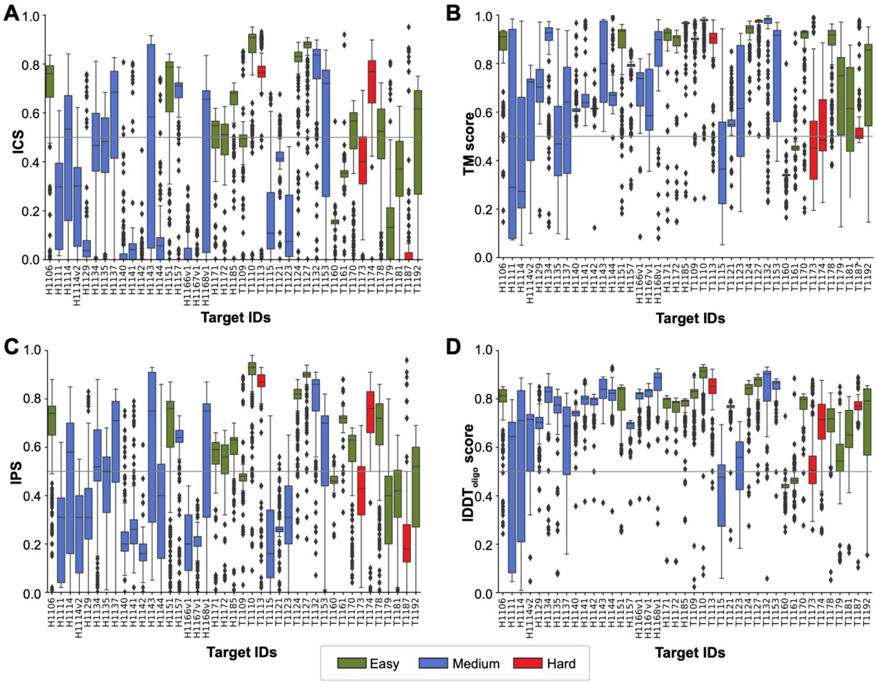
The box coloring follows the target difficulty color code (green: easy, blue: medium, red: difficult). The threshold for a model to be successful (0.50) is marked with a horizontal gray line.

Best predictors managed to model the overall fold of CASP15 targets extremely well. According to the fold similarity measures (lDDT and TM), 100% of CASP15 targets had models scoring over 0.50 (76% in CASP14) and 90% scoring over 0.75 (14% in CASP14). Getting interface regions accurately proved to be a slightly more difficult task, with 90% of CASP15 targets having models scoring over 0.50 according to the interface-based metrics IPS and ICS (31% in CASP14). Figure 2A confirms the striking improvement in the accuracy of interface modeling in the latest CASP. While in the pre-CASP15 editions the vast majority of targets (around 70%, red) were falling in the poor accuracy zone and only very small fraction (around 10%, green) in the high accuracy zone, in CASP15 the situation flipped with only less than 10% of targets being modeled poorly and more than a half modeled with high accuracy. The mean ICS score of the top models doubled from 0.37 in CASP14 to 0.74 in CASP15, almost reaching the lower boundary of the high-accuracy prediction zone (0.75 - see Methods for zone definitions). Notably, best models for some of the hardest targets almost perfectly reproduced native interfaces in CASP15 (e.g., ICS of 0.95 for T1187o or 0.90 for T1174o), while never crossing the 0.52 level in all previous CASP rounds (Table 2).

Figure 2.

A. Percentage of the best models in CASP12–15 falling into three interface accuracy bins: poor: ICS<0.50, red; good: 0.50 ≤ ICS < 0.75, blue; and high: ICS ≥ 0.75, green. B. Box-and-whisker plots for the best ICS scores generated in each round. The distributions are presented under different difficulty categories.

In CASP15, half of our targets were homomers. Also, the majority of the targets had complete or partial templates, de-facto making these targets easier for modeling. To ensure that the advancement observed in CASP15 was not solely due to the decreased difficulty of the target set, we conducted a difficulty-tuned comparative analysis of results across different CASP rounds (Figure 2B, Methods). This analysis demonstrated a significant performance enhancement across all difficulty categories, with an upward shift of 0.2 best-ICS for the easiest targets and 0.5 for the hardest ones, which shows that target difficulty was not the major determinant in the unprecedented accuracy improvement in CASP15.

Best performing CASP15 groups and their modeling strategies

We ranked participating groups according to a Z-score-based function composed of equally weighted inputs from ICS, IPS, lDDT, and TM metrics (Eq.5, Methods, Table S2). Zheng group ranked at the top (Figure 3A), followed by the second tier of groups including Venclovas and Wallner groups, and the third tier comprising Yang and Yang-Multimer. The robustness of the ranking is confirmed by the jackknife cross-validation. If we rank groups on the best models submitted on targets, the first two tiers would remain the same, while the third tier would include PEZYFolding and Kiharalab. Zheng, Venclovas, and Kiharalab groups predicted all 41 targets, Wallner - 36 targets, and PEZYFolding and Yang - 39. If we consider the average Z-scores for ranking, Zheng continues to lead as the top-performing group, followed by Wallner and Venclovas (Figure S3). These groups achieved successful model submissions (considering their best ICS models) for a substantial percentage of the targets they participated in 73% for Zheng and Venclovas, 69% for Wallner, 64% for Yang, 67% for PEZYFolding, and 56% for KiharaLab. The NBIS-AF2M group, which employed the standard AF2M settings (Methods), ranked 30^th and successfully generated at least one good ICS model for 54% of the targets (22/41).

Figure 3.

A. The CASP15 assembly groups, ordered from left to right according to their relative performances. For the final ranking, we utilized the average scores obtained from the jackknifing protocol (Methods). The bar height represents the cumulative Z-score (Eq.7), while the error whiskers mark the standard deviation of the jackknifed data set. Human groups are shown in blue, servers in green, and the baseline NBIS-AF2-Multimer in orange. B. Model ranking efficiency of the top performing groups. The ICS of the first submitted model is plotted against the best ICS model. Yellow boxes highlight off-diagonal targets (i.e., those, for which predictors identified their best model wrongly).

The top-ranking Zheng group utilized the DeepMSA2 pipeline for generating MSAs that are subsequently fed into AF2M⁷². The MSAs were built by iteratively running HHblits⁷³, Jackhmmer⁷⁴, and HMMsearch⁷⁴ on several databases. While modeling heteromers, they sampled all possible MSA pairing combinations to obtain the most optimal pairing scenario. Models were ranked according to the AF2M’s pTM score. The Venclovas group used ColabFold³¹, which employs MMseqs2 to search genetic databases and construct MSA⁷⁵. For sampling they used both the AF2M and monomeric AF2 AI models (so, both versions 2.1²⁵ and 2.2³²). They sampled different paired MSAs by using different sequence databases. They also increased the number of recycles. When ColabFold failed to assemble the complex (due to the system size limitations), Venclovas’ team used rigid body docking. SAM was used to dock symmetric homomers, while FTDOCK and HEX were used to assemble heteromers^76–78. After pooling all models, they ranked the models with their consensus VoroIF-jury method⁷⁹. Wallner sampled an exhaustive set of models by using AF2M versions 2.1²⁵ and 2.2³². While using these AI models, they activated the dropout layers in the Evoformer block, increased the number of recycles, as well as the number of seeds, and turned on/off the template usage. They ranked the sampled conformations according to the AF2M’s model confidence score (Methods). Wallner aimed to submit a diverse set of models having a high model confidence score (>0.7)⁸⁰. The Yang teams replaced AF2M’s template search with HHsearch and disabled MSA pairing⁸¹. For model ranking, they used the same scoring scheme as Wallner. PEZYFolding and Kiharalab groups performed well on sampling, but not on scoring. PEZYFolding used custom MSAs as an input to AF2M. For this, they used their sequence search tools PZLAST and PSI-BLASTexB next to AF2M’s sequence search tools^82–84. These tools were run over several public and private sequence databases. The top model was picked either by plDDT or ipTM. The rest of the models were selected to reflect minimum structural similarity among all submitted models. Kiharalab generated its custom MSA by running HHblits, Jackhmmer over different genetic databases in an iterative manner. For the symmetric homomeric complexes, where AF2M failed, they used the docking tool SAM, like the Venclovas group. SAM was run with the bound monomeric conformations obtained from AF2M.

To examine the sampling space covered by the top five assembly groups, we analyzed the similarity of their ICS scores compared to the baseline AF2Ms (Figure S4). Zheng and Yang-Multimer showed the highest correlations with AF2M, with values of 0.78 and 0.74, respectively. On the other hand, Wallner and Venclovas had the least similar models, with correlations of 0.43 and 0.51, respectively. This difference could be attributed to Wallner and Venclovas focusing on diversifying their final model sets. To evaluate the effectiveness of these groups’ ranking schemes, we compared their best ICS models with their top-ranking (i.e., first) model’s ICS (Figure 3B). According to our analysis, the pTM scoring method worked exceptionally well for Zheng. Wallner performed as the second-best scorer, although they couldn’t rank their best models for three cases (T1109o, T1161o, T1153o). Lastly, Venclovas had only one significant discrepancy between what they thought was their best model and their actual best ICS model (T1187o). Strikingly, for the other targets, their custom scoring function performed almost as well as AF2M’s confidence score.

Homology modeling and docking driven by AF2 tertiary structure models were employed as the main methodology in CASP15 only by a few groups (ChaePred, ClusPro, and FTBiot0119). These groups achieved lower rankings than standard AF2M, indicating that simultaneous modeling of monomers in the context of an assembly is a more efficient modeling practice than these semi-classical approaches.

Exploring the factors affecting model accuracy: MSA, templates, and sampling parameters

In this section we investigate the influence of input data and sampling parameters on the accuracy of protein complexes generated by the AF2M. First, we analyze whether the richness of evolutionary information (in terms of the complex’ combined MSA depth) has an impact on the accuracy of assembly models. Thirty out of 41 assembly targets are suitable for this analysis; the remaining 11 either represent inter-species complexes or are merely a duplication of other targets. Among these 11 cases, complexes H1129, H1166-H1168, and H1140-H1144 are cross-species by their nature and thus do not contain intra-species binding signal in their individual subunit MSAs. Targets T1109o and T1161o are close mutants of their wild-type relatives (T1110o and T1160o) and are already included in the suitable 30. These 11 special interaction cases are examined further below from the perspectives of template availability and optimized sampling.

Figure 4A shows the relationship between the multimeric MSA depth, Neff (see Methods), and the best ICS scores for all the targets while marking the 11 special cases in purple. The results reveal that easy modeling targets have the deepest MSA (average Neff of 4203), while the hard ones have the shallowest MSA (average Neff of 1344). Interestingly, and against the expectation, interfaces of the hard modeling targets were modeled most accurately (average ICS of 0.87). A possible reason for this can be that all hard targets are rather small and formed by obligate interactions (Figure S5). The trend for a better performance with increasing alignment depth is apparent when analyzing the ICS-Neff correlation inside each target difficulty class. These results are in line with the conclusions drawn for the tertiary structure prediction category^25,85,86. Figure 4A also suggests that size of the complex is another factor influencing modeling accuracy, as larger targets (1800 residues or more) were modeled slightly worse than the smaller ones (average ICS of 0.68 versus 0.75 for the latter).

Figure 4.

A. Relationship between baseline Neff (multimer) values and the best ICS values for each difficulty category. In all categories, the horizontal green dotted line represents the mean best-ICS value, and the vertical red dotted line represents the mean Neff value. The green zone represents areas where lower Neff values are associated with higher ICS values, while the red zone represents areas where higher Neff values are associated with lower ICS values. Neff values are depicted on the x-axis using a logarithmic scale to emphasize distinctions among low Neff values. The special cases (11 targets) are shown in purple. Markers of data points are scaled to their assembly size with larger complexes shown as larger circles. The presented Neff data is tabulated in Table 3. B. Comparison of the best ICS models with the experimental structures. The best ICS models (shown in color) superimposed on target structures (gray) for the green, red, and extremely low Neff zone targets (see panel A). Stoichiometry and difficulty definitions are provided for each target.

To examine the relationship between the model accuracy and Neff in more detail, we divided the plot in Figure 4A into four distinct zones based on the mean ICS and Neff values. The mean ICS are 0.77, 0.69 and 0.87 and the mean Neff are 4203, 2952 and 1344 for easy, medium, and hard classifications, respectively. We focused on two zones: the “green” zone, where models with higher-than-average ICS scores could be generated despite relatively low Neff values, and the “red” zone, where lower ICS models were generated despite relatively high Neff values. The green zone includes three targets in the easy category (H1106, H1151, and T1179 - all small dimers), three bacterial symmetric cases in the medium category (T1132, T1153, and H1114), and two intertwined homomers in the hard category (T1113o and T1174o) (Figure 4B). There is a tendency for the green zone targets to be smaller or composed of intertwined molecules. The red zone is populated only for easy targets, with all cases being large-sized targets (H1172, H1171, and H1185). We also paid special attention to the targets with good or high accuracy ICS models and extremely low Neff values (i.e., points in immediate closeness to the Y-axis). These cases include T1178o, T1179o (small viral homodimers with structurally distant templates), H1135 (a cyclic homononamer in complex with three repeating peptides having a poor template), and T1113o, T1173o (intertwined bacterial homomers with no templates at the sequence and structure level) (Figure 4B). As these complexes are all made of obligate interactions, AF2M might have tried to assemble them by using building blocks learned from various entries in the Protein Data Bank, even in the absence of the MSA information. This observation is also supported by the fact that intertwined complexes could be predicted accurately even in the absence of MSA pairing, as proved by Yang. The absence of homologous sequences had a substantial negative impact only in the case of T1123o, where the interface was primarily composed of loop interactions.

Among the 11 special case targets, two complexes, H1143 and H1168, had templates highlighting the antigen binding site on the target. H1143’s template was the substrate bound CNPase (Figure S6A, Table S1). H1168v1’s template was another antibody-binding N-protein (Figure S6B, Table S1). For both targets, the availability of templates resulted in the generation of numerous high-accuracy models (Figure 1A). The remaining complexes had partial or complete templates only at the monomeric level. For these, exhaustive sampling was necessary to produce differentially improved models for the mutation-induced T1109o and T1161o, the host-pathogen H1129, and nanobodies H1140-H1141-H1143, compared to the rest of the community (see positive outliers generated for these complexes in Figure 1A). Among the top-performing groups, Wallner and Venclovas stood out for their utilization of exhaustive sampling techniques. The Wallner group notably produced the best or one of the best high accuracy models for targets T1109o, T1161o, H1129, H1140, H1141, and H1144 (Figure S6). The Venclovas group produced the second-best ICS model for target H1129. Interestingly, in the case of two nanobody-antigen targets (H1141 and H1144), the custom MSA approach by the Zheng group worked and yielded the best ICS models. Only H1142 remained elusive for prediction by all groups, with the best model achieving an ICS score of 0.45 (Figure S6A). The buried surface area for these nanobody-antigen complexes follows the order: 1174.1 Å2 (H1142) < 1545.3 Å2 (H1140) < 1784.1 Å2 (H1144) < 1854.1 Å2 (H1141). So, the smallest interface was observed in H1142, hinting at a transient interaction, and thus posing a challenge for its prediction. Nevertheless, predicting real antibody-antigen interactions in the absence of templates (H1166-H1167) remains a challenge (Figure S6B).

Advancing Beyond Standard AF2M Modeling

The community submitted at least one acceptable model for 90% of the targets, while the baseline predictor (NBIS-AF2-M) managed to generate an acceptable model only in 54% of cases. The performance gap observed between NBIS-AF2-M and the community motivated us to conduct further analysis to determine the factors that contributed to the improvements achieved by top-ranking groups compared to the standard AF2M pipeline. For this, we identified the best ICS model for each target and calculated the difference between its ICS score and that of the best NBIS-AF2-M model. Figure 5A shows that the community significantly outperformed AF2M (ΔICS>0.20) on 15 targets (T1109o, T1115o, T1121o, T1160o, T1161o, T1179o, T1187o, H1111, H1114, H1114v2, H1129, H1135, H1140, H1141, H1144). Among these, enhanced sampling might explain the improvement for T1109o, T1161o, H1129, H1140, H1141, H1144, as discussed above. H1111, H1114, H1114v2, T1115o, H1135 share a common characteristic — they are large targets containing more than 1800 amino acids (Table 1, Figure S2). Modeling the complete stoichiometry of these complexes was beyond the capacity of the AF2M server and therefore for these complexes, AF2M submitted a subcomplex of the entire assembly. As an example, H1111 represents a symmetric A9B9C9 bacterial assembly. The best model for this target was submitted by the Yang group, achieving an ICS of 0.61 and a ΔICS of 0.57. NBIS-AF2-M, in contrast, submitted a trimeric model where the largest subunit hindered the formation of the 27-meric ring (Figure 5B). As another example, the bacterial 20-mer assembly H1114 features an intertwined tube at its center, which could not be built in the absence of partners (Figure 5C). Yang submitted the best model for the entire complex with an ICS of 0.84 and a ΔICS of 0.67. Here, two more targets are worth further exploring. The first one is T1179o, where AF2M predicted a more compact model than the actual structure. For this case, an unpaired MSA-driven approach, DFolding-server produced a model with an ICS of 0.81 and a ΔICS of 0.67 (Figure 5D). The other one is H1129, where the complex was left undocked by the AF2M but was accurately predicted by Wallner as described above (Figure 5E). Finally, we also observed that the community and baseline AF2M methods performed similarly on all the Neff-based green and red zone complexes, except for H1114 (Figure 4A). For the template driven H1143 and H1168 complexes too, the community could not produce better models than the AF2M (Figure S6B).

Figure 5.

A. The best ICS model submitted by the community versus the best ICS model submitted by NBIS-AF2-M. The color code used for the best community submissions follows the one in Figure 1. The best NBIS-AF2-M models are shown in tan. Each data point is marked with the complex type, where Ho stands for homomer, He for heteromeric, Int for intertwined, Nb for nanobody-antigen, Ab for antibody-antigen, and MI for mutation-induced change. The targets where NBIS-AF2-M and the community produced similar successful models (ΔICS<0.20) are marked with an asterisk *. The tabulated form of this plot is provided as Table 4. B. The best ICS model submitted by the community, the best ICS model submitted by AF2M and the experimental structure for H1111, C. H1114, D. T1179o and E. H1129. The best ICS models were depicted in color and the experimental structures were depicted in gray.

From inter-monomer to interdomain predictions

In CASP15, the assessment of interdomain interface predictions was conducted alongside the assembly category, as both categories share conceptual similarities and can be analyzed using similar assessment approaches. Tertiary structure prediction in CASP was evaluated at the level of evaluation units (EU), which are either structural domains or easily predictable combinations of such (see Kryshtafovych and Rigden for details of the CASP15 EUs definition)⁸⁷. The tertiary structure assessment concentrates on the question of how well structures of separate domains are reproduced, while the interplay between domains is left outside the scope of that assessment and is the subject of this study. All in all, 22 single-sequence CASP15 targets (monomers and subunits of multimers) were split into multiple EUs (called here for simplicity “domains”). We took these targets, calculated their interdomain interactions, and kept the domain pairs having at least ten interdomain contacts (see Methods). In the end, we evaluated 17 interfaces from seven targets (Table 5). To assess accuracy in modeling interdomain interfaces, we employed the ICS, IPS, and QS_global metrics. Similar to the assembly category, a successful model was defined as having scores above 0.50 for all metrics. According to this definition, 12 out of the 17 interfaces had successful predictions. However, five interfaces (T1125-D12, T1125-D34, T1125-D56, T1165-D16, and T1169-D12) proved to be challenging for the community (Figure 6). For one of these interfaces, T1125-D56, two of the evaluation scores were well above 0.50 (the best ICS of 0.63, and the best IPS of 0.67), while the third (QS_global) was slightly below 0.50. We decided to count this target also as a successful case, thus bringing the total number of successful predictions to 13 and achieving an overall success rate of 76.5%.

Table 5.

The CASP15 interdomain target list with target pdb ids (if available), with their taxonomy, experimental technique, number of domains, evaluated interfaces* and buried surface area information. *For domains, refer to Figure S7.

Target ID	Pdb ID	Taxonomy	Exp. Tech.	Number of domains	Evaluated interfaces*	BSA (A2)
T1125	-	virus	X-Ray	6	D12, D23, D34, D45, D56	871, 894, 854, 937, 187
T1145	-	bacteria	X-Ray	2	D12	516
T1154		archaea	EM	2	D12	441
T1158		eukaryotes	EM	2	D12	2231, 3072, 2927, 2799, 4932
T1165		eukaryotes	EM	6	D12, D16, D23, D36, D56	1245, 894, 735, 1088, 815
T1169	8fjp88	eukaryotes	EM	4	D12, D23, D34	1685, 2381, 2115
T1180	-	bacteria	X-Ray	2	D12	639

Figure 6. Per-target distributions of A. ICS, B. IPS and C. QS_global scores on interdomain targets.

The 0.50 solid gray line mark denotes the threshold for a successful prediction.

Predictors in the interdomain category were ranked according to the Z-score-based function presented in (Eq.9). UM-TBM and Yang-server groups outperformed other groups by a large margin (Figure 7A and S8, Table S3). The UM-TBM, developed by Zheng’s group, is a fully automated pipeline designed to generate tertiary structure models. This approach combines multiple tools and strategies, including contemporary deep learning approaches to predict contacts, angles, distances, as well as classical techniques, such as template-based modeling and molecular dynamics simulations. In particular, UM-TBM produced exceptionally good results for T1125-D23 (Table S4, Figure 7B). The second-best predictor, Yang-server, employed trRosettaX2 and AF2. Their pipeline incorporated the attention-based network from AF2 to improve the prediction of inter-residue distances and orientations, along with energy minimization from trRosetta. Notably, the Yang-server achieved top rankings in T1169 and T1154 targets (Table S4, Figure 7C, D).

Figure 7.

A. Performance of CASP15 groups in predicting interfaces of multi-domain targets. The groups are ranked according to their first submitted models with the Z-score function given in Eq.9. B. The domain organization of T1125. The top-ranking model generated for this target is submitted by UM-TBM. In this model, D6 is not closing upon D1, as in the crystal structure. C. The domain organization of T1165. The top-ranking model generated for this target is submitted by Yang-server. In this model, D1 is not closing upon D2, as in the cryo-EM structure. D. The domain organization of T1154. The top-ranking model generated for this target is submitted by Yang-server. E. Relationship between the baseline Neff values and the best ICS values generated for the interdomain category. The horizontal green dotted line represents the mean best-ICS value (0.64), and the vertical red dotted line represents the mean Neff value (2117). The green zone represents the area where lower Neff values are associated with higher ICS values, while the red zone represents the area where higher Neff values are associated with lower ICS values. Neff values are depicted on the x-axis using a logarithmic scale to emphasize distinctions among low Neff values. The interdomain targets from the same structure are colored uniformly. Data point markers are scaled to their assembly size with larger complexes shown as larger circles. The depicted Neff data are tabulated in Table 6.

To investigate the impact of MSAs on prediction success, we plotted the best ICS for each domain combination versus the depth of their combined MSAs (Neff, see Methods) (Figure 7E). Similar to the assembly category, we divided the plot into four zones based on the mean ICS and Neff values and focused on the analysis of targets in green and red zones. The red zone includes T1165 targets: T1165, T1165-D16, T1165-D56. The green zone includes seven targets: T1125-D23, T1125-D45, T1145, T1154, T1169, T1169-D23, T1169-D34.

Among the green zone targets, T1125-D23, T1125-D45, T1154, T1169, and T1169-D23 have extremely low Neff values. As an outcome, in the case of T1125 and in T1169, the lack of MSA information hindered achieving the required domain compaction. T1125 is a gp96RNAP enzyme found in Thermus phage. Among the six domains of T1125, only D3 has a moderate Neff value, while the remaining domains have extremely low Neff values. Even so, three interfaces of this target, namely T1125-D23, T1125-D45, and T1125-D56 were successfully predicted. However, having these three interfaces modeled properly was not enough to model the whole system, since the wrongly predicted D12 and D34 interfaces hindered the necessary closing of the N-terminal region of this protein upon its C-terminal region (Figure 7B). T1169 is a mosquito salivary gland surface protein 1 with more than 3000 residues. It consists of four domains and three qualified interfaces (Table 5). Despite the very low Neff values for its D2 and D4 two domains, D23 and D34 could be predicted successfully. As in T1125, in this case too, accurate prediction of D12 was needed for the proper folding of the protein, which could not be achieved by anyone (Figure 7C). The final extremely low Neff case, T1154, is an archaeal protein with two domains and one interface for evaluation. This Y-shaped target is mainly made of beta sheets. Despite having an extremely low Neff value, it was surprisingly well predicted by many predictors (Figure 7D). This tells us that this target somehow falls into the “learned structural space” of the participating AI models.

The final interdomain target worth mentioning is T1165, which is a modified construct of the native ubiquitin-protein ligase TOM1 from Saccharomyces cerevisiae. This protein is composed of more than 3000 amino acids, made of six domains and five qualified interfaces. Among these five interfaces, four could be successfully predicted, however the models for three of them, that is, T1165, T1165-D16, T1165-D56, fell into the red zone. The interfaces falling into the red zone despite a high Neff suggests that the large size of the protein may be a limiting factor in these cases. Additionally, the only mispredicted interface was D16 (Figure S9). The D1 and D6 domains are made of stacking of several alpha helices as in TPR repeat proteins. Predicting the proper stacking of these alpha helices posed a challenge, which resulted in the misprediction of the D1-D6 interface. As an outcome, the 894 Ų D1-D6 interface was predicted to be as small as 25.5 Ų by the top predictor of this target (Figure S9). This highlights the challenge in predicting the overall fold of the alpha helical repeat proteins.

CONCLUSIONS AND PERSPECTIVES

The CASP15 assembly category witnessed unprecedented advancements in assembly modeling, achieving an impressive success rate of 90% compared to previous rounds. This remarkable progress can be attributed to the improved performance of AF2M, achieved through the utilization of custom-built MSAs and the optimization of sampling parameters. In order to explore the potential of combining MSA- and sampling-focused approaches, we conducted a detailed analysis on a per-case basis, comparing the models generated by Zheng and Wallner based on their best ICS scores (Figure S10). The analysis revealed that Wallner demonstrated excellent performance in cases involving mutation-induced, host-pathogen, and nanobody-antigen complexes, while Zheng excelled in modeling large assemblies (Figure S10). Such a combination, though, would still be limited in modeling antibody-antigen complexes or constructing very large assemblies. To this end, two recently proposed methodologies can come to rescue. The first one, AlphaLink, incorporates experimental distances obtained from cross-linking mass spectrometry to guide AF2M-based complex formation^89,90. The second one, RoseTTAFold2, leverages the strengths of both RoseTTAFold and AF2 and has shown scalability in modeling large complexes⁹¹. Additionally, the success of CASP15 has motivated DeepMind to release an updated version of AF2, known as AF2-v2.3.0⁹². This update has successfully addressed sampling challenges encountered in standard AF2M for modeling host-pathogen interactions (H1129), nanobody-antigen complexes (H1144), and large assemblies (H1111 and H1114) (Figure S11).

Notes to the CASP16 Assembly Assessor

In the CASP15 assembly category, we followed the conventional CASP difficulty classification. However, based on our assessment, we recommend updating the difficulty classification in the next round to consider both MSA depth and available structural models. Additionally, we found that ICS was an effective metric for discriminating between the top-ranking groups. However, upon further analysis, we identified a limitation in ICS scores for very large complexes with multiple interfaces, where the scores were inflated due to the dominance of larger interfaces (Figure S12). To address this issue, we propose either upweighting the smaller interfaces, or evaluating each interface separately. Furthermore, in future rounds, it would be beneficial to incorporate target resolution information into the accuracy calculation. In the current round, we observed that targets with >3Å resolution consistently exhibited ICS values ranging from 0.6 to 0.8 (Figure S13). A systematic analysis is necessary to determine whether this lower ICS range corresponds to experimental error or other factors. Lastly, as proposed in the CASP13 Assembly Assessment paper, we suggest introducing an initial phase in the next competition round where assembly targets are provided without revealing the stoichiometry information¹⁹. This would present an additional challenge and encourage novel approaches in assembling protein complexes.

Table 3.

Assembly Neff-multimer and subunit Neff values calculated for the NBIS-AF2-M MSAs. “s” denotes subunit and “D” denotes domains. Neff-multimer calculation is performed as described in Methods.

Assembly target ID	Subunit target ID	Neff of subunit	Neff-multimer
H1106			612
	T1106s1	246
	T1106s2	1522
H1111			1617
	T1111s1	245
	T1111s2	1490
	T1111s3	11563
H1114			2250
	T1114s1-D1	241
	T1114s2	5478
	T1114s3	8626
H1114v2			2250
	T1114s1-D1	241
	T1114s2	5478
	T1114s3	8626
H1129			44
	T1129s2	44
H1134			6372
	T1134s1	9879
	T1134s2	4110
H1135			324
	T1135s1	3875
	T1135s2	27
H1137			11889
	T1137s8	12171
	T1137s9	11613
H1140
	H1140s1	672	2778
	H1140s2	11493
H1141			2754
	H1141s1	672
	H1141s2	11290
H1142			2682
	H1142s1	672
	H1142s2	10714
H1143			2711
	H1143s1	672
	H1143s2	10940
H1144			2597
	H1144s1	672
	H1144s2	10046
H1151			1142
	T1151s2	1142
H1157			4889
	T1157s1-D1	6142
	T1157s2-D1	5225
	T1157s2-D2	2853
	T1157s2-D3	6239
H1166v1			3215
	H1166s1	14760
	H1166s2	12892
	H1166s3	175
H1167v1			3138
	H1167s1	14571
	H1167s2	12142
	H1167s3	175
H1168v1			3166
	H1168s1	14246
	H1168s2	12756
	H1168s3	175
H1171			4521
	T1171s1	12756
	T1171s2	1602
H1172			4521
	T1171s1	12756
	T1171s2	1602
H1185			6963
	T1185s1	9210
	T1185s2	8754
	T1185s4	4187
T1109o			9426
	T1109-D1	9426
T1110o			9478
	T1110	9478
T1113o			8
	T1113	8
T1115o			3201
	T1115-D1	4502
	T1115-D2	2276
T1121o			2160
	T1121-D1	1535
	T1121-D2	3040
T1123o			10
	T1123-D1	10
T1124o			11132
	T1124	11132
T1127o	T1127	7245	7245
	T1127	7245
T1132o			1992
	T1132	1992
T1153o			1950
	T1153-D1	1950
T1160o			1584
	T1160	1584
T1161o			1148
	T1161	1148
T1170o			3686
	T1170-D1	3810
	T1170-D2	3567
T1173o			221
	T1173-D1	2870
	T1173-D2	17
T1174o			1288
	T1174-D1	3687
	T1174-D2	450
T1178o			33
	T1178	33
T1179o			117
	T1179	117
T1181o			2432
	T1181-D1	1191
	T1181-D2	4965
T1187o			3859
	T1187	3859
T1192o			3206
	T1192s1	3206

Table 4.

ΔICS values for each target, the best ICS of NBIS-AF2-M, the best ICS generated and its source group, and the communities’ performance assessment.

Target ID	NBIS-AF2-M ICS	The best ICS	The best ICS model’s group	ΔIC S	Community and NBIS-AF2-M performed well	Nobody performed well	Community performed well	The reason of NBIS-AF2-M failure
H1106	0.80	0.84	OpenFold	0.03	x
H1111	0.04	0.61	Yang-Multimer	0.57			x	technical limitation
H1114	0.17	0.84	Yang	0.67			x	technical limitation
H1114v2	0.38	0.62	Venclovas	0.24			x	technical limitation
H1129	0.08	0.76	Wallner	0.67			x	wrong interface
H1134	0.69	0.81	Wallner	0.12	x
H1135	0.38	0.68	UltraFold	0.30			x	wrong interface
H1137	0.66	0.83	bio3d	0.16	x
H1140	0.10	0.81	Wallner	0.71			x	Nanobody-antigen
H1141	0.09	0.80	Zheng	0.72			x	nanobody-antigen
H1142	0.00	0.45	Kiharalab	0.45		x		nanobody-antigen
H1143	0.92	0.92	NBIS-AF2-multimer	0.00	x
H1144	0.09	0.74	Zheng	0.65			x	nanobody-antigen
H1151	0.82	0.84	Wallner	0.02	x
H1157	0.74	0.79	Manifold-E	0.05	x
H1166v1	0.20	0.30	Manifold-E	0.09		x		antibody-antigen
H1167v1	0.00	0.12	ShanghaiTech	0.12		x		antibody-antigen
H1168v1	0.71	0.84	DFolding-refine	0.13	x
H1171	0.58	0.62	MultiFOLD	0.04	x
H1172	0.56	0.63	Manifold-LC-E	0.07	x
H1185	0.70	0.72	Yang	0.03	x
T1109o	0.52	0.85	Wallner	0.33			x	Mutation induced change
T1110o	0.92	0.95	ColabFold	0.03	x
T1113o	0.79	0.93	Manifold	0.14	x
T1115o	0.18	0.68	Venclovas	0.50			x	technical limitation
T1121o	0.42	0.68	DFolding-server	0.25			x	wrong interface
T1123o	0.20	0.46	MULTICOM_deep	0.27		x		viral protein/weak evolutionary signal
T1124o	0.87	0.89	MULTICOM	0.02	x
T1127o	0.91	0.91	NBIS-AF2-multimer	0.00	x
T1132o	0.86	0.90	BAKER	0.04	x
T1153o	0.74	0.86	MULTICOM_qa	0.12	x
T1160o	0.16	0.57	PEZYFoldings	0.41			x	Mutation induced change
T1161o	0.36	0.92	Wallner	0.56			x	Mutation induced change
T1170o	0.57	0.65	Yang	0.08	x
T1173o	0.47	0.69	Yang	0.22	x
T1174o	0.81	0.90	Manifold-E	0.09	x
T1178o	0.64	0.72	DFolding-server	0.09	x
T1179o	0.16	0.81	DFolding	0.65			x	wrong interface
T1181o	0.49	0.63	PEZYFoldings	0.14	x
T1187o	0.00	0.95	Venclovas	0.95			x	wrong interface
T1192o	0.70	0.75	Yang	0.05	x

Table 6.

Interdomain Neff-multimer and domain Neff values calculated for the NBIS-AF2-M MSAs. “D” denotes domains. Neff-multimer calculation is performed as described in Methods.

Target and domain/interface ID	Neff	Neff-multimer
T1125-D1	2
T1125-D2	8
T1125-D3	40
T1125-D4	2
T1125-D5	3
T1125-D6	10
T1125-D12		4
T1125-D23		18
T1125-D34		9
T1125-D45		2
T1125-D56		5
T1125		6
T1145-D1	1333
T1145-D2	2543
T1145		1841
T1154-D1	18
T1154-D2	118
T1154		46
T1158-D1	12810
T1158-D2	14436
T1158		13599
T1165-D1	2515
T1165-D2	2297
T1165-D3	2630
T1165-D4	1472
T1165-D5	2678
T1165-D6	2429
T1165-D12		2404
T1165-D16		2472
T1165-D23		2458
T1165-D36		2528
T1165-D56		2550
T1165		2293
T1169-D1	1197
T1169-D2*	0
T1169-D3	3586
T1169-D4	112
T1169-D12*		35
T1169-D23*		60
T1169-D34		634
T1169		783
T1180	11234
T1180		11234

DATA AVAILABILITY STATEMENT

The data that support the findings of this study are openly available in CASP15 assembly assessment data and analysis scripts at https://github.com/CSB-KaracaLab/CASP15_Assembly.

REFERENCES

- 1.Burley SK, Berman HM, Kleywegt GJ, Markley JL, Nakamura H, Velankar S. Protein Data Bank (PDB): The Single Global Macromolecular Structure Archive. In: 2017:627–641. doi: 10.1007/978-1-4939-7000-1_26 [DOI] [PMC free article] [PubMed] [Google Scholar]
- 2.Rout MP, Sali A. Principles for Integrative Structural Biology Studies. Cell. 2019;177(6):1384–1403. doi: 10.1016/j.cell.2019.05.016 [DOI] [PMC free article] [PubMed] [Google Scholar]
- 3.Akdel M, Pires DE V., Pardo EP, et al. A structural biology community assessment of AlphaFold2 applications. Nat Struct Mol Biol. 2022;29(11):1056–1067. doi: 10.1038/s41594-022-00849-w [DOI] [PMC free article] [PubMed] [Google Scholar]
- 4.Humphreys IR, Pei J, Baek M, et al. Computed structures of core eukaryotic protein complexes. Science (1979). 2021;374(6573). doi: 10.1126/science.abm4805 [DOI] [PMC free article] [PubMed] [Google Scholar]
- 5.Varadi M, Bordin N, Orengo C, Velankar S. The opportunities and challenges posed by the new generation of deep learning-based protein structure predictors. Curr Opin Struct Biol. 2023;79:102543. doi: 10.1016/j.sbi.2023.102543 [DOI] [PubMed] [Google Scholar]
- 6.Graziadei A, Rappsilber J. Leveraging crosslinking mass spectrometry in structural and cell biology. Structure. 2022;30(1):37–54. doi: 10.1016/j.str.2021.11.007 [DOI] [PubMed] [Google Scholar]
- 7.Beton JG, Cragnolini T, Kaleel M, Mulvaney T, Sweeney A, Topf M. Integrating model simulation tools and cryo-electron microscopy. WIREs Computational Molecular Science. 2023;13(3). doi: 10.1002/wcms.1642 [DOI] [Google Scholar]
- 8.Hopf TA, Schärfe CPI, Rodrigues JPGLM, et al. Sequence co-evolution gives 3D contacts and structures of protein complexes. Elife. 2014;3. doi: 10.7554/eLife.03430 [DOI] [PMC free article] [PubMed] [Google Scholar]
- 9.Andreani J, Quignot C, Guerois R. Structural prediction of protein interactions and docking using conservation and coevolution. WIREs Computational Molecular Science. 2020;10(6). doi: 10.1002/wcms.1470 [DOI] [Google Scholar]
- 10.Koehler Leman J, Künze G. Recent Advances in NMR Protein Structure Prediction with ROSETTA. Int J Mol Sci. 2023;24(9):7835. doi: 10.3390/ijms24097835 [DOI] [PMC free article] [PubMed] [Google Scholar]
- 11.Karaca E, Bonvin AMJJ. Advances in integrative modeling of biomolecular complexes. Methods. 2013;59(3):372–381. doi: 10.1016/j.ymeth.2012.12.004 [DOI] [PubMed] [Google Scholar]
- 12.Saltzberg D, Greenberg CH, Viswanath S, et al. Modeling Biological Complexes Using Integrative Modeling Platform. In: 2019:353–377. doi: 10.1007/978-1-4939-9608-7_15 [DOI] [PubMed] [Google Scholar]
- 13.Pozzati G, Zhu W, Bassot C, Lamb J, Kundrotas P, Elofsson A. Limits and potential of combined folding and docking. Bioinformatics. 2022;38(4):954–961. doi: 10.1093/bioinformatics/btab760 [DOI] [PMC free article] [PubMed] [Google Scholar]
- 14.Baek M, DiMaio F, Anishchenko I, et al. Accurate prediction of protein structures and interactions using a three-track neural network. Science (2021). 2021;373(6557):871–876. doi: 10.1126/science.abj8754 [DOI] [PMC free article] [PubMed] [Google Scholar]
- 15.Wodak SJ, Vajda S, Lensink MF, Kozakov D, Bates PA. Critical Assessment of Methods for Predicting the 3D Structure of Proteins and Protein Complexes. Annu Rev Biophys. 2023;52(1):183–206. doi: 10.1146/annurev-biophys-102622-084607 [DOI] [PMC free article] [PubMed] [Google Scholar]
- 16.Janin J, Henrick K, Moult J, et al. CAPRI: A Critical Assessment of PRedicted Interactions. Proteins: Structure, Function, and Genetics. 2003;52(1):2–9. doi: 10.1002/prot.10381 [DOI] [PubMed] [Google Scholar]
- 17.Lensink MF, Velankar S, Kryshtafovych A, et al. Prediction of homoprotein and heteroprotein complexes by protein docking and template-based modeling: A CASP-CAPRI experiment. Proteins: Structure, Function, and Bioinformatics. 2016;84(S1):323–348. doi: 10.1002/prot.25007 [DOI] [PMC free article] [PubMed] [Google Scholar]
- 18.Lafita A, Bliven S, Kryshtafovych A, et al. Assessment of protein assembly prediction in CASP12. Proteins: Structure, Function and Bioinformatics. 2018;86:247–256. doi: 10.1002/prot.25408 [DOI] [PMC free article] [PubMed] [Google Scholar]
- 19.Guzenko D, Lafita A, Monastyrskyy B, Kryshtafovych A, Duarte JM. Assessment of protein assembly prediction in CASP13. Proteins: Structure, Function and Bioinformatics. 2019;87(12):1190–1199. doi: 10.1002/prot.25795 [DOI] [PMC free article] [PubMed] [Google Scholar]
- 20.Ozden B, Kryshtafovych A, Karaca E. Assessment of the CASP14 assembly predictions. Proteins: Structure, Function and Bioinformatics. 2021;89(12):1787–1799. doi: 10.1002/prot.26199 [DOI] [PMC free article] [PubMed] [Google Scholar]
- 21.Lensink MF, Brysbaert G, Mauri T, et al. Prediction of protein assemblies, the next frontier: The CASP14-CAPRI experiment. Proteins. 2021;89(12):1800–1823. doi: 10.1002/prot.26222 [DOI] [PMC free article] [PubMed] [Google Scholar]
- 22.Lensink MF, Brysbaert G, Nadzirin N, et al. Blind prediction of homo- and hetero-protein complexes: the CASP13-CAPRI experiment. Proteins. 2019;87(12):1200–1221. doi: 10.1002/prot.25838 [DOI] [PMC free article] [PubMed] [Google Scholar]
- 23.Lensink MF, Velankar S, Baek M, Heo L, Seok C, Wodak SJ. The challenge of modeling protein assemblies: the CASP12-CAPRI experiment. Proteins. 2018;86:257–273. doi: 10.1002/prot.25419 [DOI] [PubMed] [Google Scholar]
- 24.Soni N, Madhusudhan MS. Computational modeling of protein assemblies. Curr Opin Struct Biol. 2017;44:179–189. doi: 10.1016/j.sbi.2017.04.006 [DOI] [PubMed] [Google Scholar]
- 25.Jumper J, Evans R, Pritzel A, et al. Highly accurate protein structure prediction with AlphaFold. Nature. 2021;596(7873):583–589. doi: 10.1038/s41586-021-03819-2 [DOI] [PMC free article] [PubMed] [Google Scholar]
- 26.Kryshtafovych A, Schwede T, Topf M, Fidelis K, Moult J. Critical assessment of methods of protein structure prediction (CASP)-round XIV. Proteins. 2021;89(12):1607–1617. doi: 10.1002/prot.26237 [DOI] [PMC free article] [PubMed] [Google Scholar]
- 27.Varadi M, Anyango S, Deshpande M, et al. AlphaFold protein structure database: massively expanding the structural coverage of protein-sequence space with high-accuracy models. Nucleic Acids Res. 2022;50(D1):D439–D444. doi: 10.1093/nar/gkab1061 [DOI] [PMC free article] [PubMed] [Google Scholar]
- 28.Callaway E. ‘The entire protein universe’: AI predicts shape of nearly every known protein. Nature. 2022;608(7921):15–16. doi: 10.1038/d41586-022-02083-2 [DOI] [PubMed] [Google Scholar]
- 29.Tsaban T, Varga JK, Avraham O, Ben-Aharon Z, Khramushin A, Schueler-Furman O. Harnessing protein folding neural networks for peptide-protein docking. Nat Commun. 2022;13(1):176. doi: 10.1038/s41467-021-27838-9 [DOI] [PMC free article] [PubMed] [Google Scholar]
- 30.Ko J, Lee J. Can AlphaFold2 predict protein-peptide complex structures accurately? bioRxiv. Preprint posted online July 28. 2021. doi: 10.1101/2021.07.27.453972 [DOI] [Google Scholar]
- 31.Mirdita M, Schütze K, Moriwaki Y, Heo L, Ovchinnikov S, Steinegger M. ColabFold: making protein folding accessible to all. Nat Methods. 2022;19(6):679–682. doi: 10.1038/s41592-022-01488-1 [DOI] [PMC free article] [PubMed] [Google Scholar]
- 32.Evans R, O'Neill M, Pritzel A, et al. Protein complex prediction with AlphaFold-Multimer. bioRxiv. Preprint posted online March 10. 2022. doi: 10.1101/2021.10.04.463034 [DOI] [Google Scholar]
- 33.Bryant P, Pozzati G, Elofsson A. Improved prediction of protein-protein interactions using AlphaFold2. Nat Commun. 2022;13(1): 1265. doi: 10.1038/s41467-022-28865-w [DOI] [PMC free article] [PubMed] [Google Scholar]
- 34.Yin R, Feng BY, Varshney A, Pierce BG. Benchmarking AlphaFold for protein complex modeling reveals accuracy determinants. Protein Sci. 2022;31(8):e4379. doi: 10.1002/pro.4379 [DOI] [PMC free article] [PubMed] [Google Scholar]
- 35.Gao M, Nakajima An D, Parks JM, Skolnick J. AF2Complex predicts direct physical interactions in multimeric proteins with deep learning. Nat Commun. 2022;13(1):1744. doi: 10.1038/s41467-022-29394-2 [DOI] [PMC free article] [PubMed] [Google Scholar]
- 36.Elofsson A. Progress at protein structure prediction, as seen in CASP15. Curr Opin Struct Biol. 2023;80:102594. doi: 10.1016/j.sbi.2023.102594 [DOI] [PubMed] [Google Scholar]
- 37.Pagès G, Grudinin S. AnAnaS: software for analytical analysis of symmetries in protein structures. Methods Mol Biol. 2020;2165:245–257. doi: 10.1007/978-1-0716-0708-4_14 [DOI] [PubMed] [Google Scholar]
- 38.Duarte JM, Srebniak A, Schärer MA, Capitani G. Protein interface classification by evolutionary analysis. BMC Bioinformatics. 2012;13:334. [DOI] [PMC free article] [PubMed] [Google Scholar]
- 39.Krissinel E, Henrick K. Inference of macromolecular assemblies from crystalline state. J Mol Biol. 2007;372(3):774–797. doi: 10.1016/j.jmb.2007.05.022 [DOI] [PubMed] [Google Scholar]
- 40.Protein interfaces, surfaces and assemblies. Service PISA at the European Bioinformatics Institute. Accessed August 31 2023 http://www.ebi.ac.uk/pdbe/prot_int/pistart.html [Google Scholar]
- 41.Zimmermann L, Stephens A, Nam SZ, et al. A completely reimplemented MPI bioinformatics toolkit with a new HHpred server at its Core. J Mol Biol. 2018;430(15):2237–2243. doi: 10.1016/j.jmb.2017.12.007 [DOI] [PubMed] [Google Scholar]
- 42.Gabler F, Nam S, Till S, et al. Protein sequence analysis using the MPI bioinformatics toolkit. Curr Protoc Bioinformatics. 2020;72(1):e108. doi: 10.1002/cpbi.108 [DOI] [PubMed] [Google Scholar]
- 43.Studer G, Tauriello G, Schwede T. Assessment of the assessment - All about complexes CASP15 EMA assessment. Proteins. 2023. doi: 10.1002/prot.26612 [DOI] [PubMed] [Google Scholar]
- 44.Xu J, Zhang Y. How significant is a protein structure similarity with TM-score = 0.5? Bioinformatics. 2010;26(7):889–895. doi: 10.1093/bioinformatics/btq066 [DOI] [PMC free article] [PubMed] [Google Scholar]
- 45.Mariani V, Biasini M, Barbato A, Schwede T. lDDT: a local superposition-free score for comparing protein structures and models using distance difference tests. Bioinformatics. 2013;29(21):2722–2728. doi: 10.1093/bioinformatics/btt473 [DOI] [PMC free article] [PubMed] [Google Scholar]
- 46.Critical assessment of techniques for protein structure prediction abstract book: Fifteenth Round; 2022. Accessed June 18 2023 https://predictioncenter.org/casp15/doc/CASP15_Abstracts.pdf
- 47.Mirabello C. NBIS-AF2-M results. Accessed June 18 2023 http://duffman.it.liu.se/casp15/
- 48.Johnson LS, Eddy SR, Portugaly E. Hidden Markov model speed heuristic and iterative HMM search procedure. BMC Bioinformatics. 2010;11:431. [DOI] [PMC free article] [PubMed] [Google Scholar]
- 49.Wu T, Hou J, Adhikari B, Cheng J. Analysis of several key factors influencing deep learning-based inter-residue contact prediction. Bioinformatics. 2020;36(4):1091–1098. doi: 10.1093/bioinformatics/btz679 [DOI] [PMC free article] [PubMed] [Google Scholar]
- 50.Bryant P, Pozzati G, Zhu W, Shenoy A, Kundrotas P, Elofsson A. Predicting the structure of large protein complexes using AlphaFold and Monte Carlo tree search. Nat Commun. 2022;13:6028. doi: 10.1101/2022.03.12.484089 [DOI] [PMC free article] [PubMed] [Google Scholar]
- 51.Vangone A, Spinelli R, Scarano V, Cavallo L, Oliva R. COCOMAPS: a web application to analyze and visualize contacts at the interface of biomolecular complexes. Bioinformatics. 2011;27(20):2915–2916. doi: 10.1093/bioinformatics/btr484 [DOI] [PubMed] [Google Scholar]
- 52.Bertoni M, Kiefer F, Biasini M, Bordoli L, Schwede T. Modeling protein quaternary structure of homo- and hetero-oligomers beyond binary interactions by homology. Sci Rep. 2017;7(1):10480. doi: 10.1038/s41598-017-09654-8 [DOI] [PMC free article] [PubMed] [Google Scholar]
- 53.Xu Q, Canutescu AA, Wang G, Shapovalov M, Obradovic Z, Dunbrack RL. Statistical analysis of Interface similarity in crystals of homologous proteins. J Mol Biol. 2008;381(2):487–507. doi: 10.1016/j.jmb.2008.06.002 [DOI] [PMC free article] [PubMed] [Google Scholar]
- 54.Hunter JD. Matplotlib: a 2D graphics environment. Comput Sci Eng. 2007;9(3):90–95. [Google Scholar]
- 55.Waskom ML. Seaborn: statistical data visualization. J Open Source Softw. 2021;6(60):3021. doi: 10.21105/joss.03021 [DOI] [Google Scholar]
- 56.Harris CR, Millman KJ, van der Walt SJ, et al. Array programming with NumPy. Nature. 2020;585(7825):357–362. doi: 10.1038/s41586-020-2649-2 [DOI] [PMC free article] [PubMed] [Google Scholar]
- 57.Van Rossum G, Drake FL. Python 3 Reference Manual. CreateSpace; 2009. [Google Scholar]
- 58.McKinney W, others. Data structures for statistical computing in python. Proc 9th Python Sci Con. 2010;445:51–56. [Google Scholar]
- 59.Schrödinger LLC, DeLano W. PyMOL 2.5.2. http://www.pymol.org/pymol
- 60.Gilzer D, Schreiner M, Niemann HH. Direct interaction of a chaperone-bound type III secretion substrate with the export gate. Nat Commun. 2022;13(1):2858. doi: 10.1038/s41467-022-30487-1 [DOI] [PMC free article] [PubMed] [Google Scholar]
- 61.Grinter R, Kropp A, Venugopal H, et al. Structural basis for bacterial energy extraction from atmospheric hydrogen. Nature. 2023; 615(7952):541–547. doi: 10.1038/s41586-023-05781-7 [DOI] [PMC free article] [PubMed] [Google Scholar]
- 62.van den Berg B, Silale A, Baslé A, Brandner AF, Mader SL, Khalid S. Structural basis for host recognition and superinfection exclusion by bacteriophage T5. Proc Natl Acad Sci USA. 2022;119(42): e2211672119. doi: 10.1073/pnas.2211672119 [DOI] [PMC free article] [PubMed] [Google Scholar]
- 63.Cuthbert BJ, Goulding CW, Hayes CS. Toxin/immunity complex for a T6SS lipase effector from E. cloacae. 10.2210/pdb7UBZ/pdb [DOI] [Google Scholar]
- 64.Chen J, Fruhauf A, Fan C, et al. Structure of an endogenous mycobacterial MCE lipid transporter. Nature;2023;620(7973):445–452. doi: 10.1038/s41586-023-06366-0 [DOI] [PubMed] [Google Scholar]
- 65.Wald J, Fahrenkamp D, Goessweiner-Mohr N, et al. Mechanism of AAA+ ATPase-mediated RuvAB–Holliday junction branch migration. Nature. 2022;609(7927):630–639. doi: 10.1038/s41586-022-05121-1 [DOI] [PMC free article] [PubMed] [Google Scholar]
- 66.Deep A, Gu Y, Gao YQ, et al. The SMC-family Wadjet complex protects bacteria from plasmid transformation by recognition and cleavage of closed-circular DNA. Mol Cell. 2022;82(21):4145–4159.e7. doi: 10.1016/j.molcel.2022.09.008 [DOI] [PMC free article] [PubMed] [Google Scholar]
- 67.Delgado-Cunningham K, López T, Khatib F, Arias CF, DuBois RM. Structure of the divergent human astrovirus MLB capsid spike. Structure. 2022;30(12):1573–1581.e3. doi: 10.1016/j.str.2022.10.010 [DOI] [PMC free article] [PubMed] [Google Scholar]
- 68.Wu K, Moore JA, Miller MD, et al. Expanding the eukaryotic genetic code with a biosynthesized 21st amino acid. Protein Sci. 2022;31(10): e4443. doi: 10.1002/pro.4443 [DOI] [PMC free article] [PubMed] [Google Scholar]
- 69.Bloch Y, Savvides SN. Tobacco lectin Nictaba in complex with triacetylchitotriose (CASP target). 10.2210/pdb8AD2/pdb [DOI] [Google Scholar]
- 70.Raasakka A, Myllykoski M, Laulumaa S, et al. Determinants of ligand binding and catalytic activity in the myelin enzyme 20, 30 -cyclic nucleotide 30 -phosphodiesterase. Sci Rep. 2015;5(1):16520. doi: 10.1038/srep16520 [DOI] [PMC free article] [PubMed] [Google Scholar]
- 71.Yagi S, Padhi AK, Vucinic J, et al. Seven amino acid types suffice to create the core fold of RNA polymerase. J Am Chem Soc. 2021; 143(39):15998–16006. doi: 10.1021/jacs.1c05367 [DOI] [PubMed] [Google Scholar]
- 72.Zheng W, Wuyun Q, Freddolino PL, Zhang Y. Integrating deep learning, threading alignments, and a multi-MSA strategy for high-quality protein monomer and complex structure prediction in CASP15. Proteins. 2023. doi: 10.1002/prot.26585 [DOI] [PMC free article] [PubMed] [Google Scholar]
- 73.Remmert M, Biegert A, Hauser A, Söding J. HHblits: lightning-fast iterative protein sequence searching by HMM-HMM alignment. Nat Methods. 2012;9(2):173–175. doi: 10.1038/nmeth.1818 [DOI] [PubMed] [Google Scholar]
- 74.Potter SC, Luciani A, Eddy SR, Park Y, Lopez R, Finn RD. HMMER web server: 2018 update. Nucleic Acids Res. 2018;46(W1):W200–W204. doi: 10.1093/nar/gky448 [DOI] [PMC free article] [PubMed] [Google Scholar]
- 75.Mirdita M, Steinegger M, Breitwieser F, Söding J, Levy Karin E. Fast and sensitive taxonomic assignment to metagenomic contigs. Bioinformatics. 2021;37(18):3029–3031. doi: 10.1093/bioinformatics/btab184 [DOI] [PMC free article] [PubMed] [Google Scholar]
- 76.Ritchie DW, Kemp GJL. Protein docking using spherical polar Fourier correlations. Proteins. 2000;39(2):178–194. [PubMed] [Google Scholar]
- 77.Gabb HA, Jackson RM, Sternberg MJE. Modelling protein docking using shape complementarity, electrostatics and biochemical information. J Mol Biol. 1997;272(1):106–120. doi: 10.1006/jmbi.1997.1203 [DOI] [PubMed] [Google Scholar]
- 78.Ritchie DW, Grudinin S. Spherical polar Fourier assembly of protein complexes with arbitrary point group symmetry. J Appl Cryst. 2016; 49(1):158–167. doi: 10.1107/S1600576715022931 [DOI] [Google Scholar]
- 79.Olechnovič K, Valančauskas L, Dapkūnas J, Venclovas Č. Prediction of protein assemblies by structure sampling followed by interface-focused scoring. Proteins. 2023. doi: 10.1002/prot.26569 [DOI] [PubMed] [Google Scholar]
- 80.Wallner B. AFsample: improving multimer prediction with AlphaFold using aggressive sampling. Bioinformatics. 2023;39:btad575. doi: 10.1101/2022.12.20.521205 [DOI] [PMC free article] [PubMed] [Google Scholar]
- 81.Söding J. Protein homology detection by HMM–HMM comparison. Bioinformatics. 2005;21(7):951–960. doi: 10.1093/bioinformatics/bti125 [DOI] [PubMed] [Google Scholar]
- 82.Altschul S. Gapped BLAST and PSI-BLAST: a new generation of protein database search programs. Nucleic Acids Res. 1997;25(17):3389–3402. doi: 10.1093/nar/25.17.3389 [DOI] [PMC free article] [PubMed] [Google Scholar]
- 83.Oda T, Lim K, Tomii K. Simple adjustment of the sequence weight algorithm remarkably enhances PSI-BLAST performance. BMC Bioinformatics. 2017;18(1):288. doi: 10.1186/s12859-017-1686-9 [DOI] [PMC free article] [PubMed] [Google Scholar]
- 84.Mori H, Ishikawa H, Higashi K, Kato Y, Ebisuzaki T, Kurokawa K. PZLAST: an ultra-fast amino acid sequence similarity search server against public metagenomes. Bioinformatics. 2021;37(21):3944–3946. doi: 10.1093/bioinformatics/btab492 [DOI] [PMC free article] [PubMed] [Google Scholar]
- 85.Kryshtafovych A, Antczak M, Szachniuk M, et al. New prediction categories in CASP15. Proteins. 2023. doi: 10.22541/au.168371643.39402261/v1 [DOI] [PMC free article] [PubMed] [Google Scholar]
- 86.Rigden D, Simpkin A, Mesdaghi S, et al. Tertiary structure assessment at CASP15. Proteins. 2023. doi: 10.22541/au.168495671.14377331/v1 [DOI] [PMC free article] [PubMed] [Google Scholar]
- 87.Kryshtafovych A, Rigden D, Rigden DJ. To split or not to split: CASP15 targets and their processing into tertiary structure evaluation units. Proteins. 2023. doi: 10.22541/au.167872023.39044035/v1 [DOI] [PMC free article] [PubMed] [Google Scholar]
- 88.Liu S, Xia X, Calvo E, Zhou ZH. Native structure of mosquito salivary protein uncovers domains relevant to pathogen transmission. Nat Commun. 2023;14(1):899. doi: 10.1038/s41467-023-36577-y [DOI] [PMC free article] [PubMed] [Google Scholar]
- 89.Stahl K, Brock O, Rappsilber J, Der SM, Mensch S. Modelling protein complexes with crosslinking mass spectrometry and deep learning. bioRxiv. Preprint posted online June 9. 2023. doi: 10.1101/2023.06.07.544059 [DOI] [PMC free article] [PubMed] [Google Scholar]
- 90.Stahl K, Graziadei A, Dau T, Brock O, Rappsilber J. Protein structure prediction with in-cell photo-crosslinking mass spectrometry and deep learning. Nat Biotechnol. 2023;1546–1696. doi: 10.1038/s41587-023-01704-z [DOI] [PMC free article] [PubMed] [Google Scholar]
- 91.Baek M, Anishchenko I, Humphreys IR, Cong Q, Baker D, Dimaio F. Efficient and accurate prediction of protein structure using RoseTTA- Fold2. bioRxiv. Preprint posted online May 25. 2023. doi: 10.1101/2023.05.24.542179 [DOI] [Google Scholar]
- 92.AlphaFold v2.3.0. Accessed June 18 2023. https://github.com/deepmind/alphafold/blob/main/docs/technical_note_v2.3.0.md
Associated Data
This section collects any data citations, data availability statements, or supplementary materials included in this article.
Supplementary Materials