High-accuracy 3D segmentation of wet age-related macular degeneration via multi-scale and cross-channel feature extraction and channel attention

Abstract

Wet age-related macular degeneration (AMD) is the leading cause of visual impairment and vision loss in the elderly, and optical coherence tomography (OCT) enables revolving biotissue three-dimensional micro-structure widely used to diagnose and monitor wet AMD lesions. Many wet AMD segmentation methods based on deep learning have achieved good results, but these segmentation results are two-dimensional, and cannot take full advantage of OCT’s three-dimensional (3D) imaging characteristics. Here we propose a novel deep-learning network characterizing multi-scale and cross-channel feature extraction and channel attention to obtain high-accuracy 3D segmentation results of wet AMD lesions and show the 3D specific morphology, a task unattainable with traditional two-dimensional segmentation. This probably helps to understand the ophthalmologic disease and provides great convenience for the clinical diagnosis and treatment of wet AMD.

1. Introduction

Age-related macular degeneration (AMD), the deposition of metabolites between the retinal pigment epithelium (RPE) and Bruch’s membrane (BM) [1], is one of the leading causes of blindness worldwide in people over the age of 60 [2–5]. The number of AMD patients keeps increasing due to the population aging [6]. According to authoritative statistics, by 2040, there will be 288 million AMD patients worldwide [7]. There are three stages of AMD: early, intermediate, and late stages [8], the first two of which are often asymptomatic [9]. However, late AMD can cause the loss of central vision [10–14]. Wet AMD, a late form of AMD, accounts for about 10%-20% of AMD patients [15] but is responsible for more than half of all cases of AMD blindness. PEDs represent a common manifestation of AMD and occur in more than 80% of patients with wet AMD [16–20]. Considering that patients with wet AMD may be at risk for blindness, effective 3D segmentation and a more comprehensive quantitative assessment of PEDs can help understand the ophthalmic diseases better and improve the corresponding diagnosis and treatment of AMD.

At present, the most recent method for monitoring and treating AMD is optical coherence tomography (OCT) [21,22]. OCT, a non-invasive 3D imaging technique, has been widely used to reveal fundus morphological characteristics, such as wet AMD, due to its ability to offer high-resolution cross-sections and 3D micro-structure of the samples under measurement [11,23–24]. Although other optical interferometers [25] can also offer accurate tissue morphology, OCT can penetrate biological tissue with a deeper depth, which can provide real-time images of tissue structure on the micron scale. In recent years, lots of deep learning models have been successively applied to wet AMD segmentation in OCT images, and they have shown excellent performance [26,27]. Bekalo et al. proposed the RetFluidNet, a novel convolutional neural network-based architecture for segmenting AMD lesions, which has demonstrated significant improvements in accuracy and time efficiency compared to other methods [28]. Shen et al. developed a graph attention U-Net (GA-UNet) for choroidal neovascularization (CNV) segmentation in OCT images [29]. This model, with U-Net as the backbone and two novel components, eliminates the problems caused by the deformation of retinal layers caused by CNV. Suchetha et al. presented a deep learning-based predictive algorithm, which applied Region Convolutional Neural Network (R-CNN) and faster R-CNN to improve the accuracy of AMD lesion segmentation [30]. Mousa et al. Employed a deep ensemble mechanism that combined a Bagged Tree and end-to-end deep learning classifiers to segment AMD [31]. However, the major limitation of these approaches is that their segmentation results are two-dimensional, and cannot take full advantage of OCT 3D imaging features. Those two-dimensional segmentation results are not capable of showing the 3D shape of the actual AMD lesions, limiting the ability to directly reflect the characteristics of AMD in clinical practice and impeding corresponding diagnoses. Moraes et al. inspired by the model in [32], claimed to propose a three-dimensional segmentation network to classify and quantify multiple features in macular OCT volume scan [33]. Nevertheless, their method still failed to solve the previous several unsolved problems: the actual three-dimensional morphology of the AMD lesion has not been shown. Besides, it only introduced volume to evaluate lesions, and more indicators are needed to evaluate AMD lesions better.

Considering the above factors in mind, here we presented a deep learning-based model characterizing multi-scale and cross-channel feature extraction and channel attention to obtain 3D segmentation results of PEDs, which can obtain the specific 3D morphology of lesions. In our proposed network, U-Net [34] is used as the backbone, and for the first time Squeeze-and-excitation (SE) block [35] is employed at the skip connections [36] and res-block [37], more characteristic information can be mined and improving the 3D segmentation performance consequently. Here the network also introduced the Channel-Attention Module (CAM) [38] at the last layer, which can redistribute the resources of the convolution channel, making the network ignore irrelevant information and focus on useful features. The purpose of this paper is to present a novel convolutional neural network for 3D PEDs segmentation. This developed model was trained, validated, and tested on our dataset, and its 3D segmentation performance was evaluated by employing three metrics. Furthermore, the 3D PEDs segmentation results can provide the overall morphological characteristics of wet AMD, which offers an important step towards automatic PEDs detection and diagnostic tools.

2. Methods

2.1. Datasets

This study was approved by the Institutional Review Board (IRB) of Sichuan Provincial People’s Hospital (IRB-2022-258). Here our research included the records of patients who visited Sichuan Provincial People’s Hospital from November 2021 to April 2023. Among the volunteers, they all had wet AMD and no other fundus diseases. A Swept-source OCT setup (BM-400 K BMizar, TowardPi Medical Technology, Beijing, China) was used to acquire the images of the PEDs lesion. It uses a sweeping vertical-cavity surface-emitting laser with a wavelength of $1060\text{nm}$ . and a scanning speed of 400,000 A-scans per second. The-scan depth of the instrument in the tissue is $6\text{mm}$ (2,560 pixels). Each retinal OCT scan had a $512\times 512$ scan pattern where a $6\times 6\text{mm}$ area on the lesion was scanned with 512 horizontal lines (B-scans), each consisting of 512 A-lines per B-scan resulting in a cube size of $512\times 512\times 1024\text{pixels}$ $(\mathrm{X}\times \mathrm{Z}\times \mathrm{Y})$ For OCT image selection, we selected the images centered at the fovea in an automatic selection process in MATLAB R2021a.

T dataset included 33 eyes from 18 subjects, resulting in 16896 B-scans. All the volunteers underwent a comprehensive ocular examination including diopter and optimal corrected vision, non-contact intraocular pressure, the axis of eyes, slit lamp, wide-filed fundus imaging, and OCT. The proposed method was trained and evaluated on those 3D datasets, which adhered to the tenets of the Declaration of Helsinki. 80% of the datasets were used for training, 10% for validation, and the remaining 10% for testing.

2.2. Data preprocessing

The original images obtained by OCT all have an initial resolution of $1044\times 512\text{pixels}$ . To improve training efficiency, all images were cropped to $1044\times .512\text{pixels}$ and converted to unit8 format. Subsequently, these data were enhanced by flipping, rotating, and random vertical or horizontal rolls.

2.3. Overview architecture

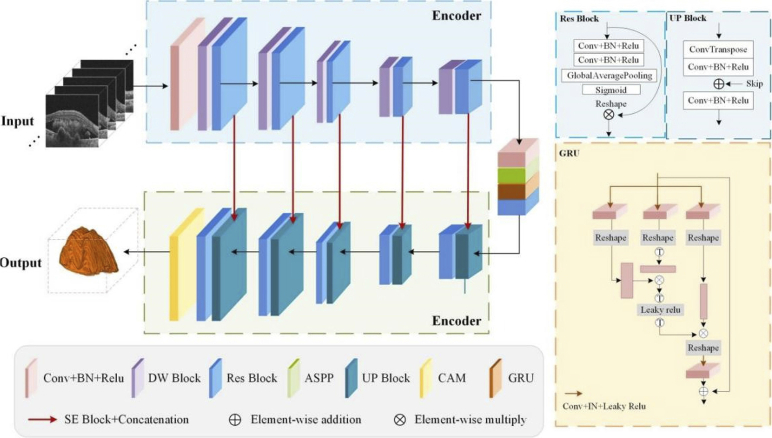
Here we proposed a network characterizing multi-scale and cross-channel feature extraction and channel attention for the 3D segmentation of PEDs in OCT images. As shown in Fig. 1, the backbone image segmentation network is a symmetrical U-shaped structure, including five down-sampling and up-sampling layers with 8, 16, 32, 64, 128, and 256 channels, respectively. The encoder extracts the features and the decoder restores the output to the size of the input image by up-sampling.

Fig. 1.

Schematic overview of the proposed 3D segmentation model.

To improve the accuracy of PEDs 3D segmentation, Atrous Spatial Pyramid Pooling (ASPP) [39], CAM, GRU (Graph Reasoning Units), and SE block [35] were applied in this network. Due to the multi-scale receptive field, the ASPP ensures that more abundant features can be learned as far as possible. The latter two modules make the receptive field cover the whole feature map, strengthen the important channels, and weaken the non-important channels, which is more conducive to the accurate 3D segmentation of lesion areas from the background. Besides, a residual structure [37] is also adopted in the down-sampling of each encoder, which effectively avoids the phenomenon that the final product tends to zero in the forward propagation process following the chain rule because some parameters are too small. What’s more, with the increase in the number of layers, some features will be lost. Introducing a multi-feature map by residual structure can be conducive to the transmission of information. We will detail each module in the proposed model in the following subsections.

The encoding part consists of layers in which each layer combines a down-sampling (DW) module and a Res-block. Each down-sampling module adopts a residual structure in which the first half combines the layers of regular convolutions and Relu activation functions. The other part is still composed of regular convolutions and Relu layers, but the stride of the former convolution is set to 2 for down-sampling, thus halving the size of the feature map. After five layers of down-sampling, the features on the initial image are gradually extracted and a dense low-resolution feature map is produced. Besides, each down-sampling module is followed by a Res-block (seen in Fig. 1), which can avoid the gradient problem caused by the increase in the number of layers and the phenomenon of reduced computing efficiency. Compared with the traditional Res-block [37], a Squeeze-and-Excitation block [35] is first introduced here. This module strengthens the interrelation between channels, to realize the adaptive correction of the intensity of characteristic response between channels.

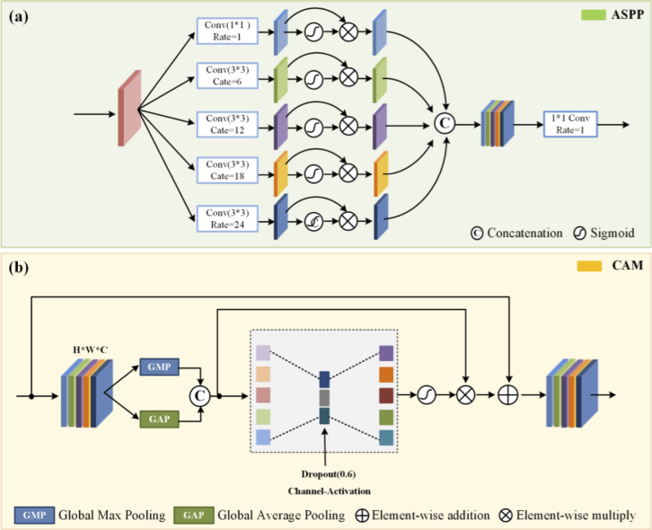
To learn more information about different scales, the ASPP was introduced here. As shown in Fig. 2 (a), ASPP sampled a given input with a series of atrous convolutions with different dilation rates to capture information from an arbitrarily scaled region. Different dilation rates make the size of the receptive field different, and the context information of different sizes can be captured, thus enriching the extracted feature information. Then, the obtained feature maps are concatenated to form the output feature map. What’s more, the GRU can enhance the global reasoning ability. The three branches of this module enable the projection to node space, re-projection to feature space, and the fusion of global features. Therefore, by utilizing these three branches of GRU for projection, disjoint regions or regions that are far apart can be used for global reasoning.

Fig. 2.

The structures of the sub-modules used in this study. (a) is the ASPP (Atrous Spatial Pyramid Pooling), which ensures a rich diversity of extracted information; (b) is the CAM (Channel Attention Mechanism).

At the decoder strategy, an up-sampling module and a Res-block were used. Transposed convolution with the stride of $2\times 2$ was introduced into the decoder instead of a normal up-sampling layer. The feature map after transpose convolution is concatenated with skip connections corresponding to each layer in the encoder, thus integrating the spatial and semantic information, avoiding information loss. At the end of the decoder, a CAM is added to this network to assign the appropriate weight to each channel. It can enhance the features of the region of interest and filter out unnecessary features while maintaining the original features. The detailed structure of CAM is shown in Fig. 2 (b). The original data were processed by global max pooling and global average pooling respectively and then fused by convolution. After the MLP and the sigmoid activation, the new weight matrix was calculated. The original matrix is dotted with the weight matrix to get the redistribution of resources between channels.

2.4. Loss function

One of the major challenges for the segmentation task is that the number of pixels in the diseased area is much lower than at in the non-diseased area. For data imbalance, the learning process may converge to the local minimum of the suboptimal loss function, so segmentation results with high accuracy but a low recall rate may occur. To solve the problem of data imbalance, we use a Tversky loss function [40] to achieve a better balance between precision and recall rate. Tversky loss is derived from the Dice loss function, in which two coefficients $\alpha$ and $\beta$ . are introduced to better balance false negative and false positive. The specific expression of the loss function is as follows.

$$T(\alpha ,\beta )=\frac{{\sum }_{i=1}^N{p}_{0i}{g}_{0i}}{{\sum }_{i=1}^N{p}_{0i}{g}_{0i}+\alpha {\sum }_{i=1}^N{p}_{0i}{g}_{1i}+\beta {\sum }_{i=1}^N{p}_{1i}{g}_{0i}}$$ (1)

where the $p_{0i}$ is the probability of voxel i be a lesion and $p_{1i}$ is the probability of voxel i be a non-lesion. Also, $g_{0i}$ is $1$ for a lesion voxel and $0$ for a non-lesion voxel and vice versa for the $g_{1i}$ . Here, after debugging, we set $\alpha$ to 0.2, and $\beta$ to 0.8.

In addition, due to the small proportion of PEDs in the fundus, the number of pixels between the two types is quite different. Binary cross entropy (BCE) is also introduced here. ${\text{L}}_{\text{BCE}}$ is defined as Eq. (2):

$$L_{\mathit{\text{BCE}}}=-\frac{1}{N}\sum _{\text{i}=1}^N{y}_i.\mathit{\text{log}}(p(y_i))+(1-y_i).\mathit{\text{log}}(1-p(y_i))$$ (2)

where $\text{y }$ is the class label for pixel $\text{i}$ , which is 0 or 1, and $\text{p}(\text{y})$ is the estimated probability of pixel $\text{i}$ belonging to lesions. In this paper, we used a loss function consisting of Tversky loss and binary cross entropy (BCE).

$$L_{\mathit{\text{AMD}}}=\lambda \ast T(\text{α},\text{β})+(1-\text{λ})\ast L_{\mathit{\text{BCE}}},$$ (3)

where λ is a balance parameter that is set as 0.5 for all the experiments.

3. Experiment

3.1. Experimental settings

The original B-scan results all have an initial resolution of $1044\times 512\text{pixels}$ , most regions of which are the dark background. To improve training efficiency and save the cost of time, all images are cropped to $512\times 512\text{pixels}$ and are converted to unit8 format.

The data used for training were enhanced by flipping, rotating, and random vertical or horizontal rolls. Our method was trained with a batch size of 5 using Adam optimizer, with an initial learning rate of 0.0001, which decayed exponentially as the epoch increased. We trained the model for 10 epochs and selected the model with the best metrics on the validation set to save.

The training was performed in a computer with an Intel XeonSilver4210R CPU and 24 cores, using Python 3.9.12 and TensorFlow 2.5.0. On such a set, the training lasted about 15 hours. The testing was also done on the same setup as the training.

The proposed 3D segmentation model is a binary classifier that is supposed to accurately affect areas from the background in B-scan images. The ground-truth images which are annotated by ophthalmologists are used for evaluating the automatic 3D segmentation results. For such a case, the following four parameters are typically involved: False Negative (FN), True Positive (TP), False Positive (FP), and True Negative (TN). Based on the above four parameters, many segmentation metrics are constructed: Pixel Accuracy, Precision, IOU (Intersection over Union), and Dice, for example. Since the results are three-dimensional obtained by the proposed 3D method, the above index used to evaluate the results of traditional two-dimensional segmentation cannot reflect the effect of our results well. Therefore, here we calculated the volume, surface area, and mean distance to surface (MDS) of the 3D segmentation results and compared them with those in the 3D ground truth, which could better reflect the accuracy of the 3D segmentation results.

3.2. Segmentation results and consistency analysis

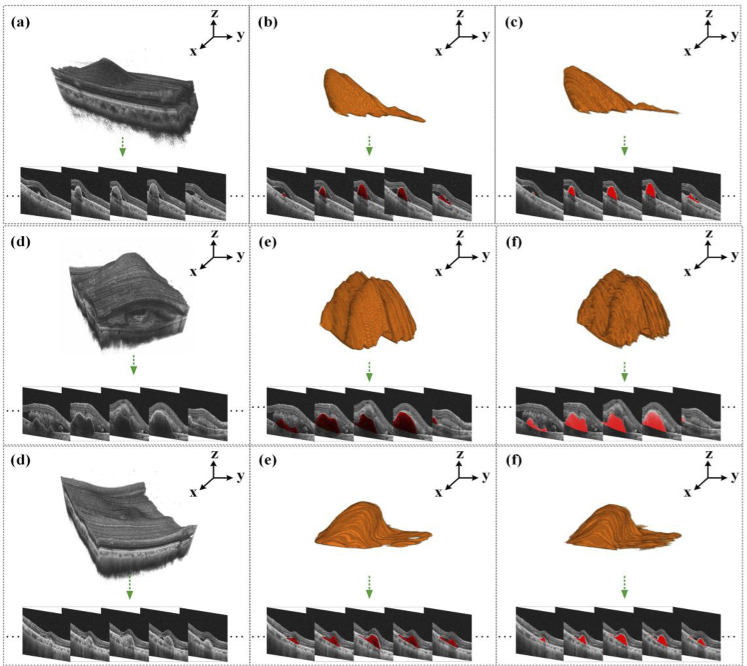
In this section, we demonstrated the results of the above-mentioned experiments to validate our proposed 3D model for PEDs 3D segmentation, as Fig. 3 shows. We further evaluated the 3D segmentation results of the proposed model from the three aspects of volume, surface area, and mean distance to the surface, as shown in Fig. 4 and Fig. 5.

Fig. 3.

Three 3D segmentation results on the selected validation set. From left to right: OCT 3D C-scans consisting of massive B-scans, the 3D segmentation results, and the corresponding manually annotated 3D images.

Fig. 4.

The performance of eight groups of data in volume, surface area, and MDS.

Fig. 5.

Bland-Altman agreement analysis of wet AMD against measurements, where the solid blue line represents the bias, and the dashed blue lines represent the upper and lower 95% limits of agreement.

Figure 3 shows the original OCT image (the left), the predicted 3D lesion image (the middle), and the 3D lesion image manually annotated by ophthalmologists (the right). It can be seen intuitively that the 3D prediction results can be close to the actual morphology of the lesion, which is helpful for ophthalmologists to accurately judge the progression of wet AMD. To evaluate these 3D segmentation results, we separately calculated the volume, surface area, and mean distance to surface (MDS) of 33 groups of 3D segmentation results and their corresponding ground truth. The specific results are shown in Fig. 4.

Figure 4 shows the quantitative scatter plots of the volume, areas, and MDS (Mean Distance to surface) measurements of PEDs along with Pearson’s correlation analyses for the proposed algorithm vs. the manual segmentation, respectively. The red lines represent the fit of these scattered points. Figure 4 (a) shows a significant correlation between the measurements of PEDs (r = 0.99753, p < 0.0001), as do the results in Fig. 4 (b) (r = 0.99628, p < 0.0001) and Fig. 4 (c) (r = 0.99879, p < 0.0001). The result of automatic 3D segmentation is compared with that of manual segmentation, and Bland-Altman analysis showed that the average bias of the volume measurements was $-0.21048\text{m}{\text{m}}^3$ (95% limits of agreement [-0.93074, 0.50977], Fig. 5 (a)) and the average bias of the area surface measurements was $8.48383\text{m}{\text{m}}^2$ (95% limits of agreement [-16.10051, 33.06817], Fig. 5 (b)). For MDS, the average bias was $-0.03121\text{mm}$ . (95% limits of agreement [-0.12081, 0.05839], Fig. 5 (c)). the model performs well in the three indicators of volume, surface area, and MDS, which is of great value for clinical diagnosis of wet AMD progression. By observing Fig. 4 and Fig. 5, it can be found that the volume and MDS of the segmentation results had little difference from the actual manual labeling results, but the measured surface area is relatively small. The deviation value increased with the size of the lesion.

3.3. ternal testing

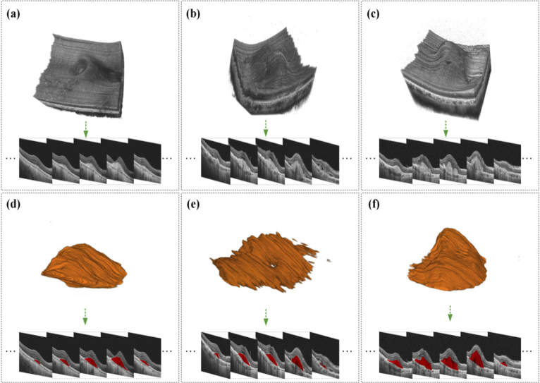
To ensure the rigor of our experiment, we randomly selected three groups of data in the datasets for testing. Figure 6 shows the new 3D segmentation results predicted by the proposed 3D segmentation model. Figure 6 shows the 3D segmentation results of three lesions from left to right. The first row is the original image to be segmented corresponding to each data and its corresponding b-scan image. Input them into our network for 3D segmentation, and the results are respectively shown in Fig. 6 (d-f). As can be seen from the picture, the external test results not only achieved a relatively accurate segmentation effect on the two-dimensional level but also clearly showed the 3D shapes of the lesions in the final 3D results. The 3D segmentation results are detailed in the Supplementary Materials (Visualization 1 ^{(21.3MB, avi)} , Visualization 2 ^{(2.4MB, avi)} , Visualization 3 ^{(1.4MB, avi)} , Visualization 4 ^{(32.4MB, avi)} , Visualization 5 ^{(2.8MB, avi)} , Visualization 6 ^{(1.8MB, avi)} , Visualization 7 ^{(23.7MB, avi)} , Visualization 8 ^{(2.4MB, avi)} and Visualization 9 ^{(1.7MB, avi)} ).

Fig. 6.

PEDs 3D segmentation results on three new datasets. (a) - (b) OCT 3D B-scans consisting of massive B-scans, (d) - (f) corresponding PEDs 3D segmentation results (see Visualization 1 ^{(21.3MB, avi)} , Visualization 2 ^{(2.4MB, avi)} , Visualization 3 ^{(1.4MB, avi)} , Visualization 4 ^{(32.4MB, avi)} , Visualization 5 ^{(2.8MB, avi)} , Visualization 6 ^{(1.8MB, avi)} , Visualization 7 ^{(23.7MB, avi)} , Visualization 8 ^{(2.4MB, avi)} and Visualization 9 ^{(1.7MB, avi)} ).

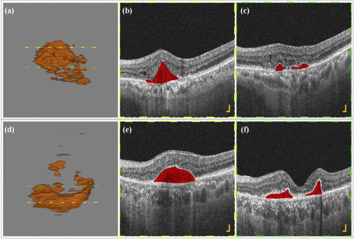
Figure 7 and Supplementary Materials (Visualization 10 ^{(1.6MB, avi)} , Visualization 11 ^{(32.4MB, avi)} , Visualization 12 ^{(2.9MB, avi)} , Visualization 13 ^{(1.9MB, avi)} , Visualization 14 ^{(33.2MB, avi)} and Visualization 15 ^{(2.3MB, avi)} ) show the 3D segmentations of two PEDs lesions and their corresponding B-scan images. Figure 7 (b) and (c) correspond to the B-scan images at the yellow dotted line in Fig. 7 (a) and Fig. 7 (d), whale Fig. 7 (c) and Fig. 7 (f) correspond to the B-scan image at the green dotted line in Fig. 7 (a) and Fig. 7 (d). It can be observed that the 3D shape of PEDs lesions is irregular, and some patients may have more than one lesion area, which is difficult to obtain by the traditional two-dimensional segmentation method. The number of PEDs lesions is sometimes not only one but several nearby areas. In clinical practice, conservative observation is often employed in this situation, regular examination, once the visual impairment is found, immediate treatment and intervention are given. However, Ophthalmologists can only infer whether there are other small lesions nearby based on B-scan images and two-dimensional fundus angiography, which makes it easy to miss some potential small lesions that may impair vision in the future. Here the 3D segmentation results can show the 3D morphology of all the lesions in the area and meanwhile, preserve B-scan images, which can help retina specialists accurately evaluate the lesion situations, and further improve corresponding diagnosis and treatment.

Fig. 7.

PEDs 3D segmentation results (a) - (d) and corresponding B-scan images (b) - (c), (e) - (f) of two patients with wet AMD (see Visualization 10 ^{(1.6MB, avi)} , Visualization 11 ^{(32.4MB, avi)} , Visualization 12 ^{(2.9MB, avi)} , Visualization 13 ^{(1.9MB, avi)} , Visualization 14 ^{(33.2MB, avi)} and Visualization 15 ^{(2.3MB, avi)} ). All scale bars are 200 μm.

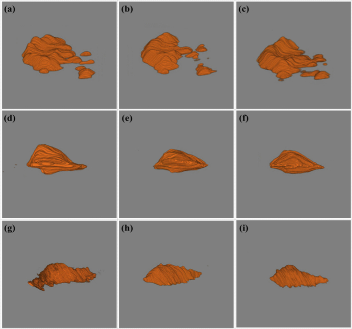
Based on the above, we introduced more 3D OCT images for the 3D segmentation test to demonstrate the performance of our 3D segmentation model and show more 3D shape differences of PEDs in patients. The corresponding results are shown in Fig. 8 and Supplementary Materials (Visualization 16 ^{(1.4MB, avi)} , Visualization 17 ^{(2.6MB, avi)} , Visualization 18 ^{(1.6MB, avi)} , Visualization 19 ^{(2.9MB, avi)} , Visualization 20 ^{(1.5MB, avi)} , Visualization 21 ^{(2.9MB, avi)} , Visualization 22 ^{(1.5MB, avi)} , Visualization 23 ^{(2MB, avi)} , Visualization 24 ^{(1.1MB, avi)} , Visualization 25 ^{(3.6MB, avi)} , Visualization 26 ^{(1.5MB, avi)} , Visualization 27 ^{(3MB, avi)} , Visualization 28 ^{(1.3MB, avi)} , Visualization 29 ^{(3.2MB, avi)} , Visualization 30 ^{(1.2MB, avi)} , Visualization 31 ^{(2.9MB, avi)} , Visualization 32 ^{(1.3MB, avi)} and Visualization 33 ^{(2.8MB, avi)} ). Those nine 3D images are all from different wet AMD patients. From Fig. 8, it can be observed that the 3D shapes and the sizes of different wet AMD patients were different, which can help retina specialists understand AMD diseases better. Those 3D segmentation results have demonstrated that our 3D segmentation model has good adaptability and high robustness to different 3D AMD lesion shapes, and it was also the first time that different 3D shapes of PEDs have been present. It may provide a great convenience for clinical ophthalmologists to diagnose, monitor, and assess wet AMD.

Fig. 8.

Subretinal hyperreflective material 3D segmentation results of nine patients show the differences in shape, size, and surface details (see Visualization 16 ^{(1.4MB, avi)} , Visualization 17 ^{(2.6MB, avi)} , Visualization 18 ^{(1.6MB, avi)} , Visualization 19 ^{(2.9MB, avi)} , Visualization 20 ^{(1.5MB, avi)} , Visualization 21 ^{(2.9MB, avi)} , Visualization 22 ^{(1.5MB, avi)} , Visualization 23 ^{(2MB, avi)} , Visualization 24 ^{(1.1MB, avi)} , Visualization 25 ^{(3.6MB, avi)} , Visualization 26 ^{(1.5MB, avi)} , Visualization 27 ^{(3MB, avi)} , Visualization 28 ^{(1.3MB, avi)} , Visualization 29 ^{(3.2MB, avi)} , Visualization 30 ^{(1.2MB, avi)} , Visualization 31 ^{(2.9MB, avi)} , Visualization 32 ^{(1.3MB, avi)} and Visualization 33 ^{(2.8MB, avi)} ).

3.4. Comparison experiment

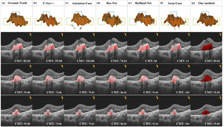
To demonstrate the advantage of our proposed method in terms of wet AMD segmentation, we compared it with five segmentation methods (U-Net++ [41], Attention-U-Net [42], Residual-U-Net (Res-Net) [43], Retfluid-Net [28], Swin-U-Net [44]). All of these networks were applied to the 2D segmentation of retinal diseases. Therefore, here we integrated those methods into our architecture for comparison testing. The experimental results of our method and other competitors on a typical case are illustrated in Fig. 9. As shown in Fig. 9, most methods can generate 3D results, however, for PEDs segmentation, the competitors often produce fragments that do not belong to lesions and segmentation accuracy, such as the results obtained by Attention-U-Net in Fig. 9.

Fig. 9.

PEDs segmentation results of our model are compared to five existing methods. (b) - (g) PEDs 3D segmentation results. The unit of data in the lower right corner is pixel. All the scale bars are 200 µm.

To distinguish the segmentation results obtained by several methods more easily, we selected three representative parts for emphasis comparison (seen in the green, blue, and yellow boxes). In terms of the overall morphology, the segmentation results of each method are relatively close, but in some details, such as the green, blue, and yellow boxes, the performance of each network is different. Clinically, the CMT index is often generally used to measure the condition of AMD. In this experiment, we also adopted this metric to compare our results with the segmentation results of other competitors. Three local B-scan results of this sample are selected to measure their CMT index, the results of which are presented in the lower right corner of each figure in sections. It can be seen that the results obtained by our method are the closest to Ground Truth in the data of the three b-scans, which further proves the accuracy of the segmentation method.

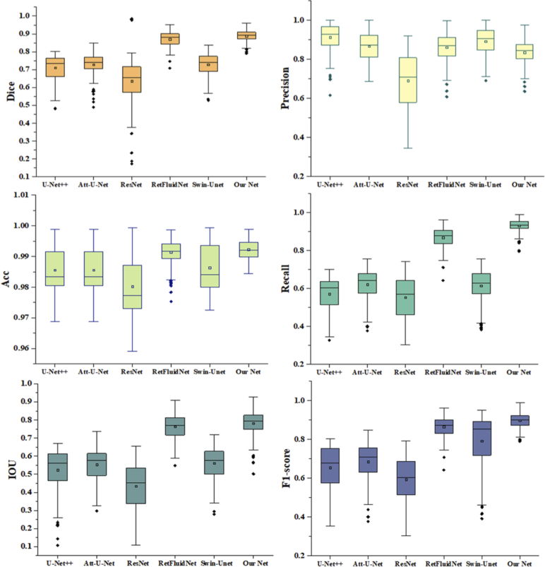
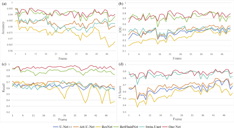
In addition, the above 3D segmentation results were quantitatively evaluated from five perspectives, including Dice, Precision, Accuracy, Recall, IOU, and F1-score. The boxplots of different results are depicted in Fig. 10. It can be intuitively seen that the results obtained by our segmentation method had excellent segmentation effects. Among these five metrics, the variance of our results can reach the minimum, and the range of upper and lower limits is small, indicating that our results data is relatively concentrated and stable. Here, we showed the performance of each frame of this sample on four metrics, Dice, IOU, F1-score, and Recall, as shown in Fig. 11. It can be seen that our segmentation results, represented by the red solid line, performed better than other segmentation results on all four metrics, which means that our results are closest to the labels.

Fig. 10.

Box plot of six segmentation results on Dice, Precision, Accuracy, Recall, IOU, and F1-score.

Fig. 11.

The frame-by-frame performance of the segmentation results obtained by each network on four metrics.

The specific data are shown in Table 1. It can be observed that in all experiments, our method outperforms other methods, which proves the contribution of the proposed model. As seen, the average Dice, Precision, Accuracy, Recall, IOU, and F1-score of our methods achieve 0.850, 0.835, 0.992, 0.931, 0.790, and 0.759 respectively, which convincingly demonstrate that our net is effective in AMD segmentation.

Table 1. Quantitative results of different methods in PEDs segmentation.

Method	U-Net++	Att-U-Net	ResNet	RetfluidNet	Swin-Unet	Our method
Dice	0.675 ± 0.234	0.650 ± 0.233	0.556 ± 0.262	0.713 ± 0.154	0.785 ± 0.183	0.850 ± 0.137
Precision	0.913 ± 0.222	0.868 ± 0.277	0.692 + 0.296	0.861 + 0.206	0.892 ± 0.173	0.835 ± 0.147
Accuracy	0.986 ± 0.007	0.986 ± 0.007	0.980 ± 0.010	0.991 ± 0.004	0.986 ± 0.008	0.992 ± 0.003
Recall	0.599 ± 0.210	0.638 ± 0.202	0.555 ± 0.242	0.873 ± 0.083	0.616 ± 0.185	0.931 ± 0.128
IOU	0.535 ± 0.204	0.562 ± 0.202	0.448 ± 0.206	0.767 ± 0.181	0.562 ± 0.172	0.790 ± 0.171
F1-score	0.526 ± 0.225	0.548 ± 0.225	0.426 ± 0.247	0.741 ± 0.151	0.615 ± 0.178	0.759 ± 0.136

3.5. Ablation experiments

In order to justify the effectiveness of the SE block, CAM, and GRU in the proposed model, we conduct the following ablation experiments. Our proposed method is based on U-Net, therefore we set U-Net as the most fundamental baseline model. We replace the proposed blocks with regular convolution operations, aiming at enhancing the learning capability. We then incorporated each block into the baseline to get Model1, Model2, and Model3, as shown in Table 2. To further verify the effectiveness of these modules, we combined them in pairs and tested three groups in total. The last column in Table 2 shows the segmentation effect of the network with all modules. It can be shown that the backbone net achieved a better performance by adopting our proposed blocks.

Table 2. Ablation experiment results over our dataset.

Network	Module			Metrics
	SE	CAM	GRU	Precision	Dice	Accuracy	Jaccard	IOU
Baseline				52.6 ± 11.72	67.75 ± 11.77	97.03 ± 1.51	52.26 ± 11.69	52.27 ± 11.67
Model 1	√			55.54 ± 15.26	69.81 ± 14.77	97.62 ± 0.92	55.33 ± 15.2	55.34 ± 15.19
Model 2		√		60.19 ± 13.36	73.25 ± 12.77	97.90 ± 0.99	59.12 ± 13.4	59.13 ± 13.39
Model 3			√	66.49 ± 14.9	77.33 ± 13.17	98.42 ± 0.81	64.63 ± 15.05	64.64 ± 15.03
Model 4	√	√		66.55 ± 15.76	77.53 ± 14.83	98.44 ± 0.81	65.18 ± 15.65	65.19 ± 15.63
Model 5	√		√	68.76 ± 15.16	77.94 ± 12.71	98.47 ± 0.75	73.44 ± 12.36	65.29 ± 13.81
Model 6		√	√	60.18 ± 13.19	76.43 ± 10.37	98.9 ± 0.86	67.11 ± 13.24	62.13 ± 13.25
Model 7	√	√	√	85.7 ± 11.56	89.12 ± 11.87	99.42 ± 0.42	81.45 ± 11.55	81.85 ± 13.77

4. Clinical trial results

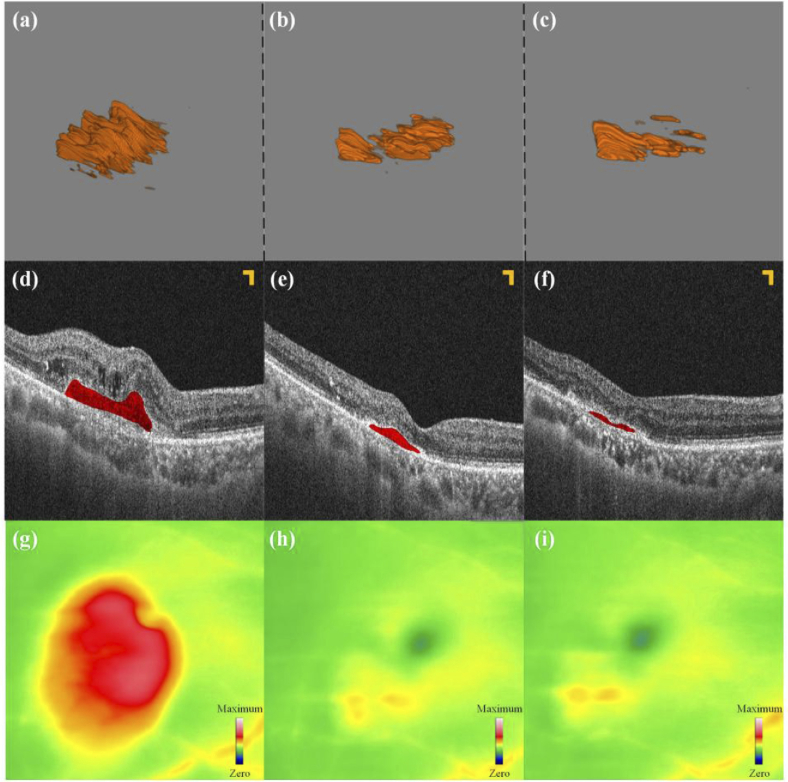
Figure 12 depicts the treatment progress of this wet AMD patient for four months, during which the patient received three intravitreal injections. These pictures were arranged by time from left to right, representing different stages of treatment. Before initial treatment, the patient’s best-corrected visual acuity (BCVA) was 20/133. OCT scanning (seen in Fig. 12 (a)) revealed an increase in central macular thickness (CMT), significant PEDs lesions, and signs of CNV and intraretinal fluid (IRF). After two initial injections, follow-up at one-month intervals showed that the patient’s BCVA remained at 20/133, the CMT decreased significantly compared to before, PEDs lesions significantly reduced, the blood flow signals of the CNV weakened, and the IRF disappeared (as seen in Fig. 12 (b, e, h)). After completing three initial treatments, the patient underwent a review 30 days later. His BCVA improved to 20/80, and OCT (seen in Fig. 12 (c)) showed a further reduction in CMT, a significant decrease in lesion volume, partial regression of the CNV, and a weakening of blood flow signals.

Fig. 12.

PEDs 3D segmentation results. (a) - (c): The 3D segmentation results. (d) - (f): B-scan images corresponding to the same section. (g - i): The corresponding thickness map of (a) - (c). All scale bars are 200 µm.

Figure 12(d-f) show B-scan images of this sample at the fovea at three examinations. Figure 12(g-i) show the thickness topography of the boundary membrane to Bruch’s membrane in the three stages. The green and yellow parts represent the thickness at the normal value and critical value, respectively. However, the red part indicates that the part is thicker than the normal range, and the redder the color, the thicker the thickness. Both kinds of results prove that the above 3D segmentation results are accurate.

The above experiment shows that the changes in fundus conditions in the patient with wet AMD can be intuitively and properly reflected in the 3D segmentation results. Besides, the 3D segmentation results are consistent with the diagnostic results obtained by the existing clinical diagnostic means, and can further provide more comprehensive information on wet AMD. Therefore, our method can provide great convenience for the diagnosis and follow-up of the therapeutic effect of wet AMD, while increasing the acceptance and recognition of the diagnosis results in the clinical patients. The 3D segmentation results of wet AMD lesions can also help retina specialists communicate with the patients by showing the patients more visual information.

5. Conclusion

A deep learning-based model for 3D segmentation of PEDs on OCT images was developed and evaluated. Experiments conducted on our PEDs OCT datasets demonstrated that our model can achieve excellent 3D segmentation results of PEDs, which probably holds great promise in providing the precision and efficiency of ophthalmic disease.

Compared with the existing two-dimensional segmentation methods, our method achieved a remarkable 3D segmentation performance, and different 3D shape features of PEDs have been shown and measured for the first time, such as 3D surface areas and volumes. 3D lesion information can help understand ophthalmic diseases better and improve corresponding diagnosis and treatment. With 3D visualization features, 3D segmentation of PEDs assisted by artificial intelligence can serve as a powerful tool for diagnosing and monitoring wet AMD, potentially alleviating the time-consuming manual image reading, with 3D quantitative lesion information. This achievement may bring great convenience for the clinical diagnosis and treatment of wet AMD due to the visual interpretability for ophthalmologists’ decision-making, thus facilitating the formulation of a therapeutic schedule.

Funding

National Natural Science Foundation of China10.13039/501100001809 (61905036); China Postdoctoral Science Foundation10.13039/501100002858 (2021T140090, 2019M663465); Fundamental Research Funds for the Central Universities10.13039/501100012226 (University of Electronic Science and Technology of China) (ZYGX2021J012); Medico-Engineering Cooperation Funds from University of Electronic Science and Technology of China10.13039/501100005408 (ZYGX2021YGCX019); Key Research and Development Project of Health Commission of Sichuan Province10.13039/501100020207 (ZH2024-201).

Disclosures

The authors declare no conflicts of interest.

Data availability

Data underlying the results presented in this paper are not publicly available at this time but may be obtained from the authors upon reasonable request.

References

- 1.Brandl C., Günther F., Zimmermann M. E., et al. , “Incidence, progression and risk factors of age-related macular degeneration in 35–95-year-old individuals from three jointly designed German cohort studies,” BMJ Open Ophth. 7(1), e000912 (2022). 10.1136/bmjophth-2021-000912 [DOI] [PMC free article] [PubMed] [Google Scholar]
- 2.Wang Z., Sadda S. R., Lee A., et al. , “Automated segmentation and feature discovery of age-related macular degeneration and Stargardt disease via self-attended neural networks,” Sci. Rep. 12(1), 14565 (2022). 10.1038/s41598-022-18785-6 [DOI] [PMC free article] [PubMed] [Google Scholar]
- 3.Mendonça L. S. M., Levine E. S., Waheed N. K., “Can the Onset of Neovascular Age-Related Macular Degeneration Be an Acceptable Endpoint for Prophylactic Clinical Trials?” Ophthalmologica 244(5), 379–386 (2021). 10.1159/000513083 [DOI] [PubMed] [Google Scholar]
- 4.Sutton J., Menten M. J., Riedl S., et al. , “Correction: Developing and validating a multivariable prediction model which predicts progression of intermediate to late age-related macular degeneration—the PINNACLE trial protocol,” Eye 37(6), 1275–1283 (2022). 10.1038/s41433-022-02097-0 [DOI] [PMC free article] [PubMed] [Google Scholar]
- 5.Lim L. S., Mitchell P., Seddon J. M., et al. , “Age-related macular degeneration,” Lancet 379(9827), 1728–1738 (2012). 10.1016/S0140-6736(12)60282-7 [DOI] [PubMed] [Google Scholar]
- 6.Li J. Q., Welchowski T., Schmid M., et al. , “Prevalence and incidence of age-related macular degeneration in Europe: a systematic review and meta-analysis,” Br. J. Ophthalmol. 104(8), 1077–1084 (2020). 10.1136/bjophthalmol-2019-314422 [DOI] [PubMed] [Google Scholar]
- 7.Wong W. L., Su X., Li X., et al. , “Global prevalence of age-related macular degeneration and disease burden projection for 2020 and 2040: a systematic review and meta-analysis,” Lancet Global Health 2(2), e106–e116 (2014). 10.1016/S2214-109X(13)70145-1 [DOI] [PubMed] [Google Scholar]
- 8.Ganjdanesh A., Zhang J., Chew E. Y., et al. , “LONGL-Net: temporal correlation structure guided deep learning model to predict longitudinal age-related macular degeneration severity,” PNAS Nexus 1(1), pgab003 (2022). 10.1093/pnasnexus/pgab003 [DOI] [PMC free article] [PubMed] [Google Scholar]
- 9.Au A., Santina A., Abraham N., et al. , “Relationship Between Drusen Height and OCT Biomarkers of Atrophy in Non-Neovascular AMD,” Invest. Ophthalmol. Visual Sci. 63(11), 24 (2022). 10.1167/iovs.63.11.24 [DOI] [PMC free article] [PubMed] [Google Scholar]
- 10.Bird A. C., Bressler N. M., Bressler S. B., et al. , “An international classification and grading system for age-related maculopathy and age-related macular degeneration. The International ARM Epidemiological Study Group,” Surv. Ophthalmol. 39(5), 367–374 (1995). 10.1016/S0039-6257(05)80092-X [DOI] [PubMed] [Google Scholar]
- 11.Altay L., Scholz P., Schick T., et al. , “Association of Hyperreflective Foci Present in Early Forms of Age-Related Macular Degeneration With Known Age-Related Macular Degeneration Risk Polymorphisms,” Invest. Ophthalmol. Vis. Sci. 57(10), 4315–4320 (2016). 10.1167/iovs.15-18855 [DOI] [PubMed] [Google Scholar]
- 12.Stahl A., “The Diagnosis and Treatment of Age-Related Macular Degeneration,” Dtsch Arztebl International 117, 513–519 (2020). 10.3238/arztebl.2020.0513 [DOI] [PMC free article] [PubMed] [Google Scholar]
- 13.Elsharkawy M., Elrazzaz M., Ghazal M., et al. , “Role of Optical Coherence Tomography Imaging in Predicting Progression of Age-Related Macular Disease: A Survey,” Diagnostics 11(12), 2313 (2021). 10.3390/diagnostics11122313 [DOI] [PMC free article] [PubMed] [Google Scholar]
- 14.Loughman J., Sabour-Pickett S., Nolan J. M., et al. , “Visual Function and Its Relationship with Severity of Early, and Activity of Neovascular, Age-Related Macular Degeneration,” J. Clin. Exp. Ophthalmol. 06(05), 488 (2015). 10.4172/2155-9570.1000488 [DOI] [PMC free article] [PubMed] [Google Scholar]
- 15.Sassa Y., Hata Y., “Antiangiogenic drugs in the management of ocular diseases: Focus on antivascular endothelial growth factor,” Clin. Ophthalmol. 4, 275–283 (2010). 10.2147/opth.s6448 [DOI] [PMC free article] [PubMed] [Google Scholar]
- 16.Karampelas M., Malamos P., Petrou P., et al. , “Retinal Pigment Epithelial Detachment in Age-Related Macular Degeneration,” Ophthalmol Ther. 9(4), 739–756 (2020). 10.1007/s40123-020-00291-5 [DOI] [PMC free article] [PubMed] [Google Scholar]
- 17.Bird A. C., Marshall J., “Retinal pigment epithelial detachments in the elderly,” Trans. Ophthalmol. Soc. 105(Pt 6), 674–682 (1986). [PubMed] [Google Scholar]
- 18.Poliner L. S., Olk R. J., Burgess D., et al. , “Natural history of retinal pigment epithelial detachments in age-related macular degeneration,” Ophthalmology 93(5), 543–551 (1986). 10.1016/S0161-6420(86)33703-5 [DOI] [PubMed] [Google Scholar]
- 19.Yannuzzi L. A., Sorenson J., Spaide R. F., et al. , “Idiopathic polypoidal choroidal vasculopathy (IPCV),” Retina 10(1), 1–8 (1990). 10.1097/00006982-199010010-00001 [DOI] [PubMed] [Google Scholar]
- 20.Pauleikhoff D., Löffert D., Spital G., et al. , “Pigment epithelial detachment in the elderly. Clinical differentiation, natural course and pathogenetic implications,” Graefe’s Arch. Clin. Exp. Ophthalmol. 240(7), 533–538 (2002). 10.1007/s00417-002-0505-8 [DOI] [PubMed] [Google Scholar]
- 21.Fazekas B., Lachinov D., Aresta G., et al. , “Segmentation of Bruch’s Membrane in retinal OCT with AMD using anatomical priors and uncertainty quantification,” IEEE J. Biomed. Health Inform. 27(1), 41–52 (2022). 10.1109/JBHI.2022.3217962 [DOI] [PubMed] [Google Scholar]
- 22.Massatsch P., Charrière F., Cuche E., et al. , “Time-domain optical coherence tomography with digital holographic microscopy,” Appl. Opt. 44(10), 1806–1812 (2005). 10.1364/AO.44.001806 [DOI] [PubMed] [Google Scholar]
- 23.Huang D., Swanson E. A., Lin C. P., et al. , “Optical Coherence Tomography,” Science 254(5035), 1178–1181 (1991). 10.1126/science.1957169 [DOI] [PMC free article] [PubMed] [Google Scholar]
- 24.Hee M. R., Izatt J. A., Swanson E. A., et al. , “Optical coherence tomography of the human retina,” Arch. Ophthalmol. 113(3), 325–332 (1995). 10.1001/archopht.1995.01100030081025 [DOI] [PubMed] [Google Scholar]
- 25.Rastogi V., Agarwal S., Dubey S. K., et al. , “Design and development of volume phase holographic grating based digital holographic interferometer for label-free quantitative cell imaging,” Appl. Opt. 59(12), 3773–3783 (2020). 10.1364/AO.387620 [DOI] [PubMed] [Google Scholar]
- 26.Wintergerst M. W. M., Schultz T., Birtel J., et al. , “Algorithms for the Automated Analysis of Age-Related Macular Degeneration Biomarkers on Optical Coherence Tomography: A Systematic Review,” Trans. Vis. Sci. Tech. 6(4), 10 (2017). 10.1167/tvst.6.4.10 [DOI] [PMC free article] [PubMed] [Google Scholar]
- 27.Scharf J., Corradetti G., Corvi F., et al. , “Optical Coherence Tomography Angiography of the Choriocapillaris in Age-Related Macular Degeneration,” J. Clin. Med. 10(4), 751 (2021). 10.3390/jcm10040751 [DOI] [PMC free article] [PubMed] [Google Scholar]
- 28.Sappa L. B., Okuwobi I. P., Li M., et al. , “RetFluidNet: Retinal Fluid Segmentation for SD-OCT Images Using Convolutional Neural Network,” J. Digit. Imaging. 34(3), 691–704 (2021). 10.1007/s10278-021-00459-w [DOI] [PMC free article] [PubMed] [Google Scholar]
- 29.Shen Y., Li J., Zhu W., et al. , “Graph Attention U-Net for Retinal Layer Surface Detection and Choroid Neovascularization Segmentation in OCT Images,” IEEE Trans. Med. Imaging 42(11), 3140–3154 (2023). 10.1109/TMI.2023.3240757 [DOI] [PubMed] [Google Scholar]
- 30.Suchetha M., Ganesh N. S., Raman R., et al. , “Region of interest-based predictive algorithm for subretinal hemorrhage detection using faster R-CNN,” Soft. Computing 25(24), 15255–15268 (2021). 10.1007/s00500-021-06098-1 [DOI] [PMC free article] [PubMed] [Google Scholar]
- 31.Moradi M., Chen Y., Du X., et al. , “Deep ensemble learning for automated non-advanced AMD classification using optimized retinal layer segmentation and SD-OCT scans,” Comput. Biol. Med. 154, 106512 (2023). 10.1016/j.compbiomed.2022.106512 [DOI] [PubMed] [Google Scholar]
- 32.De Fauw J., Ledsam J. R., Romera-Paredes B., et al. , “Clinically applicable deep learning for diagnosis and referral in retinal disease,” Nat. Med. 24(9), 1342–1350 (2018). 10.1038/s41591-018-0107-6 [DOI] [PubMed] [Google Scholar]
- 33.Moraes G., Fu D. J., Wilson M., et al. , “Quantitative Analysis of OCT for Neovascular Age-Related Macular Degeneration Using Deep Learning,” Ophthalmology 128(5), 693–705 (2021). 10.1016/j.ophtha.2020.09.025 [DOI] [PMC free article] [PubMed] [Google Scholar]
- 34.Ronneberger O., Fischer P., Brox T., “U-Net: Convolutional Networks for Biomedical Image Segmentation,” in Medical Image Computing And Computer-Assisted Intervention, Pt III, (2015), pp. 234–241. [Google Scholar]
- 35.Hu J., Shen L., Albanie S., et al. , “Squeeze-and-Excitation Networks,” IEEE Trans. Pattern Anal. Mach. Intell. 42(8), 2011–2023 (2020). 10.1109/TPAMI.2019.2913372 [DOI] [PubMed] [Google Scholar]
- 36.Wang L., Shen B., Zhao N., et al. , “Is the skip connection provable to reform the neural network loss landscape?” in Proceedings of the Twenty-Ninth International Joint Conference on Artificial Intelligence, (Yokohama, Yokohama, Japan, 2021), p. Article 387. [Google Scholar]
- 37.He K., Zhang X., Ren S., et al. , “Deep Residual Learning for Image Recognition,” in 2016 IEEE Conference on Computer Vision and Pattern Recognition (CVPR), (2016), 770–778. [Google Scholar]
- 38.Woo S., Park J., Lee J.-Y., et al. , “CBAM: Convolutional Block Attention Module,” in Computer Vision – ECCV 2018, (Springer International Publishing, 2018), 3-19. [Google Scholar]
- 39.Yang C., Lu G. M., “Skin Lesion Segmentation with Codec Structure Based Upper and Lower Layer Feature Fusion Mechanism,” Ksii Transactions On Internet And Information Systems 16, 60–79 (2022). [Google Scholar]
- 40.Salehi S. S. M., Erdogmus D., Gholipour A., “Tversky Loss Function for Image Segmentation Using 3D Fully Convolutional Deep Networks,” in Machine Learning In Medical Imaging (MLMI 2017), (2017), pp. 379–387. [Google Scholar]
- 41.Zhou Z., Siddiquee M. Mahfuzur Rahman, Tajbakhsh N., et al. , “UNet++: Redesigning Skip Connections to Exploit Multiscale Features in Image Segmentation,” arXiv, (2020). 10.48550/arXiv.1912.05074 [DOI] [PMC free article] [PubMed]
- 42.Oktay O., Schlemper J., Folgoc L. L., et al. , “Attention U-Net: Learning Where to Look for the Pancreas,” arXiv, (2018). 10.48550/arXiv.1804.03999 [DOI]
- 43.Diakogiannis F. I., Waldner F., Caccetta P., et al. , “ResUNet-a: A deep learning framework for semantic segmentation of remotely sensed data,” ISPRS Journal of Photogrammetry and Remote Sensing 162, 94–114 (2020). 10.1016/j.isprsjprs.2020.01.013 [DOI] [Google Scholar]
- 44.Cao H., Wang Y., Chen J., et al. , “Swin-Unet: Unet-Like Pure Transformer for Medical Image Segmentation,” in Computer Vision – ECCV 2022 Workshops: Tel Aviv, Israel, October 23–27, 2022, Proceedings, Part III, (Springer-Verlag, Tel Aviv, Israel, 2023), pp. 205–218. [Google Scholar]
Associated Data
This section collects any data citations, data availability statements, or supplementary materials included in this article.
Data Availability Statement