Simple Approaches for Dealing With Correlated Data

Correlated data refers to a situation where the outcome of interest is clustered within a particular grouping, and they are very common in epidemiology and public health research. Here, we discuss situations that lead to, and complications that result from, correlated data. We demonstrate 2 simple strategies that can be used to analyze correlated data and still obtain valid inferences.

Correlated data arise as the result of dependent sampling. Correlations among model covariates (i.e., independent variables) can result in collinearity problems, but we focus here on correlated outcomes. Examples scenarios include:

1. Pregnancy outcomes (e.g., preterm birth) may be correlated if some or all women in the sample contribute several pregnancies to the data set.

2. Surgery outcomes (e.g., hip replacement) may be correlated if surgeons perform several surgeries for different people in the data set.

3. Any outcome (e.g., cardiovascular, neurologic, renal, pregnancy) will likely be correlated if the outcomes are measured repeatedly over follow-up on the same person.

4. Outcomes in neighborhood-based studies will typically be subject to correlated outcomes because of self-selection and shared features of the social and built environment.

Problems with correlated outcomes arise because of how parameters are estimated. Suppose interest lies in the following linear model:

where, for example, represents blood lead concentration, and is an indicator of being randomized to take a new drug for reducing blood lead (versus placebo). Suppose further that we fit this model to the fabricated data in Table 1 (with only 3 observations, for simplicity).

Table 1.

Hypothetical Data With 3 Observations and 2 Variables, Blood Lead Concentration and an Indicator of Whether an Individual Took an Experimental Drug (Versus Placebo)

Subject No.	Blood Lead Result	Experimental Drug Identifier
1	221.0	0
2	132.7	1
3	125.8	1

Typically, the objective would be to estimate β₁, which could be interpreted as a difference in average blood lead concentrations between the treated and placebo groups. One common approach to estimating this parameter is maximum likelihood estimation (although other similar methods would share the same problems) (1). For the model above, maximum likelihood estimation proceeds by specifying a likelihood for each person in the data and multiplying these likelihoods to obtain the joint likelihood of y:

Software programs typically find the values of β₀ and β₁ that maximize the joint likelihood given the data (1). Although likelihoods are not probabilities, they factor in the same way. Thus, just as only if A₁, A₂,and A₃ are independent (not correlated), so too can the above joint likelihood factorize if the outcomes y are independent.

If the outcomes are correlated, one cannot break up the joint likelihood into the product of individual likelihoods, and special consideration is needed to modify the estimation approach. One key consequence of correlated outcomes is systematic underestimation of the standard errors. Conceptually, each individual’s unique (independent) contribution to the data is diluted by the correlation with others’ contributions. When estimating standard errors, this results in less overall information in the sample, and the need to adjust standard errors accordingly.

The same is true whether one uses likelihood-based methods or other approaches (e.g., ordinary least squares). Using real data, we look at 2 simple methods to handle such situations: robust variance estimation and the clustered bootstrap.

One common misconception is that the presence of correlated outcome data requires the use of generalized estimating equations (GEE) or mixed effects models. This is not true. If the question of interest entails understanding the correlation structure, one may opt to use GEE, second-order GEE, or mixed effects models (2). However, if interest lies only in valid point estimates and valid standard errors in the presence of correlated outcomes, GEE or mixed effects models are not required.

We illustrate and discuss robust variance estimation and clustered bootstrapping in a real-data example. The data and all R (R Foundation for Statistical Computing, Vienna, Austria) code needed to produce our results are available on GitHub (linked in the Acknowledgments).

SUCCIMER DATA

The example here is from a randomized trial to estimate the effect of a lead-chelating agent (succimer) on blood lead concentrations in a subsample of 100 children (3). The data set contains 400 observations from 4 measurements on each of the 100 children in the trial. Blood lead concentration measurements were obtained at baseline and weeks 1, 4, and 6 from each child in the subsample. These data are displayed in Figure 1, which shows a histogram with overlaid density plot of the distribution of the outcome (Figure 1A) and a plot demonstrating the change in blood lead concentration over follow-up in the treated (treatment = 1) and placebo (treatment = 0) groups (Figure 1B).

Figure 1.

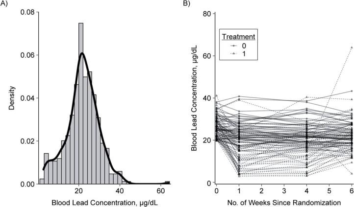
Distribution of blood lead concentrations (A) and change in blood lead concentrations over follow-up in the treated (treatment = 1) and placebo (treatment = 0) groups (B), among 100 participants in the Treatment of Lead-Exposed Children (TLC) Trial, United States, 1994–1997.

Notably, the intracluster correlation coefficient in these data is 0.6, suggesting an important degree of correlation for the outcome of interest.

IGNORING CORRELATED OUTCOMES

Ignoring correlations, we fitted a linear regression model to the data by regressing blood lead concentrations against the treatment. We obtained a mean difference of −5.6 μg/dL comparing the succimer-treated to the placebo group. The model-based standard error for this estimate is 0.75, which results in a 95% normal-interval (Wald) confidence interval for the mean difference of −7.1, −4.1. This analysis also assumes that each of the 400 observations in the data are independent. However, the intracluster correlation coefficient suggests otherwise, implying that the standard error for the mean difference quantified above is smaller than it should be.

ROBUST STANDARD ERRORS

One simple way to account for clustering is to use robust standard errors. Heteroscedastic-consistent (HC) robust standard errors can be used when the conditional variance of the outcome is not constant across all observations, by relying on the individual-level residuals from the model to adjust the standard error appropriately. A classic example of this involves the relationship between diet and income. As income increases, the variability in food consumption tends also to increase (4). Assuming constant variance (which one does when using model-based standard errors) would not be valid and could lead to misleading inferences. A large number of heteroscedasticity-consistent (HC) variance estimators exist (e.g., HC1, HC2, HC3, as described in Mansournia et al. (5)).

The cluster robust variance estimator modifies the HC variance estimator by relying on the individual-level residuals from the model, summed within each cluster, to adjust the standard error appropriately. In implementing the cluster robust HC3 variance estimator, we obtain, as expected, the same mean difference but a standard error of 1.1, yielding a larger 95% confidence interval of −7.8, −3.4.

CLUSTERED BOOTSTRAP

Alternatively, we could use a version of the nonparametric bootstrap that accounts for clustered outcomes. The nonparametric bootstrap requires appropriately resampling the data with replacement, and obtaining a set of point estimates from these resamples. Several variations of the bootstrap exist, including the normal-interval (i.e., Wald), percentile, bias-corrected, and bias-corrected and accelerated (6). These differ on the basis of the information they use in the point estimates obtained from the resamples. The normal-interval bootstrap is the simplest to use, and proceeds by using the standard deviation of all point estimates obtained from the resamples as a standard error in the Wald equation.

The clustered normal-interval bootstrap is identical to the standard normal-interval bootstrap except that instead of resampling observations, the clustered units are collectively resampled with replacement. By resampling this way, the “within-cluster” correlation structure is maintained, enabling us to obtain standard errors that appropriately account for clustering. After implementing the clustered bootstrap, we obtain the same mean difference, a standard error of 1.1, with a 95% confidence interval of −7.7, −3.5.

While we do not present results from a GEE or mixed model analysis here, our GitHub repository includes R (R Foundation for Statistical Computing) code and comments that elaborate on when all 4 methods are identical and when they differ, and that demonstrates both the additional work required and information obtained from GEE and mixed effects models.

Clearly, when using the robust variance estimator or bootstrap, we are only adjusting the standard errors to account for the fact that the outcomes are correlated. Both the robust variance estimator and the clustered bootstrap treat the clustering as a nuisance that is not of substantive interest. If researchers are interested in how the outcomes are correlated within clusters, these methods will not easily provide such information.

The robust variance estimator and the bootstrap are both subject to important limitations. The most important threat to the validity of the robust variance estimator is small sample sizes. Small sample adjustments exist, but (in contrast to Stata (StataCorp LLC, College Station, Texas)) are not the default in R. They are, however, easily implemented in R (7). Unfortunately, even with a small sample adjustment, there is a limit to how small the number of clusters can be. While dependent upon numerous aspects of the data (e.g., correlations between covariates, skewness of covariates), caution is warranted when fewer than 30 clusters are available.

For the clustered bootstrap, there is often a misconception that it does not require large samples to be valid. While there is simulation evidence showing that the performance of the bootstrap is better than the robust variance estimator in smaller sample sizes (8), the theoretical validity of the bootstrap still rests on large-sample (i.e., asymptotic) arguments. Nevertheless, in applied settings with fewer than 50 clusters, the clustered bootstrap may be a useful alternative to the robust variance estimator.

REFERENCES

- 1. Cole SR, Chu H, Greenland S. Maximum likelihood, profile likelihood, and penalized likelihood: a primer. Am J Epidemiol. 2013;179(2):252–260. [DOI] [PMC free article] [PubMed] [Google Scholar]
- 2. Zorn CJW. Generalized estimating equation models for correlated data: a review with applications. Am J Polit Sci. 2001;45(2):470–490. [Google Scholar]
- 3. Fitzmaurice GM, Laird NM, Ware JH. Applied Longitudinal Analysis. Hoboken, NJ: Wiley-Interscience; 2004. [Google Scholar]
- 4. Hill RC, Griffiths WE, Lim GC. Principles of Econometrics. 5th ed. Hoboken, NJ: John Wiley & Sons; 2018. [Google Scholar]
- 5. Mansournia MA, Nazemipour M, Naimi AI, et al. Reflection on modern methods: demystifying robust standard errors for epidemiologists. Int J Epidemiol. 2021;50(1):346–351. [DOI] [PubMed] [Google Scholar]
- 6. Efron B, Tibshirani R. Introduction to the Bootstrap. Boca Raton, FL: Chapman & Hall/CRC; 1993. [Google Scholar]
- 7. Zeileis A, Köll S, Graham N. Various versatile variances: an object-oriented implementation of clustered Covariances in R. J Stat Softw. 2020;95(1):1–36. [Google Scholar]
- 8. Cameron AC, Gelbach JB, Miller DL. Bootstrap-based improvements for inference with clustered errors. Rev Econ Stat. 2008;90(3):414–427. [Google Scholar]