Abstract
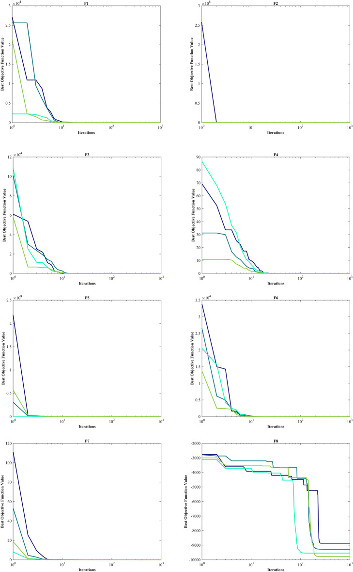
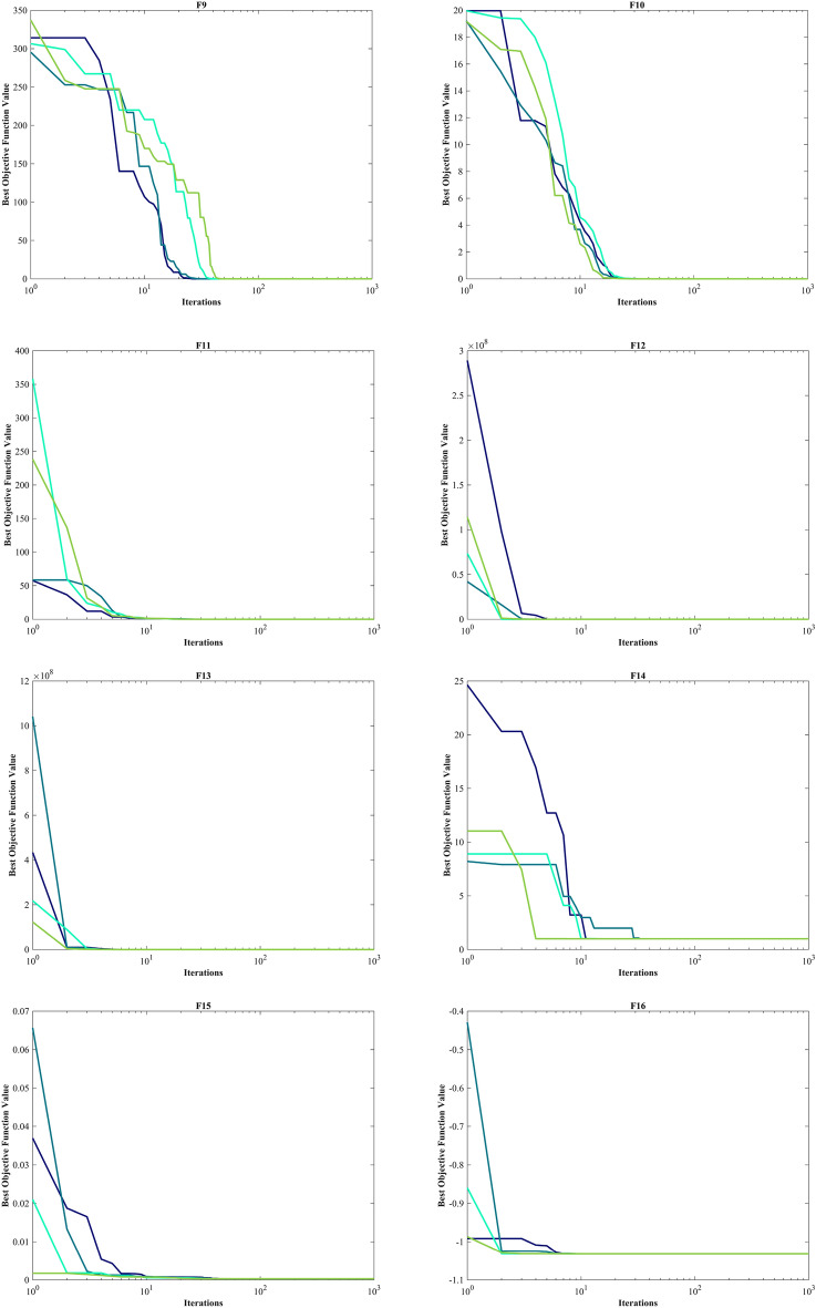
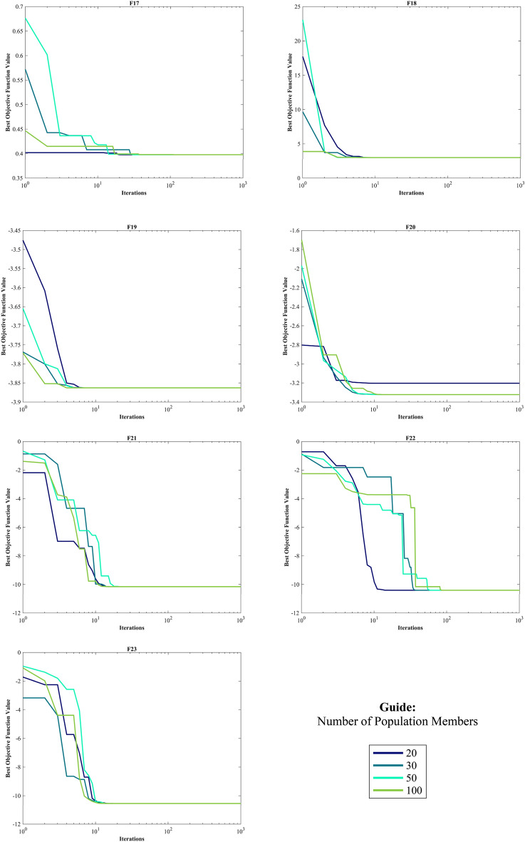
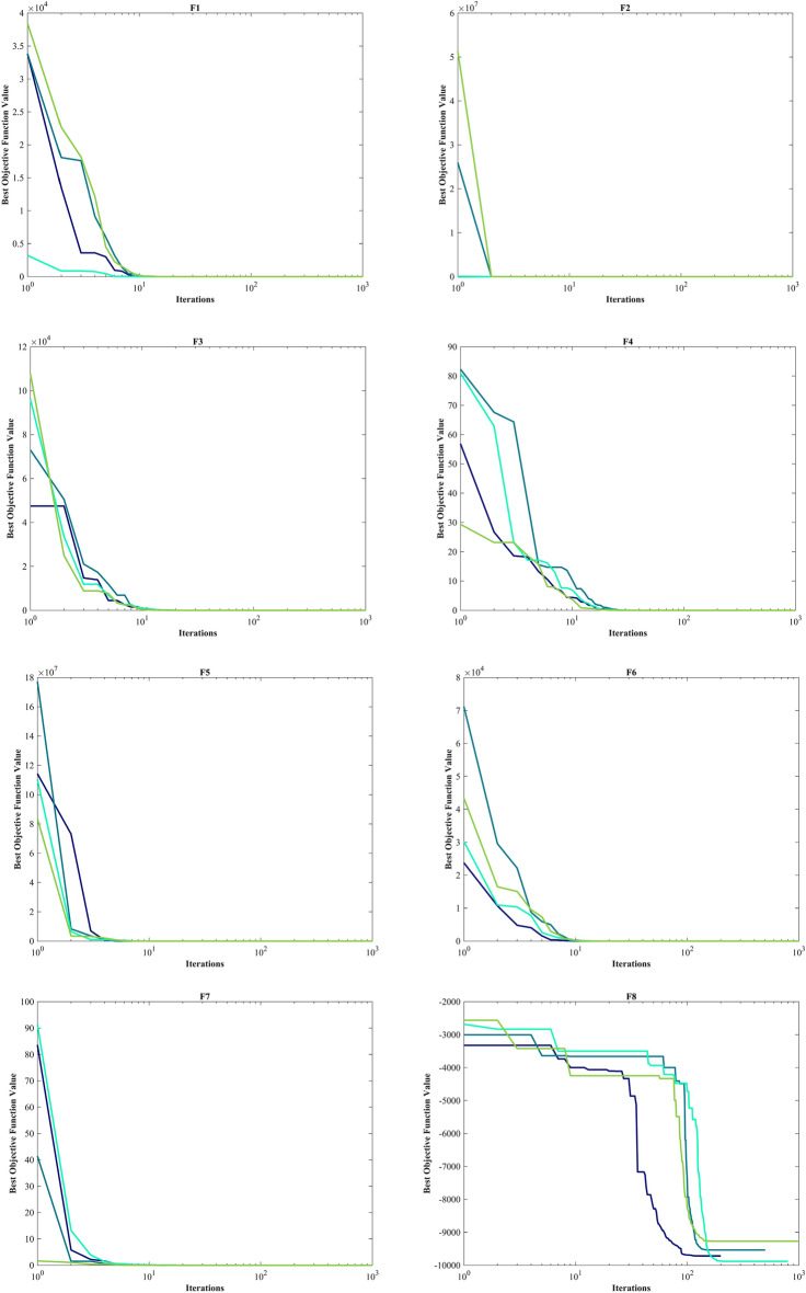
The novelty of this article lies in introducing a novel stochastic technique named the Hippopotamus Optimization (HO) algorithm. The HO is conceived by drawing inspiration from the inherent behaviors observed in hippopotamuses, showcasing an innovative approach in metaheuristic methodology. The HO is conceptually defined using a trinary-phase model that incorporates their position updating in rivers or ponds, defensive strategies against predators, and evasion methods, which are mathematically formulated. It attained the top rank in 115 out of 161 benchmark functions in finding optimal value, encompassing unimodal and high-dimensional multimodal functions, fixed-dimensional multimodal functions, as well as the CEC 2019 test suite and CEC 2014 test suite dimensions of 10, 30, 50, and 100 and Zigzag Pattern benchmark functions, this suggests that the HO demonstrates a noteworthy proficiency in both exploitation and exploration. Moreover, it effectively balances exploration and exploitation, supporting the search process. In light of the results from addressing four distinct engineering design challenges, the HO has effectively achieved the most efficient resolution while concurrently upholding adherence to the designated constraints. The performance evaluation of the HO algorithm encompasses various aspects, including a comparison with WOA, GWO, SSA, PSO, SCA, FA, GOA, TLBO, MFO, and IWO recognized as the most extensively researched metaheuristics, AOA as recently developed algorithms, and CMA-ES as high-performance optimizers acknowledged for their success in the IEEE CEC competition. According to the statistical post hoc analysis, the HO algorithm is determined to be significantly superior to the investigated algorithms. The source codes of the HO algorithm are publicly available at https://www.mathworks.com/matlabcentral/fileexchange/160088-hippopotamus-optimization-algorithm-ho.
Subject terms: Engineering, Mathematics and computing
Introduction
Numerous issues and challenges in today's science, industry, and technology can be defined as optimization problems. All optimization problems have three parts: an objective function, constraints, and decision variables1. Optimization algorithms can be categorized in diverse manners for addressing such problems. Nonetheless, one prevalent classification method is based on its inherent approach to optimizing problems, distinguishing between stochastic and deterministic algorithms2. Unlike stochastic methods, deterministic methods require more extensive information about the problem3. However, stochastic methods do not guarantee finding a global optimal solution. In today's context, optimization problems we often encounter are nonlinear, complex, non-differentiable, piecewise functions, non-convex, and involve many decision variables4. For such problems, employing stochastic methods for their solution tends to be more straightforward and more suitable, especially when we have limited information about the problem or intend to treat it as a black box5.
One of the most important and widely used methods in stochastic approaches is metaheuristic algorithms. In metaheuristic algorithms, feasible initial solution candidates are randomly generated. Then, iteratively, these initial solutions are updated according to the specified relationships in the metaheuristic algorithm. In each step, feasible solutions with better costs are retained based on the number of search agents. This updating continues until the stopping iteration is satisfied, typically achieving a MaxIter such as the Number of Function Evaluations (NFE) or reaching a predefined cost value set by the user for the cost function. Because of the advantages of metaheuristic algorithms, they are used in various applications, and the results show that these algorithms can improve efficiency in these applications. A good optimization algorithm is able to create a balance between exploration and exploitation, in the sense that in exploration, attention is paid to global search, and in exploitation, attention is paid to local search around the obtained answers6.
Numerous optimization algorithms have been introduced; however, introducing and developing a new, highly innovative algorithm are still deemed necessary, as per the No Free Lunch (NFL) theorem7. The NFL theorem asserts that the superior performance of a metaheuristic algorithm in solving specific optimization problems does not guarantee similar success in solving different problems. Therefore, the need for an algorithm that demonstrates improved speed of convergence and the ability to find the optimal solution compared to other algorithms is highlighted. The broad scope of utilizing metaheuristic optimization algorithms has garnered attention from researchers across multiple disciplines and domains. Metaheuristic optimization algorithms find applications in a wide range of engineering disciplines, including medical engineering problems, such as improving classification accuracy by adjusting hyperparameters using metaheuristic optimization algorithms and adjusting weights in neural networks8 or fuzzy systems9.
Similarly, these algorithms contribute to intelligent fault diagnosis and tuning controller coefficients10 in control and mechanical engineering. In telecommunication engineering, they aid in identifying digital filters11, while in energy engineering, they assist in tasks such as modeling solar panels12, optimizing their placement, and even wind turbine placement13. In civil engineering, metaheuristic optimization algorithms are utilized for structural optimization14, while in the field of economics, they enhance stock portfolio optimization15. Additionally, metaheuristic optimization algorithms play a role in optimizing thermal systems in chemical engineering16, among other applications.
The distinctive contributions of this research lie in developing a novel metaheuristic algorithm termed the HO, rooted in the emulation of Hippopotamuses' behaviors in the natural environment. The primary achievements of this study work can be outlined as follows:
The design of HO is influenced by the intrinsic behaviors observed in hippopotamuses, such as their position update in the river or pond, defence tactics against predators, and methods of evading predators.
HO is mathematically formulated through a three-phase model comprising their position update, defence, and evading predators.
To evaluate the effectiveness of the HO in solving optimization problems, it undergoes testing on a set of 161 standard BFs of various types of UM, MM, ZP benchmark test, the CEC 2019, the CEC 2014 dimensions of 10, 30, 50, and 100 to investigate the effect of the dimensions of the problem on the performance of the HO algorithm
The performance of the HO is evaluated by comparing it with the performance of twelve widely well-kown metaheuristic algorithms.
The effectiveness of the HO in real-world applications is tested through its application to tackle four engineering design challenges.
The article is structured into five sections. The “Literature review’’ section focuses on related work, while the “Hippopotamus Optimization Algorithm” section covers the HO approach introduced, modelled, and HO's limitations. The “Simulation results and comparison” section presents simulation results and compares the performance of the different algorithms. The performance of HO in solving classical engineering problems is studied in the “Hippopotamus optimization algorithm for engineering problems” section, and “Conclusions and future works” section provides conclusions based on the article's findings.
Literature review
As mentioned in the introduction, it should be noted that optimization algorithms are not confined to a singular discipline or specialized research area. This is primarily because numerous real-world problems possess intricate attributes, including nonlinearity, non-differentiability, discontinuity, and non-convexity. Given these complexities and uncertainties, stochastic optimization algorithms demonstrate enhanced versatility and a heightened capacity to address such challenges effectively. Consequently, they exhibit a more remarkable ability to accommodate and navigate the intricacies and uncertainties inherent in these problems. Optimization algorithms often draw inspiration from natural phenomena, aiming to model and simulate natural processes. Physical laws, chemical reactions, animal behavior patterns, social behavior of animals, biological evolution, game theory principles, and human behavior have received significant attention in this regard. These natural phenomena serve as valuable sources of inspiration for developing optimization algorithms, offering insights into efficient and practical problem-solving strategies.
Optimization algorithms can be classified from multiple perspectives. In terms of objectives, they can be grouped into three categories: single-objective, multi-objective, and many-objective algorithms17. From the standpoint of decision variables, algorithms can be characterized as either continuous or discrete (or binary). Furthermore, they can be subdivided into constrained and unconstrained optimization algorithms, depending on whether constraints are imposed on the decision variables. Such classifications provide a framework for understanding and categorizing optimization algorithms based on different criteria. From another perspective, optimization algorithms can be categorized based on their sources of inspiration. These sources can be classified into six main categories: evolutionary algorithms, physics or chemistry-based algorithms, swarm-based algorithms, human-inspired algorithms, mathematic-based algorithms, and game theory-inspired algorithms. While the first four categories are well-established and widely recognized, the mathematic-based and game theory-inspired categories may need to be more known.
Optimization algorithms that draw inspiration from swarm-based are commonly utilized to model the collective behavior observed in animals, plants, and insects. For instance, the American Zebra Optimization Algorithm (ZOA)18. The inspiration for ZOA comes from the foraging behavior of zebras and their defensive behavior against predators during foraging. Similarly, the inspiration for Northern Goshawk Optimization (NGO)19 comes from the hunting behavior of the Northern Goshawk. Among the notable algorithms in this category are Particle Swarm Optimization (PSO)20, Ant Colony Optimization (ACO)21, and Artificial Bee Colony (ABC) algorithm22, Tunicate Swarm Algorithm (TSA)23, Beluga Whale Optimization (BWO)24, Aphid–Ant Mutualism (AAM)25, artificial Jellyfish Search (JS)26, Spotted Hyena Optimizer (SHO)27, Honey Badger Algorithm (HBA)28, Mantis Search Algorithm (MSA)29, Nutcraker Optimization Algorithm (NOA)30, Manta Ray Foraging Optimization (MRFO)31, Orca Predation Algorithm (OPA)32, Yellow Saddle Goatfish (YSG)33, Hermit Crab Optimization Algorithm (HCOA)34, Cheetah Optimizer (CO)35, Walrus Optimization Algorithm (WaOA)36, Red-Tailed Hawk algorithm (RTH)37, Barnacles Mating Optimizer (BMO)38, Meerkat Optimization Algorithm (MOA)39, Snake Optimizer (SO)40, Grasshopper Optimization Algorithm (GOA)41, Social Spider Optimization (SSO)42, Whale Optimization Algorithm (WOA)43, Ant Lion Optimizer (ALO)44, Grey Wolf Optimizer (GWO)45, Marine Predators Algorithm (MPA)46 ,Aquila Optimizer (AO)47, Mountain Gazelle Optimizer (MGO)48, Artificial Hummingbird Algorithm (AHA)49, African Vultures Optimization Algorithm (AVOA)50, Bonobo Optimizer (BO)51, Salp Swarm Algorithm (SSA)52, Harris Hawks Optimizer (HHO)53, Colony Predation Algorithm (CPA)54, Adaptive Fox Optimization (AFO)55, Slime Mould Algorithm (SMA)3, Spider Wasp Optimization (SWO)56, Artificial Gorilla Troops Optimizer (GTO)57, Krill Herd Optimization (KH)58, Alpine Skiing Optimization (ASO)59, Shuffled Frog-Leaping Algorithm (SFLA)60, Firefly Algorithms (FA)61, Komodo Mlipir Algorithm (KMA)62, Prairie Dog Optimization (PDO)63, Tasmanian Devil Optimization (TDO)64, Reptile Search Algorithm (RSA)65, Border Collie Optimization (BCO)66, Cuckoo Optimization Algorithm (COA)67 and Moth-flame optimization algorithm (MFO)68 are novel optimization algorithm that has been introduced in recent years. They belong to the category of swarm-based optimization algorithms. These algorithms encapsulate the principles of swarm intelligence, offering effective strategies for solving optimization problems by emulating the cooperative and adaptive behaviors found in natural swarms.
Another category of optimization algorithms is based on the origin of inspiration from biological evolution, genetics, and natural selection. The genetic optimization algorithm (GA)69 is one of the most well-known algorithms in this category. Among the notable algorithms in this category are Memetic Algorithm (MA)70, Differential Evolution (DE)71 Evolution Strategies (ES)72 Biogeography-Based Optimization (BBO)73, Liver Cancer Algorithm (LCA)74, Genetic Programming (GP)75, Invasive Weed Optimization algorithm (IWO)76, Electric Eel Foraging Optimization (EEFO)77, Greylag Goose Optimization (GGO)78 , and Puma Optimizer (PO)79. The Competitive Swarm Optimizer (CSO)80 is crafted explicitly for handling large-scale optimization challenges, taking inspiration from PSO while introducing a unique conceptual approach. In CSO, the adjustment of particle positions deviates from the inclusion of personal best positions or global best positions. Instead, it employs a pairwise competition mechanism, allowing the losing particle to learn from the winner and adjust its position accordingly. The Falcon Optimization Algorithm (FOA)81 is inspired by the hunting behavior of falcons. The Barnacles Mating Optimizer (BMO)82 algorithm takes inspiration from the mating behavior observed in barnacles in their natural habitat. The Pathfinder Algorithm (PFA)83 is tailored to address optimization problems with diverse structures. Drawing inspiration from the collective movement observed in animal groups and the hierarchical leadership within swarms, PFA seeks to discover optimal solutions akin to identifying food areas or prey.
Optimization algorithms are based on the origin of physical or chemical laws. As the name of this category suggests, the concepts are inspired by physical laws, chemical reactions, or chemical laws. Some of the algorithms in this category include Simulated Annealing (SA)84, Snow Ablation Optimizer (SAO)85, Electromagnetic Field Optimization (EFO)86, Light Spectrum Optimization (LSO)87, String Theory Algorithm (STA)88, Harmony Search (HS)89, Multi-Verse Optimizer (MVO)90, Black Hole Algorithm (BH)91, Gravitational Search Algorithm (GSA)92, Artificial Electric Field Algorithm (AEFA)93 draws inspiration from the principles of Coulomb's law governing electrostatic force. Magnetic Optimization Algorithm (MOA)94, Chemical Reaction Optimization (CRO)95 , Atom Search Optimization (ASO)96, Henry Gas Solubility Optimization (HGSO)97, Nuclear Reaction Optimization (NRO)98, Chernobyl Disaster Optimizer (CDO)99, Thermal Exchange Optimization (TEO)100, Turbulent Flow of Water-based Optimization (TFWO)101, Water Cycle Algorithm (WCA)102, Equilibrium Optimizer (EO)103, Lévy Flight Distribution (LFD)104, and Crystal Structure Algorithm (CryStAl)105 which takes inspiration from the symmetric arrangement of constituents in crystalline minerals like quartz.
Human-inspired algorithms derive inspiration from the social behavior, learning processes, and communication patterns found within human society. Some of the algorithms in this category include Driving Training-Based Optimization (DTBO)106, Fans Optimization (FO)107, Mother Optimization Algorithm (MOA)108, Mountaineering Team-Based Optimization (MTBO)109, Human Behavior-Based Optimization (HBBO)110, Chef-Based Optimization Algorithm (CBOA)111 is the process of acquiring culinary expertise through training programs. Teaching–Learning-Based Optimization (TLBO)112, Political Optimizer (PO)113, In the War Strategy Optimization (WSO)114 optimization algorithm, two human strategies during war, attack and defence, are modelled. EVolutive Election Based Optimization (EVEBO)115, Distance-Fitness Learning (DFL)116, and Cultural Algorithms (CA)117. Supply–Demand-Based Optimization (SDO)118 is inspired by the economic supply–demand mechanism and is crafted to emulate the dynamic interplay between consumers' demand and producers' supply. The Search and Rescue Optimization Algorithm (SAR)119 takes inspiration from the exploration behavior observed during search and rescue operations conducted by humans. The Student Psychology Based Optimization (SPBO)120 algorithm draws inspiration from the psychology of students who aim to enhance their exam performance and achieve the top position in their class. The Poor and Rich Optimization (PRO)121 algorithm is inspired by the dynamics between the efforts of poor and rich individuals to improve their economic situations. The algorithm mirrors the behavior of both the rich, who seek to widen the wealth gap, and the poor, who endeavor to accumulate wealth and narrow the gap with the affluent.
Game-based optimization algorithms often model the rules of a game. Some of the algorithms in this category include Squid Game Optimizer (SGO)122, Puzzle Optimization Algorithm (POA)123, and Darts Game Optimizer (DGO)124.
Mathematical theories inspire mathematical algorithms. For example, Arithmetic Optimization Algorithm (AOA)125 ,the Chaos Game Optimization (CGO)126 is inspired by chaos theory and fractal configuration principles. Another known algorithm in this category are Sine Cosine Algorithm (SCA)127, Evolution Strategy with Covariance Matrix Adaptation (CMA-ES)128, and Quadratic Interpolation Optimization (QIO).
Hippopotamus optimization algorithm
In this section, we articulate the foundational inspiration and theoretical underpinnings of the proposed HO Algorithm.
Hippopotamus
The hippopotamus is one of the fascinating creatures residing in Africa129. This animal falls under the classification of vertebrates and specifically belongs to the group of mammals within the vertebrate category130. Hippopotamuses are semi-aquatic organisms that predominantly occupy their time in aquatic environments, specifically rivers and ponds, as part of their habitat131,132. Hippopotamuses exhibit a social behavior wherein they reside in collective units referred to as pods or bloats, typically comprising a population ranging from 10 to 30 individuals133. Determining the gender of hippopotamuses is not easily accomplished as their sexual organs are not external, and the only distinguishing factor lies in the difference in their weight. Adult hippopotamuses can stay submerged underwater for up to 5 min. This species of animal, in terms of appearance, bears resemblance to venomous mammals such as the shrew, but its closest relatives are whales and dolphins, with whom they shared a common ancestor around 55 million years ago134.
Despite their herbivorous nature and reliance on a diet consisting mainly of grass, branches, leaves, reeds, flowers, stems, and plant husks135, hippopotamuses display inquisitiveness and actively explore alternative food sources. Biologists believe that consuming meat can cause digestive issues in hippopotamuses. These animals possess extremely powerful jaws, aggressive temperament, and territorial behavior, which has classified them as one of the most dangerous mammals in the world136. The weight of male hippopotamuses can reach up to 9,920 pounds, while females typically weigh around 3,000 pounds. They consume approximately 75 pounds of food daily. Hippopotamuses engage in frequent conflicts with one another, and occasionally, during these confrontations, one or multiple hippopotamus calves may sustain injuries or even perish. Due to their large size and formidable strength, predators generally do not attempt to hunt or attack adult hippopotamuses. However, young hippopotamuses or weakened adult individuals become vulnerable prey for Nile crocodiles, lions, and spotted hyenas134.
When attacked by predators, hippopotamuses exhibit a defensive behavior by rotating towards the assailant and opening their powerful jaws. This is accompanied by emitting a loud vocalization, reaching approximately 115 decibels, which instils fear and intimidation in the predator, often deterring them from pursuing such a risky prey. When the defensive approach of a hippopotamus proves ineffective or when the hippopotamus is not yet sufficiently strong, it retreats rapidly at speeds of approximately 30 km/h to distance itself from the threat. In most cases, it moves towards nearby water bodies such as ponds or rivers136.
Inspiration
The HO draws inspiration from three prominent behavioral patterns observed in the life of hippopotamuses. Hippopotamus groups are comprised of several female hippopotamuses, hippopotamus calves, multiple adult male hippopotamuses, and a dominant male hippopotamus (the leader of the herd)136. Due to their inherent curiosity, young and calves hippopotamuses often display a tendency to wander away from the group. As a consequence, they may become isolated and become targets for predators.
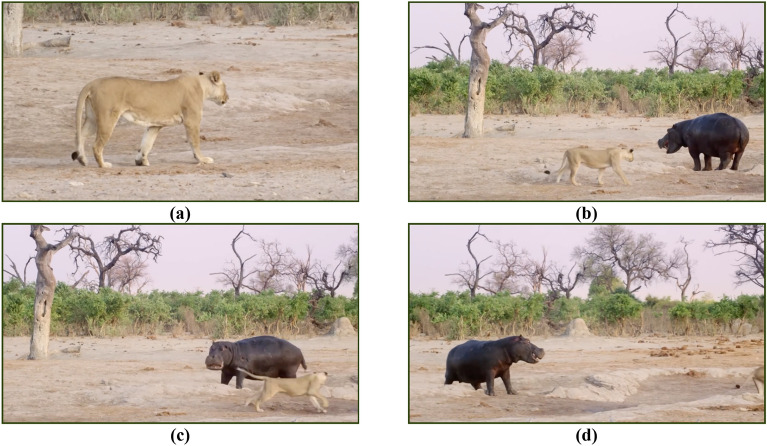
The secondary behavioral pattern of hippopotamuses is defensive in nature, triggered when they are under attack by predators or when other creatures intrude into their territory. Hippopotamuses exhibit a defensive response by rotating themselves toward the predator and employing their formidable jaws and vocalizations to deter and repel the attacker (Fig. 1). Predators such as lions and spotted hyenas possess an awareness of this phenomenon and actively seek to avoid direct exposure to the formidable jaws of a hippopotamus as a precautionary measure against potential injuries. The final behavioral pattern encompasses the hippopotamus' instinctual response of fleeing from predators and actively seeking to distance itself from areas of potential danger. In such circumstances, the hippopotamus strives to navigate toward the closest body of water, such as a river or pond, as lions and spotted hyenas frequently exhibit aversion to entering aquatic environments.
Figure 1.
(a–d) shows the defensive behavior of the hippopotamus against the predator136.
Mathematical modelling of HO
The HO is a population-based optimization algorithm, in which search agents are hippopotamuses. In the HO algorithm, hippopotamuses are candidate solutions for the optimization problem, meaning that the position update of each hippopotamus in the search space represents values for the decision variables. Thus, each hippopotamus is represented as a vector, and the population of hippopotamuses is mathematically characterized by a matrix. Similar to conventional optimization algorithms, the initialization stage of the HO involves the generation of randomized initial solutions. During this step, the vector of decision variables is generated using the following formula:
| 1 |
where represents the position of the th candidate solution, is a random number in the range of 0 to 1, and and denote the lower and upper bounds of the th decision variable, respectively. Given that denotes the population size of hippopotamuses within the herd, and m represents the number of decision variables in the problem, the population matrix is formed by Eq. (2).
| 2 |
Phase 1: The hippopotamuses position update in the river or pond (Exploration)
Hippopotamus herds are composed of several adult female hippopotamuses, calves hippopotamuses, multiple adult male hippopotamuses, and dominant male hippopotamuses (the leader of the herd). The dominant hippopotamus is determined based on the objective function value iteration (The lowest for the minimization problem and the highest for the maximization problem). Typically, hippopotamuses tend to gather in close proximity to one another. Dominant male hippopotamuses protect the herd and territory from potential threats. Multiple female hippopotamuses are positioned around the male hippopotamuses. Upon reaching maturity, male hippopotamuses are ousted from the herd by the dominant male. Subsequently, these expelled male individuals are required to either attract females or engage in dominance contests with other established male members of the herd in order to establish their own dominance. Equation (3) expresses the mathematical representation of the position of male hippopotamus members of the herd in the lake or pond.
| 3 |
In Eq. (3) represents male hippopotamus position, denotes the dominant hippopotamus position (The hippopotamus that has the best cost in the current iteration). is a random vector between 0 and 1, is a random number between 0 and 1 (Eq. 4), and is an integer between 1 and 2 (Eqs. 3 and 6). refers to the mean values of some randomly selected hippopotamus with an equal probability of including the current considered hippopotamus () and is a random number between 0 and 1 (Eq. 3). In Eq. (4) and are integer random numbers that can be one or zero.
| 4 |
| 5 |
| 6 |
| 7 |
Equations (6) and (7) describe female or immature hippopotamus position () within the herd. Most immature hippopotamuses are near their mothers, but due to curiosity, sometimes immature hippopotamuses are separated from the herd or away from their mothers. If is greater than 0.6, it means the immature hippopotamus has distanced itself from its mother (Eq. 5). If , which is a number between 0 and 1 (Eq. 7), is greater than 0.5, it means the immature hippopotamus has distanced itself from its mother but is still within or near the herd, Otherwise, it has separated from the herd. This behavior of immature and female hippopotamuses is modelled according to Eqs. (6) and (7). and are numbers or vectors randomly selected from the five scenarios in the equation. In Eq. (7) is a random number between zero and one. Equations (8), (9) describe male and female or immature hippopotamus position update within the herd. is objective function value.
| 8 |
| 9 |
Using vectors, and scenarios enhance the global search and improves exploration in the proposed algorithm. It leads to a better global search and enhances the exploration process in the proposed algorithm.
Phase 2: Hippopotamus defence against predators (Exploration)
One of the key reasons for the herd living of hippopotamuses can be attributed to their safety and security. The presence of these large and heavy-weighted herding’s of animals can deter predators from approaching them closely. Nevertheless, due to their inherent curiosity, immature hippopotamuses may occasionally deviate from the herd and become potential targets for Nile crocodiles, lions, and spotted hyenas, given their relatively lesser strength in comparison to adult hippopotamuses. Sick hippopotamuses, similar to immature ones, are also susceptible to being preyed upon by predators.
The primary defensive tactic employed by hippopotamuses is swiftly turning towards the predator and emitting loud vocalizations to deter the predator from approaching them closely (Fig. 2). During this phase, hippopotamuses may exhibit a behavior of approaching the predator to induce its retreat, thus effectively warding off the potential threat. Equation (10) represents the predator's position in search space.
| 10 |
where represents a random vector ranging from zero to one.
| 11 |
Figure 2.
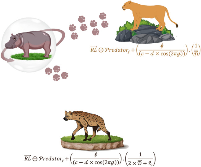
Graphic representation of the phase 2.
Equation (11) indicates the distance of the hippopotamus to the predator. During this time, the hippopotamus adopts a defensive behavior based on the factor to protect itself against the predator. If is less than , indicating the predator is in very close proximity to the hippopotamus, in such a case, the hippopotamus swiftly turns towards the predator and moves towards it to make it retreat. If is greater, it indicates that the predator or intruding entity is at a greater distance from the hippopotamus's territory Eq. (12). In this case, the hippopotamus turns towards the predator but with a more limited range of movement. The intention is to make the predator or intruder aware of its presence within its territory.
| 12 |
is a hippopotamus position which was faced to predator. is a random vector with a Levy distribution, utilized for sudden changes in the predator's position during an attack on the hippopotamus. The mathematical model for the random movement of Lévy movement46 is calculated as Eq. (13). and are the random numbers in [0,1], respectively; is a constant ( = 1.5), is an abbreviation for Gamma function and can be obtained by Eq. (14).
| 13 |
| 14 |
In Eq. (12) is a uniform random number between 2 and 4, is a uniform random number between 1 and 1.5 and is a uniform random number between 2 and 3. represents a uniform random number between − 1 and 1. is a random vector with dimensions .
According to the Eq. (15), if is greater than , it means that the hippopotamus has been hunted and another hippopotamus will replace it in the herd, otherwise the hunter will escape and this hippopotamus will return to the herd. Significant enhancements were observed in the global search process during the second phase. The first and second phases complement each other and effectively mitigate the risk of getting trapped in local minima.
| 15 |
Phase 3: Hippopotamus Escaping from the Predator (Exploitation)
Another behavior of a hippopotamus in the face of a predator is when the hippopotamus encounters a group of predators or is unable to repel the predator with its defensive behavior. In this situation, the hippopotamus tries to move away from the area (Fig. 3). Usually, the hippopotamus tries to run to the nearest lake or pond to avoid the harm of predators because spotted lions and hyenas avoid entering the lake or pond. This strategy leads to the hippopotamus finding a safe position close to its current location and modelling this behavior in Phase Three of the HO results in an enhanced ability for exploitation in local search. To simulate this behavior, a random position is generated near the current location of the hippopotamuses. This behavior of the hippopotamuses is modelled according to Eqs. (16–19). When the newly created position improves the cost function value, it indicates that the hippopotamus has found a safer position near its current location and has changed its position accordingly. denotes the current iteration, while represents the MaxIter.
| 16 |
| 17 |
Figure 3.
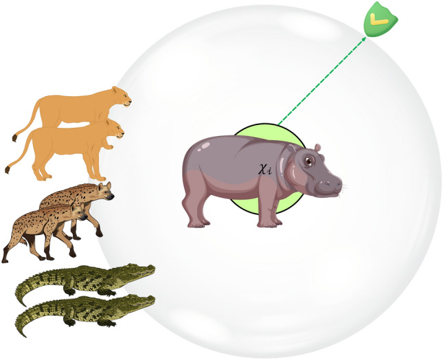
Drawing a Hippopotamus Escaping from the Predator.
In Eq. (17), is the position of hippopotamus which was searched to find the closest safe place. is a random vector or number that is randomly selected from among three scenarios Eq. (18). The considered scenarios () lead to a more suitable local search or, in other words, result in the proposed algorithm having a higher exploitation quality.
| 18 |
In Eq. (18) represents a random vector between 0 and 1, while (Eq. 17) and denote random numbers generated within the range of 0 and 1. Additionally, is a normally distributed random number.
| 19 |
In the HO algorithm to update the population, we did not divide the population into three separate categories of immature, female, and male hippopotamus because although dividing them into separate categories would be better modelling of their nature, it would reduce the performance of the optimization algorithm.
Repetition process, and flowchart of HO
After completing each iteration of the HO algorithm, all population members are updated based on Phases 1 to 3 this process of updating the population according to Eqs. (3–19) continues until the final iteration.
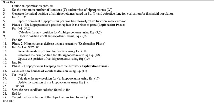
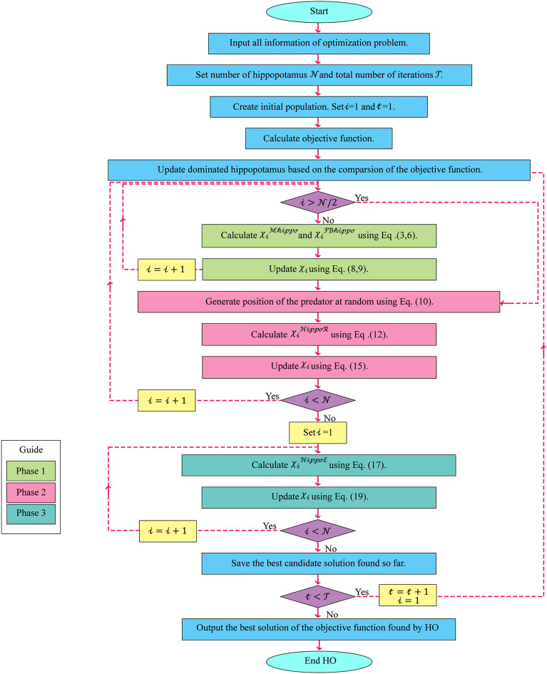
During the execution of the algorithm, the best potential solution is consistently tracked and stored. Upon the completion of the entire algorithm, the best candidate, referred to as the dominant hippopotamus solution, is unveiled as the ultimate solution to the problem. The HO's procedural details are shown in Fig. 4 flowchart and Algorithm 1's pseudocode.
Algorithm 1.
Pseudo-code of HO.
Figure 4.
HO's flowchart.
Computational complexity of HO
In this subsection, the HO computational complexity analysis is discussed. The total computational complexity of HO is equal to The represents the computational complexity of the initial assignment of the algorithm, which is the same for all metaheuristic optimization algorithms. The computational complexity of the initial phase in HO is denoted as . The computational complexity of the second phase in HO is . Finally, the computational complexity of the third phase is . Therefore, the total computational complexity of the main loop is
Regarding competitor algorithms, WOA, GWO, SSA, PSO, SCA, FA, GOA, CMA-ES, SSA, MFO, and IWO have a time complexity equal to and TLBO and AOA have a computational complexity equal to Nevertheless, in order to ensure equitable comparative analysis, we standardized the population size for each algorithm within the simulation study, thereby ensuring uniformity in the total count of function evaluations across all algorithms utilized. Other algorithms with higher time complexity were introduced, for instance, CGO, which exhibits a computational complexity of .
Limitation of HO
The initial constraint of the HO, akin to all metaheuristic algorithms, lies in the absence of assurance regarding attaining the global optimum due to the stochastic search procedure. The second constraint stems from the NFL, implying the perpetual potential for newer metaheuristic algorithms to outperform HO. A further constraint involves the inability to assert HO as the preeminent optimizer across all optimization endeavors.
Simulation results and comparison
In this study, we juxtapose the efficacy of results attained through HO with a dozen established metaheuristic algorithms such as SCA, GWO, WOA, GOA, SSA, FA, TLBO, CMA-ES, IWO, MFO, AOA, and PSO. The adjustment of control parameters is detailed as per the specifications outlined in Table 1. This section presents simulation studies of the HO applied to various challenging optimization problems. The effectiveness of the HO in achieving optimal solutions is evaluated using a comprehensive set of 161 standard BFs. These functions encompass UM, high-dimensional, FM, and the CEC 2014, CEC 2019, ZP, and 4 engineering problems.
Table 1.
Assigned values to the control parameters of competitor algorithms.
| Algorithm | Parameter | Value |
|---|---|---|
| GWO | Convergence parameter () | Linear reduction from 2 to 0 |
| SCA | A | 2 |
| WOA | Convergence parameter () | Linear reduction 2 to 0 |
| Parameter | A random vector between 0 and 1 | |
| Parameter | A random vector between -1 and 1 | |
| PSO | Velocity limit | 10% of dimension range |
| Cognitive and social constant | ( | |
| Topology | Fully connected | |
| Inertia weight | Linear reduction from 0.9 to 0.1 | |
| GOA | 1.5 | |
| 0.5 | ||
| 0.00004 | ||
| 1 | ||
| SSA | Initial speed () | 0 |
| Leader position update probability | 0.5 | |
| FA | Alpha () | 0.2 |
| Beta () | 1 | |
| Gamma () | 1 | |
| TLBO | Teaching factor () | |
| A random number between 0 and 1 | ||
| CMA-ES | 0.5 | |
| AOA | 0 | |
| 0.5 | ||
| IWO | Minimum number of seeds () | 0 |
| Maximum number of seeds () | 5 | |
| Initial value of standard deviation | 1 | |
| Final value of standard deviation | 0.001 | |
| Variance reduction exponent | 2 | |
| MFO | b | 1 |
| r | Linear reduction -1 to -2 |
To enhance the performance of functions F1 to F2343, CEC 2019 test set, ZP, and engineering problems algorithms 30 independent runs encompassing 30,000 NFE and 60,000 NFE for CEC 2014 test set. The HO's population number is maintained at a constant of 24 members for AOA and TLBO set 30 and other algorithms is 60, and the MaxIter is set on 500 and 1000 (CEC 2014). A comprehensive set of six statistical metrics, namely mean, best, worst, Std., median, and rank, are utilized for presenting the optimization outcomes. The mean index is particularly employed as a pivotal ranking parameter for evaluating the efficacy of metaheuristic algorithms across each BF.
The specifications of the software and machines used for simulation are as follows; Core (TM) i3-1005G1 CPU processor with 1.20GHz with 8G for main memory and MacBook Air M1 with 8G for main memory.
Evaluation Unimodal benchmark functions
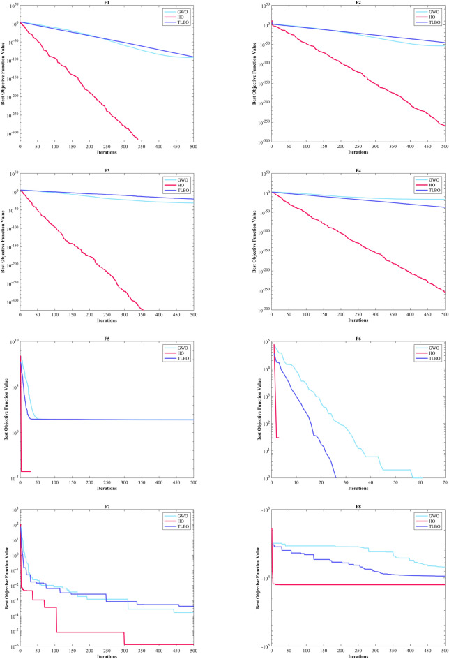
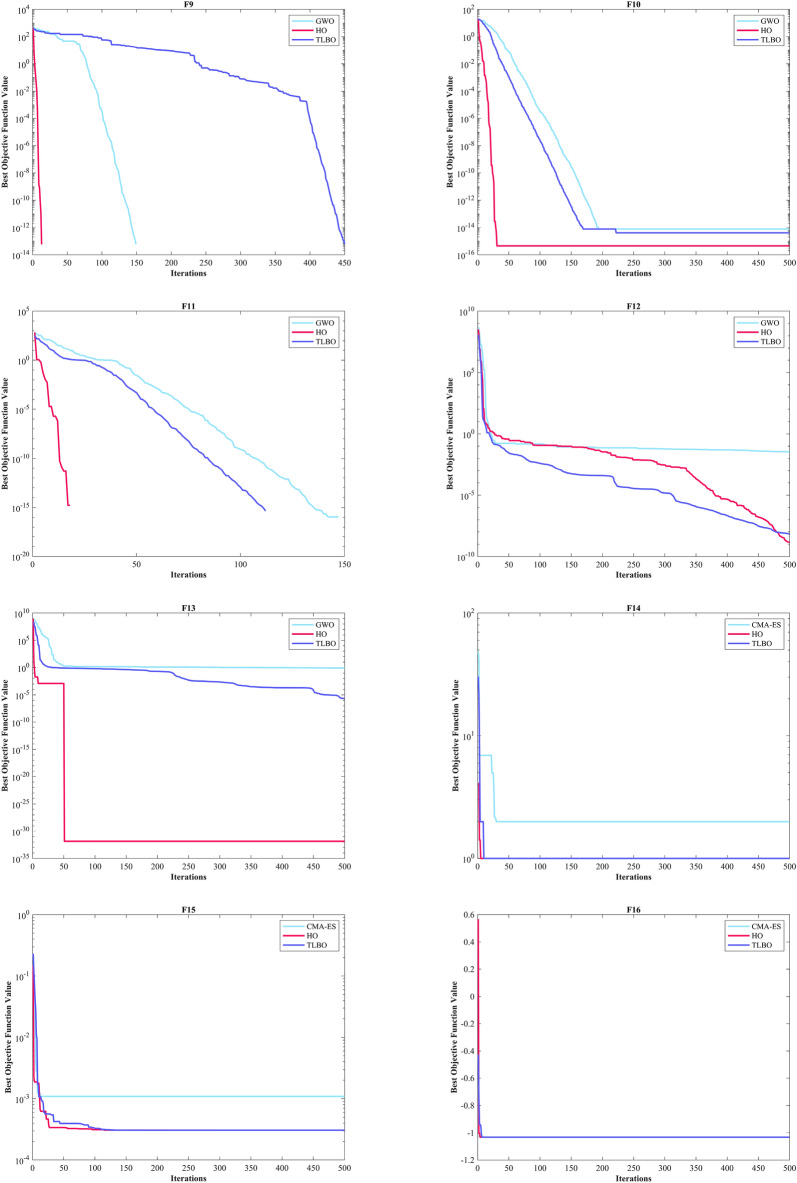
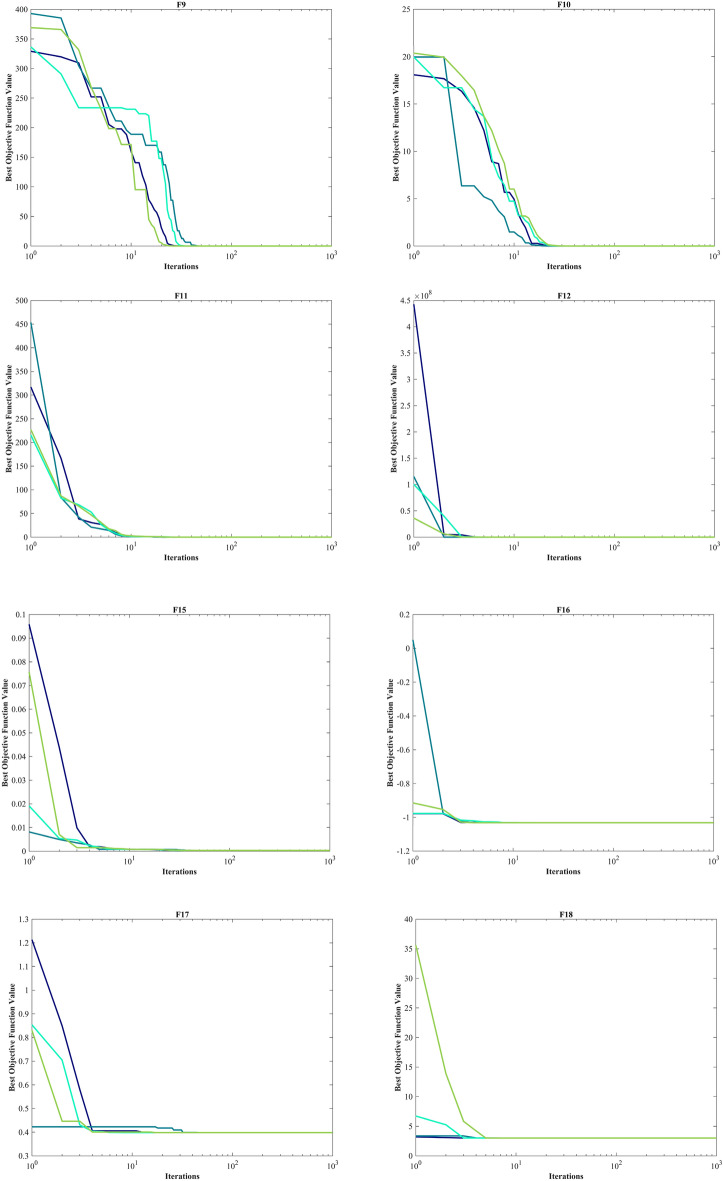
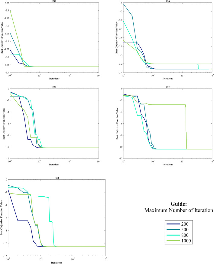
The assessment of functions was conducted, and the outcomes are presented in Table 2. Figure 6, shows convergence of the three most effective algorithms for optimizing F1-F23. This evaluation is to determine the ability of the algorithms to local search on seven separate UM functions, shown as F1-F7. The HO achieved global optimum for F1-F3 and F5-F6 a feat unattained by any of the 12 algorithms subjected to evaluation. Its performance in optimizing the F4 surpassed the others significantly. In a competitive scenario involving the F6, global optimum was achieved alongside four additional algorithms. Lastly, noteworthy superiority in performance was demonstrated by the HO for the F7. HO has consistently converged to zero Std. for F1- F4 and F6. For F7, the Std. is 4.10E-05, while for F5, it stands at 0.36343. The HO has the lowest Std. compared to the investigated algorithms.
Table 2.
Evaluation outcomes for the objectives specified in the F1-F7.
| F | M | Optimization algorithms | ||||||||||||
|---|---|---|---|---|---|---|---|---|---|---|---|---|---|---|
| HO | WOA | GWO | SSA | PSO | SCA | FA | GOA | TLBO | CMA-ES | MFO | AOA | IWO | ||
| F1 | Mean | 0 | 6.25E-121 | 5.73E-88 | 2.71E-07 | 3.69E-06 | 14.855 | 9712.8 | 3.92E-07 | 1.24E-89 | 3.2243e-08 | 672.36 | 9.07E-13 | 1292.5 |
| Best | 0 | 1.41E-132 | 1.92E-93 | 2.22E-08 | 1.11E-07 | 0.012079 | 2686.8 | 1.33E-08 | 1.95E-91 | 1.5314e-08 | 0.71101 | 4.77E-160 | 3.4203 | |
| Worst | 0 | 1.71E-119 | 9.11E-87 | 2.09E-06 | 6.56E-05 | 77.5 | 15,976 | 4.57E-06 | 7.75E-89 | 7.6176e-08 | 10,009 | 2.72E-11 | 4731.2 | |
| Std | 0 | 3.11E-120 | 1.78E-87 | 4.40E-07 | 1.19E-05 | 20.848 | 2903 | 8.76E-07 | 1.55E-89 | 1.36e-08 | 2536.9 | 4.97E-12 | 1101.6 | |
| Median | 0 | 2.31E-124 | 6.66E-90 | 9.95E-08 | 7.37E-07 | 4.6546 | 9605.9 | 1.47E-07 | 7.33E-90 | 3.1564e-08 | 2.7663 | 3.04E-81 | 1019.3 | |
| Rank | 1 | 2 | 4 | 7 | 9 | 10 | 13 | 8 | 3 | 6 | 11 | 5 | 12 | |
| F2 | Mean | 0 | 2.11E-69 | 3.54E-51 | 2.011 | 0.0034028 | 0.013089 | 796.13 | 137.97 | 4.19E-45 | 0.00025096 | 27.865 | 7.60E-209 | 0.10835 |
| Best | 0 | 2.47E-74 | 1.43E-54 | 0.13287 | 6.72E-05 | 0.00023745 | 5.1074 | 62.113 | 2.42E-46 | 0.00013828 | 0.11195 | 1.88E-259 | 0.04844 | |
| Worst | 0 | 4.26E-68 | 2.19E-50 | 5.6365 | 0.049467 | 0.070743 | 19,630 | 476.13 | 1.15E-44 | 0.0004223 | 80.013 | 2.28E-207 | 0.19507 | |
| Std | 0 | 7.87E-69 | 6.11E-51 | 1.7389 | 0.0091893 | 0.017935 | 3561.4 | 66.627 | 3.09E-45 | 7.04e-05 | 21.195 | 0 | 0.033356 | |
| Median | 0 | 2.45E-71 | 8.41E-52 | 1.4766 | 0.000676 | 0.0048081 | 118.56 | 129.11 | 3.40E-45 | 0.00025537 | 25.302 | 1.36E-233 | 0.10201 | |
| Rank | 1 | 3 | 4 | 10 | 7 | 8 | 13 | 12 | 5 | 6 | 11 | 2 | 9 | |
| F3 | Mean | 0 | 21,814 | 9.45E-20 | 1514 | 162.1 | 7903.2 | 17,097 | 704.4 | 5.07E-18 | 0.023561 | 19,119 | 0.0075389 | 9501.9 |
| Best | 0 | 1.1848 | 1.47E-31 | 312.01 | 36.17 | 224.73 | 7098.1 | 2.3208 | 6.80E-21 | 0.0023696 | 3189.6 | 2.59E-126 | 2067.5 | |
| Worst | 0 | 1.09E + 05 | 2.24E-18 | 4288.7 | 399.71 | 24,159 | 28,712 | 5014.4 | 9.53E-17 | 0.090665 | 42,334 | 0.047224 | 25,025 | |
| Std | 0 | 23,342 | 4.14E-19 | 949.06 | 89.026 | 5848.9 | 4911.1 | 1718.9 | 1.72E-17 | 0.023315 | 10,697 | 0.011884 | 4795.7 | |
| Median | 0 | 16,593 | 6.59E-24 | 1177.9 | 154.08 | 6901.6 | 16,339 | 18.233 | 1.20E-18 | 0.015358 | 19,243 | 3.59E-12 | 8431.1 | |
| Rank | 1 | 13 | 2 | 8 | 6 | 9 | 11 | 7 | 3 | 5 | 12 | 4 | 10 | |
| F4 | Mean | 1.43E-217 | 54.69 | 1.95E-13 | 12.346 | 2.828 | 35.686 | 42.732 | 22.677 | 1.30E-36 | 0.0020537 | 67.677 | 0.027967 | 37.301 |
| Best | 9.84E-255 | 0.69808 | 2.42E-17 | 5.8528 | 0.97132 | 13.438 | 28.564 | 5.5781 | 1.24E-37 | 0.0010508 | 49.754 | 9.60E-54 | 26.965 | |
| Worst | 3.01E-216 | 95.783 | 3.37E-12 | 20.052 | 6.9104 | 64.384 | 51.977 | 41.254 | 5.75E-36 | 0.0039077 | 83.333 | 0.046479 | 50.889 | |
| Std | 0 | 30.606 | 6.27E-13 | 3.2297 | 1.3593 | 12.293 | 6.0607 | 9.2042 | 1.35E-36 | 0.00061183 | 9.6399 | 0.019333 | 5.2665 | |
| Median | 4.02E-233 | 60.163 | 1.08E-14 | 11.993 | 2.4615 | 33.964 | 43.936 | 21.496 | 8.93E-37 | 0.0018613 | 69.183 | 0.040356 | 38.063 | |
| Rank | 1 | 12 | 3 | 7 | 6 | 9 | 11 | 8 | 2 | 4 | 13 | 5 | 10 | |
| F5 | Mean | 0.12111 | 27.601 | 27.591 | 212.69 | 43.819 | 53,121 | 8585.4 | 51,037 | 25.425 | 56.719 | 2.68E + 06 | 28.5 | 145.47 |
| Best | 0 | 26.905 | 26.211 | 22.487 | 5.8924 | 43.934 | 30.427 | 0.24725 | 24.579 | 20.528 | 185.69 | 27.613 | 23.25 | |
| Worst | 1.9637 | 28.553 | 28.8 | 1243 | 119.87 | 3.25E + 05 | 41,425 | 1.02E + 06 | 26.293 | 684.86 | 8.00E + 07 | 28.916 | 1692.8 | |
| Std | 0.36343 | 0.39245 | 0.72478 | 285.55 | 33.794 | 92,441 | 11,144 | 2.05E + 05 | 0.39027 | 127.83 | 1.46E + 07 | 0.29675 | 314.02 | |
| Median | 0.0070966 | 27.627 | 27.202 | 85.715 | 25.626 | 6262.6 | 3219 | 87.009 | 25.42 | 22.307 | 880.08 | 28.522 | 29.201 | |
| Rank | 1 | 4 | 3 | 9 | 6 | 12 | 10 | 11 | 2 | 7 | 13 | 5 | 8 | |
| F6 | Mean | 0 | 0 | 0 | 19.1 | 4.5 | 17.067 | 21,561 | 1.0333 | 0 | 0 | 1727.8 | 0 | 3023.2 |
| Best | 0 | 0 | 0 | 6 | 0 | 0 | 9654 | 0 | 0 | 0 | 1 | 0 | 502 | |
| Worst | 0 | 0 | 0 | 32 | 37 | 139 | 28,728 | 4 | 0 | 0 | 10,225 | 0 | 6159 | |
| Std | 0 | 0 | 0 | 7.4987 | 7.2099 | 31.139 | 4301 | 1.3257 | 0 | 0 | 3791.4 | 0 | 1649.4 | |
| Median | 0 | 0 | 0 | 19 | 1.5 | 6 | 22,142 | 0.5 | 0 | 0 | 13.5 | 0 | 2818.5 | |
| Rank | 1 | 1 | 1 | 8 | 6 | 7 | 11 | 5 | 2 | 3 | 9 | 4 | 10 | |
| F7 | Mean | 3.54E-05 | 0.0046721 | 0.0016763 | 0.18146 | 0.024313 | 0.1112 | 0.076687 | 117.49 | 0.0011331 | 0.011562 | 4.3902 | 5.80E-05 | 0.071947 |
| Best | 1.30E-06 | 0.00013219 | 0.00016558 | 0.067404 | 0.0094839 | 0.018044 | 0.035773 | 63.606 | 0.0004299 | 0.005156 | 0.065606 | 1.76E-06 | 0.029085 | |
| Worst | 0.00013102 | 0.015981 | 0.0083233 | 0.3183 | 0.055549 | 0.89506 | 0.15281 | 183.52 | 0.0023231 | 0.017513 | 77.983 | 0.00033704 | 0.12335 | |
| Std | 4.10E-05 | 0.0047918 | 0.0014997 | 0.070721 | 0.011822 | 0.16168 | 0.029595 | 30.728 | 0.00050432 | 0.0032379 | 14.338 | 7.42E-05 | 0.020096 | |
| Median | 1.99E-05 | 0.002365 | 0.0013396 | 0.17233 | 0.020326 | 0.064266 | 0.073503 | 118.49 | 0.0009457 | 0.012149 | 0.28247 | 2.67E-05 | 0.070357 | |
| Rank | 1 | 5 | 4 | 11 | 7 | 10 | 9 | 13 | 3 | 6 | 12 | 2 | 8 | |
| Sum rank | 7 | 40 | 21 | 60 | 47 | 65 | 78 | 64 | 20 | 37 | 81 | 27 | 67 | |
| Mean rank | 1 | 5.7143 | 3 | 8.5714 | 6.7143 | 9.2857 | 11.1429 | 9.1429 | 2.8571 | 5.2857 | 11.5714 | 3.8571 | 9.5714 | |
| Total rank | 1 | 6 | 3 | 8 | 7 | 10 | 12 | 9 | 2 | 5 | 13 | 4 | 11 | |
Figure 6.
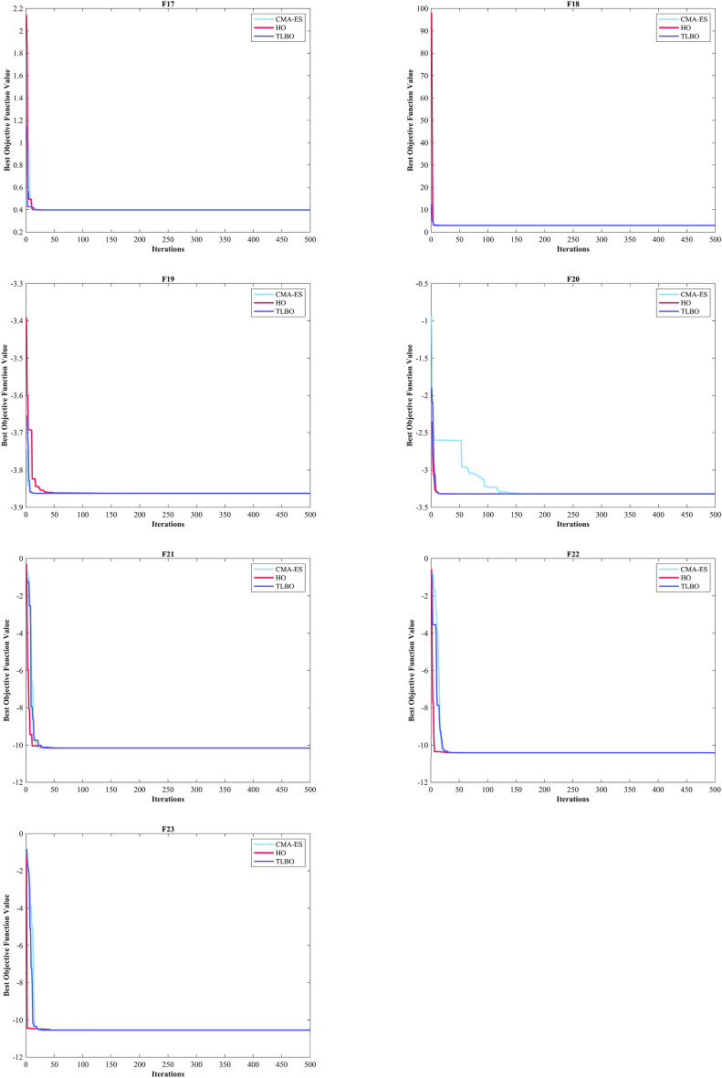
Convergence curves of the top three algorithms in each benchmark functions (F1- F23).
Evaluation benchmark function high-dimensional multimodal
The outcomes of F8-F13 which were HM function using algorithms are presented in Table 3. The objective behind choosing these functions was to assess algorithm’s global search capabilities. The HO outperformed all other algorithms in F8 by a significant margin. In F9, it achieved global optimum along with the WOA, which indicates outstanding performance compared to other algorithms. For F10, it outperformed all other algorithms. F11 converged to global optimum alongside the TLBO, demonstrating superior performance compared to other algorithms. In F12, GOA outperformed HO and TLBO and ranked first. In F13, HO obtained the first rank. For F8, the HO's Std. is notably lower than the investigated algorithms. The F13 Std. is 0.012164, the lowest after the CMA-ES algorithm. This suggests that the HO demonstrates resilience in effectively addressing these functions (Fig. 6).
Table 3.
Evaluation outcomes for the objectives specified in the F8-F13.
| F | M | Optimization algorithms | ||||||||||||
|---|---|---|---|---|---|---|---|---|---|---|---|---|---|---|
| HO | WOA | GWO | SSA | PSO | SCA | FA | GOA | TLBO | CMA-ES | MFO | AOA | IWO | ||
| F8 | Mean | − 12,567 | − 10,876 | − 5568 | − 7033.5 | − 6590.1 | − 3734.5 | − 7463.7 | − 9483.9 | − 7906.9 | − 4363.9 | − 8496.8 | − 5340.9 | -6695.5 |
| Best | − 12,569 | − 12,569 | − 6952.5 | − 8479.5 | − 8325.1 | − 4553.8 | − 8678.6 | − 10,608 | − 9427.3 | − 5177.9 | − 9778.5 | − 6242.2 | -8233.1 | |
| Worst | − 12,530 | − 8345.5 | − 3461 | − 6099.1 | − 4337.3 | − 3362.8 | − 6488.8 | − 8278.2 | − 5915.7 | − 3860.7 | − 6725.5 | − 4587.8 | -4759.4 | |
| Std | 7.3469 | 1729.4 | 941.59 | 640.28 | 903.25 | 281.89 | 615.82 | 556.59 | 781.93 | 320.79 | 863.55 | 471.37 | 677.46 | |
| Median | − 12,569 | − 11,715 | − 5432.2 | − 6845.4 | − 6489.3 | − 3679.7 | − 7454.6 | − 9477.9 | − 8002.1 | − 4301.5 | − 8559.5 | − 5316.7 | -6646.7 | |
| Rank | 1 | 2 | 10 | 7 | 9 | 13 | 6 | 3 | 5 | 12 | 4 | 11 | 8 | |
| F9 | Mean | 0 | 0 | 4.9095 | 52.899 | 45.735 | 50.849 | 186.92 | 202.22 | 12.924 | 126.97 | 155.49 | 0 | 65.852 |
| Best | 0 | 0 | 0 | 23.879 | 22.884 | 0.03564 | 117.41 | 113.44 | 0 | 6.9667 | 84.588 | 0 | 43.819 | |
| Worst | 0 | 0 | 27.59 | 80.591 | 78.602 | 202.58 | 258.69 | 280.58 | 23.007 | 187.18 | 228.14 | 0 | 95.563 | |
| Std | 0 | 0 | 8.2235 | 17.219 | 14.675 | 48.636 | 33.884 | 37.356 | 6.0126 | 71.067 | 40.991 | 0 | 12.894 | |
| Median | 0 | 0 | 5.68-14 | 56.713 | 45.271 | 38.413 | 187.05 | 204.35 | 13.042 | 162.64 | 152.47 | 0 | 64.752 | |
| Rank | 1 | 1 | 2 | 6 | 4 | 5 | 10 | 11 | 3 | 8 | 9 | 1 | 7 | |
| F10 | Mean | 4.44-16 | 4.00-15 | 1.51-14 | 2.7311 | 1.1408 | 14.229 | 18.997 | 19.035 | 9.21-15 | 5.6832-05 | 13.321 | 4.44-16 | 10.679 |
| Best | 4.44-16 | 4.44-16 | 7.55-15 | 1.6462 | 6.26-05 | 0.050121 | 18.271 | 18.094 | 4.00-15 | 3.4412-05 | 0.68917 | 4.44-16 | 0.0087287 | |
| Worst | 4.44-16 | 7.55-15 | 2.18-14 | 5.6781 | 2.4083 | 20.402 | 19.296 | 19.438 | 1.03-13 | 9.5468-05 | 19.962 | 4.44-16 | 19.288 | |
| Std | 0 | 2.47-15 | 3.20-15 | 0.81204 | 0.82655 | 8.6665 | 0.21681 | 0.26647 | 1.79-14 | 1.5424-05 | 7.836 | 0 | 9.4921 | |
| Median | 4.44-16 | 4.00-15 | 1.47-14 | 2.4519 | 1.3404 | 20.204 | 19.028 | 19.088 | 7.55-15 | 5.4007-05 | 17.837 | 4.44-16 | 18.181 | |
| Rank | 1 | 3 | 5 | 8 | 7 | 11 | 12 | 13 | 4 | 6 | 10 | 2 | 9 | |
| F11 | Mean | 0 | 0.012321 | 0.014884 | 0.018205 | 0.021824 | 0.91439 | 163.94 | 0.027115 | 0 | 2.9979-07 | 6.9724 | 0.1554 | 480.41 |
| Best | 0 | 0 | 0 | 0.00077716 | 4.46-07 | 0.025341 | 71.221 | 7.06-05 | 0 | 8.804-08 | 0.43489 | 0.00044758 | 333.51 | |
| Worst | 0 | 0.23384 | 0.15444 | 0.0526 | 0.087692 | 1.6975 | 237.77 | 0.11136 | 0 | 7.7197-07 | 91.085 | 0.43829 | 640.31 | |
| Std | 0 | 0.048624 | 0.033114 | 0.011469 | 0.026358 | 0.42847 | 36.504 | 0.028254 | 0 | 1.7512-07 | 22.846 | 0.11095 | 71.029 | |
| Median | 0 | 0 | 0 | 0.016869 | 0.0098613 | 0.99061 | 163.4 | 0.01876 | 0 | 2.6344-07 | 1.0093 | 0.13784 | 477.65 | |
| Rank | 1 | 3 | 4 | 5 | 6 | 9 | 11 | 7 | 1 | 2 | 10 | 8 | 12 | |
| F12 | Mean | 9.30-09 | 0.020187 | 0.1456 | 7.0883 | 0.11094 | 40,328 | 42.51 | 4.4816 | 0.0034654 | 1.9945-09 | 17.719 | 0.51896 | 8.8769 |
| Best | 1.49-09 | 0.0024683 | 0.034516 | 1.4549 | 6.84-09 | 0.79446 | 13.932 | 1.37-10 | 6.74-09 | 7.8685-10 | 0.70708 | 0.41734 | 3.4841 | |
| Worst | 7.32-08 | 0.14187 | 0.31253 | 16.042 | 1.0405 | 7.11E + 05 | 76.246 | 14.181 | 0.10367 | 7.2421-09 | 285.16 | 0.61102 | 12.625 | |
| Std | 1.62-08 | 0.025008 | 0.067403 | 3.1194 | 0.23009 | 1.47E + 05 | 15.85 | 3.6815 | 0.018926 | 1.3528-09 | 50.987 | 0.050388 | 1.8974 | |
| Median | 5.33-09 | 0.013983 | 0.14025 | 6.8009 | 2.09-05 | 17.858 | 44.103 | 3.5971 | 1.14-07 | 1.6197-09 | 6.8694 | 0.527 | 8.9038 | |
| Rank | 2 | 4 | 6 | 9 | 5 | 13 | 12 | 8 | 3 | 1 | 11 | 7 | 10 | |
| F13 | Mean | 0.0050467 | 0.44897 | 1.4596 | 18.841 | 0.021928 | 6.69E + 05 | 44,205 | 0.49606 | 0.072491 | 2.128-08 | 2.73E + 07 | 2.81 | 0.0027154 |
| Best | 1.35-32 | 0.14522 | 0.80982 | 0.033744 | 1.03-08 | 2.7393 | 50.302 | 1.80-10 | 2.23-06 | 7.311-09 | 2.1321 | 2.6101 | 5.00E-05 | |
| Worst | 0.063492 | 1.3863 | 1.8467 | 62.222 | 0.28572 | 1.31E + 07 | 3.97E + 05 | 4.9234 | 0.20724 | 4.3763-08 | 4.10E + 08 | 2.9954 | 0.011275 | |
| Std | 0.012164 | 0.27245 | 0.21244 | 15.746 | 0.05445 | 2.56E + 06 | 86,550 | 1.2302 | 0.069667 | 9.3747-09 | 1.04E + 08 | 0.092163 | 0.0047482 | |
| Median | 0.0014522 | 0.35799 | 1.4967 | 18.36 | 0.010988 | 1130.3 | 2772.3 | 0.010987 | 0.047853 | 1.9344-08 | 29.131 | 2.7955 | 0.00014517 | |
| Rank | 3 | 6 | 8 | 10 | 4 | 12 | 11 | 7 | 5 | 1 | 13 | 9 | 2 | |
| Sum rank | 9 | 19 | 35 | 45 | 35 | 63 | 62 | 49 | 21 | 30 | 57 | 38 | 48 | |
| Mean rank | 1.5 | 3.1667 | 5.8333 | 7.5000 | 5.8333 | 10.5 | 10.3333 | 8.1667 | 3.5 | 5 | 9.5 | 6.3333 | 8 | |
| Total rank | 1 | 2 | 5 | 8 | 6 | 13 | 12 | 10 | 3 | 4 | 11 | 7 | 9 | |
Evaluation fixed-dimension multimodal benchmark function
The objective was to examine the algorithm’s capacity to achieve a harmonious equilibrium between exploration and exploitation while conducting the search procedure on F14-F23. Results are reported in Table 4. HO performed best for F14-F23. The HO achieves a significantly lower Std. especially for F20-F22. The findings suggest that HO, characterized by its strong capability to balance exploration and exploitation, demonstrates superior performance when addressing FM and MM functions.
Table 4.
Evaluation outcomes for the objectives specified in the F14-F23.
| F | M | Optimization algorithms | ||||||||||||
|---|---|---|---|---|---|---|---|---|---|---|---|---|---|---|
| HO | WOA | GWO | SSA | PSO | SCA | FA | GOA | TLBO | CMA-ES | MFO | AOA | IWO | ||
| F14 | Mean | 0.998 | 3.0928 | 6.9207 | 1.1305 | 5.5195 | 2.2512 | 9.502 | 12.782 | 0.998 | 4.7816 | 2.51 | 8.0876 | 11.358 |
| Best | 0.998 | 0.998 | 0.998 | 0.998 | 0.998 | 0.998 | 0.998 | 0.998 | 0.998 | 1.992 | 0.998 | 0.998 | 0.998 | |
| Worst | 0.998 | 10.763 | 12.671 | 1.992 | 12.671 | 10.763 | 21.988 | 23.809 | 0.998 | 11.721 | 10.763 | 12.671 | 23.809 | |
| Std | 0 | 3.2723 | 4.9187 | 0.34368 | 3.0682 | 1.8878 | 6.2553 | 6.298 | 3.86-16 | 2.4391 | 2.3156 | 4.7721 | 7.3331 | |
| Median | 0.998 | 1.495 | 7.3657 | 0.998 | 5.9288 | 2.0092 | 8.3574 | 12.671 | 0.998 | 3.9742 | 0.998 | 10.763 | 10.763 | |
| Rank | 1 | 6 | 9 | 3 | 8 | 4 | 11 | 13 | 2 | 7 | 5 | 10 | 12 | |
| F15 | Mean | 0.00030836 | 0.00088694 | 0.0083127 | 0.0027545 | 0.0024923 | 0.0010454 | 0.0058617 | 0.010286 | 0.00036839 | 0.0019 | 0.0013293 | 0.0071685 | 0.0027859 |
| Best | 0.00030749 | 0.00030755 | 0.00030749 | 0.00033385 | 0.00030749 | 0.00057375 | 0.00030749 | 0.00030749 | 0.00030749 | 0.0011 | 0.00074582 | 0.00034241 | 0.00058505 | |
| Worst | 0.00031288 | 0.0035616 | 0.056621 | 0.02043 | 0.020363 | 0.0016389 | 0.020363 | 0.056543 | 0.0012232 | 0.0035 | 0.0083337 | 0.069975 | 0.020363 | |
| Std | 1.31-06 | 0.00071966 | 0.012961 | 0.0059824 | 0.0060732 | 0.00035949 | 0.0089054 | 0.012603 | 0.00018223 | 7.25-06 | 0.0013978 | 0.014639 | 0.0059637 | |
| Median | 0.00030779 | 0.0005872 | 0.00045554 | 0.00077266 | 0.00030782 | 0.00087851 | 0.00030749 | 0.0029582 | 0.00030749 | 0.0016 | 0.00080207 | 0.00047392 | 0.00074539 | |
| Rank | 1 | 3 | 12 | 8 | 7 | 4 | 10 | 13 | 2 | 6 | 5 | 11 | 9 | |
| F16 | Mean | − 1.0316 | − 1.0316 | − 1.0316 | − 1.0316 | − 1.0316 | − 1.0316 | − 0.8956 | − 0.79107 | − 1.0316 | − 1.0316 | − 1.0316 | − 1.0316 | − 1.0316 |
| Best | − 1.0316 | − 1.0316 | − 1.0316 | − 1.0316 | − 1.0316 | − 1.0316 | − 1.0316 | − 1.0316 | − 1.0316 | − 1.0316 | − 1.0316 | − 1.0316 | − 1.0316 | |
| Worst | − 1.0316 | − 1.0316 | − 1.0316 | − 1.0316 | − 1.0316 | − 1.0314 | − 0.21546 | 2.1043 | − 1.0316 | − 1.0316 | − 1.0316 | − 1.0316 | − 1.0316 | |
| Std | 5.96-16 | 3.09-09 | 9.67-09 | 2.66-14 | 6.71-16 | 5.70-05 | 0.30937 | 0.62776 | 6.65-16 | 6.78-16 | 6.78-16 | 1.22-07 | 1.44-08 | |
| Median | − 1.0316 | − 1.0316 | − 1.0316 | − 1.0316 | − 1.0316 | − 1.0316 | − 1.0316 | − 1.0316 | − 1.0316 | − 1.0316 | − 1.0316 | − 1.0316 | − 1.0316 | |
| Rank | 1 | 1 | 1 | 1 | 1 | 1 | 2 | 3 | 1 | 1 | 1 | 1 | 1 | |
| F17 | Mean | 0.39789 | 0.3979 | 0.39789 | 0.39789 | 0.39789 | 0.40008 | 0.39789 | 0.39789 | 0.39789 | 0.39789 | 0.39789 | 0.41197 | 0.39789 |
| Best | 0.39789 | 0.39789 | 0.39789 | 0.39789 | 0.39789 | 0.3979 | 0.39789 | 0.39789 | 0.39789 | 0.39789 | 0.39789 | 0.39813 | 0.39789 | |
| Worst | 0.39789 | 0.39794 | 0.39789 | 0.39789 | 0.39789 | 0.40747 | 0.39789 | 0.39789 | 0.39789 | 0.39789 | 0.39789 | 0.4415 | 0.39789 | |
| Std | 0 | 1.42-05 | 1.41-06 | 4.70-14 | 7.23-16 | 0.0023394 | 3.86-11 | 0 | 0 | 0 | 0 | 0.01286 | 5.57-09 | |
| Median | 0.39789 | 0.39789 | 0.39789 | 0.39789 | 0.39789 | 0.39939 | 0.39789 | 0.39789 | 0.39789 | 0.39789 | 0.39789 | 0.40712 | 0.39789 | |
| Rank | 1 | 2 | 1 | 1 | 1 | 3 | 1 | 1 | 1 | 1 | 1 | 4 | 1 | |
| F18 | Mean | 3 | 3.0001 | 3 | 3 | 3.9 | 3.0001 | 3.9 | 9.3 | 3 | 3 | 3 | 7.7674 | 3 |
| Best | 3 | 3 | 3 | 3 | 3 | 3 | 3 | 3 | 3 | 3 | 3 | 3 | 3 | |
| Worst | 3 | 3.0006 | 3.0001 | 3 | 30 | 3.0004 | 30 | 84 | 3 | 3 | 3 | 37.986 | 3 | |
| Std | 1.27-15 | 0.00013473 | 1.79-05 | 2.77-13 | 4.9295 | 0.00010081 | 4.9295 | 16.904 | 5.53-16 | 1.35-15 | 1.62-15 | 10.92 | 8.47-07 | |
| Median | 3 | 3 | 3 | 3 | 3 | 3 | 3 | 3 | 3 | 3 | 3 | 3 | 3 | |
| Rank | 1 | 2 | 1 | 1 | 3 | 2 | 3 | 5 | 1 | 1 | 1 | 4 | 1 | |
| F | M | Optimization algorithms | ||||||||||||
|---|---|---|---|---|---|---|---|---|---|---|---|---|---|---|
| HO | WOA | GWO | SSA | PSO | SCA | FA | GOA | TLBO | CMA-ES | MFO | AOA | IWO | ||
| F19 | Mean | − 3.8628 | − 3.8335 | − 3.8595 | − 3.8628 | − 3.8628 | − 3.8542 | − 3.8628 | − 3.8212 | − 3.8628 | − 3.8628 | − 3.8628 | − 3.8512 | -3.8628 |
| Best | − 3.8628 | − 3.8628 | − 3.8628 | − 3.8628 | − 3.8628 | − 3.8621 | − 3.8628 | − 3.8628 | − 3.8628 | − 3.8628 | − 3.8628 | − 3.8605 | -3.8628 | |
| Worst | − 3.8628 | − 3.0885 | − 3.8549 | − 3.8628 | − 3.8628 | − 3.8443 | − 3.8628 | − 3.0898 | − 3.8628 | − 3.8628 | − 3.8628 | − 3.8408 | -3.8628 | |
| Std | 2.70-15 | 0.14079 | 0.0036479 | 1.51-11 | 6.42-07 | 0.0032649 | 5.72-11 | 0.14271 | 2.71-15 | 2.71-15 | 2.71-15 | 0.0038724 | 6.32-07 | |
| Median | − 3.8628 | − 3.8611 | − 3.8624 | − 3.8628 | − 3.8628 | − 3.8542 | − 3.8628 | − 3.8627 | − 3.8628 | − 3.8628 | − 3.8628 | − 3.8516 | − 3.8628 | |
| Rank | 1 | 5 | 2 | 1 | 1 | 3 | 1 | 6 | 1 | 1 | 1 | 4 | 1 | |
| F20 | Mean | − 3.322 | − 3.2406 | − 3.1218 | − 3.2275 | − 3.2784 | − 2.8823 | − 3.2586 | − 2.7966 | − 3.2811 | − 3.2919 | − 3.2422 | − 3.0755 | − 3.203 |
| Best | − 3.322 | − 3.3219 | − 3.322 | − 3.322 | − 3.322 | − 3.1473 | − 3.322 | − 3.3138 | − 3.3206 | − 3.322 | − 3.322 | − 3.1844 | − 3.2031 | |
| Worst | − 3.322 | − 2.4308 | − 2.2671 | − 3.1469 | − 3.2031 | − 1.9133 | − 3.2031 | − 1.9056 | − 3.1059 | − 3.2031 | − 3.1376 | − 2.9507 | − 3.2026 | |
| Std | 9.78-12 | 0.17522 | 0.26562 | 0.058906 | 0.058273 | 0.32598 | 0.060328 | 0.36014 | 0.066162 | 0.051459 | 0.063837 | 0.063759 | 0.00012908 | |
| Median | − 3.322 | − 3.3191 | − 3.1676 | − 3.1988 | − 3.322 | − 2.9914 | − 3.2031 | − 2.9387 | − 3.3109 | − 3.322 | − 3.2031 | − 3.0905 | − 3.2031 | |
| Rank | 1 | 7 | 10 | 8 | 4 | 12 | 5 | 13 | 3 | 2 | 6 | 11 | 9 | |
| F21 | Mean | − 10.153 | − 7.9465 | − 8.6325 | − 7.5665 | − 6.3165 | − 2.1516 | − 5.6345 | − 5.2171 | − 9.778 | − 7.9121 | − 6.3132 | − 3.4351 | − 6.6391 |
| Best | − 10.153 | − 10.153 | − 10.153 | − 10.153 | − 10.153 | − 6.0051 | − 10.153 | − 10.153 | − 10.153 | − 10.153 | − 10.153 | − 5.5613 | − 10.153 | |
| Worst | − 10.153 | − 2.6294 | − 5.0552 | − 2.6305 | − 2.6305 | − 0.35136 | − 2.6305 | − 2.6305 | − 3.9961 | − 2.6829 | − 2.6305 | − 1.9507 | − 2.6305 | |
| Std | 4.74-06 | 2.7979 | 2.3619 | 3.5062 | 3.6985 | 1.872 | 3.1766 | 2.9687 | 1.4345 | 3.4819 | 3.5169 | 0.97125 | 3.4561 | |
| Median | − 10.153 | − 10.137 | − 10.152 | − 10.153 | − 5.078 | − 0.88031 | − 5.0552 | − 5.0552 | − 10.153 | − 10.153 | − 5.078 | − 3.2531 | − 5.1008 | |
| Rank | 1 | 4 | 3 | 6 | 8 | 13 | 10 | 11 | 2 | 5 | 9 | 12 | 6 | |
| F22 | Mean | − 10.403 | − 6.573 | − 9.5722 | − 8.8874 | − 6.7572 | − 2.7098 | − 5.3848 | − 5.5286 | − 9.7141 | − 10.403 | − 8.2382 | − 3.7002 | − 7.4415 |
| Best | − 10.403 | − 10.401 | − 10.403 | − 10.403 | − 10.403 | − 6.3217 | − 10.403 | − 10.403 | − 10.403 | − 10.403 | − 10.403 | − 6.8593 | − 10.403 | |
| Worst | − 10.403 | − 1.8372 | − 2.7659 | − 2.7519 | − 1.8376 | − 0.52104 | − 1.8376 | − 1.8376 | − 5.0265 | − 10.403 | − 2.7519 | − 1.2708 | − 1.8376 | |
| Std | 6.16-05 | 3.2924 | 2.1838 | 2.8452 | 3.7466 | 1.9244 | 3.194 | 3.3448 | 1.7896 | 1.65-15 | 3.3738 | 1.2624 | 3.7449 | |
| Median | − 10.403 | − 5.0875 | − 10.402 | − 10.403 | − 7.7659 | − 2.6079 | − 3.7243 | − 3.7243 | − 10.403 | − 10.403 | − 10.403 | − 3.6181 | − 10.403 | |
| Rank | 1 | 9 | 3 | 5 | 8 | 13 | 11 | 10 | 2 | 1 | 6 | 12 | 7 | |
| F23 | Mean | − 10.536 | − 6.8188 | − 9.2737 | − 8.2567 | − 6.0645 | − 4.1564 | − 4.7569 | − 5.3577 | − 10.123 | − 10.536 | − 7.9819 | − 4.6738 | − 8.3548 |
| Best | − 10.536 | − 10.534 | − 10.536 | − 10.536 | − 10.536 | − 8.3393 | − 10.536 | − 10.536 | − 10.536 | − 10.536 | − 10.536 | − 8.6767 | − 10.536 | |
| Worst | − 10.536 | − 1.8588 | − 2.4217 | − 2.4217 | − 1.8595 | − 0.94428 | − 1.6766 | − 1.8595 | − 3.8354 | − 10.536 | − 2.4217 | − 1.8573 | − 2.4217 | |
| Std | 2.99-05 | 3.4247 | 2.9055 | 3.3562 | 3.7424 | 1.5765 | 3.0762 | 3.5273 | 1.5801 | 1.78-15 | 3.6868 | 1.5405 | 3.437 | |
| Median | − 10.536 | − 5.1284 | − 10.536 | − 10.536 | − 3.8354 | − 4.6344 | − 3.8354 | − 3.8354 | − 10.536 | − 10.536 | − 10.536 | − 4.8892 | − 10.536 | |
| Rank | 1 | 8 | 4 | 6 | 9 | 13 | 11 | 10 | 2 | 1 | 7 | 12 | 5 | |
| Sum rank | 10 | 47 | 46 | 40 | 50 | 68 | 65 | 85 | 17 | 26 | 42 | 81 | 52 | |
| Mean rank | 1 | 4.7000 | 4.6000 | 4 | 5 | 6.8000 | 6.5000 | 8.5000 | 1.7000 | 2.6000 | 4.2000 | 8.1000 | 5.2000 | |
| Total rank | 1 | 7 | 6 | 4 | 8 | 11 | 10 | 13 | 2 | 3 | 5 | 12 | 9 | |
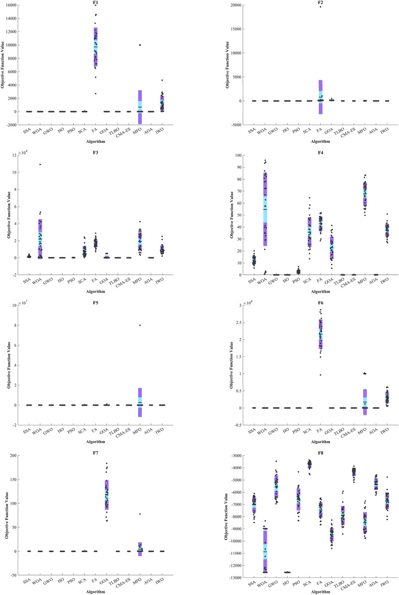
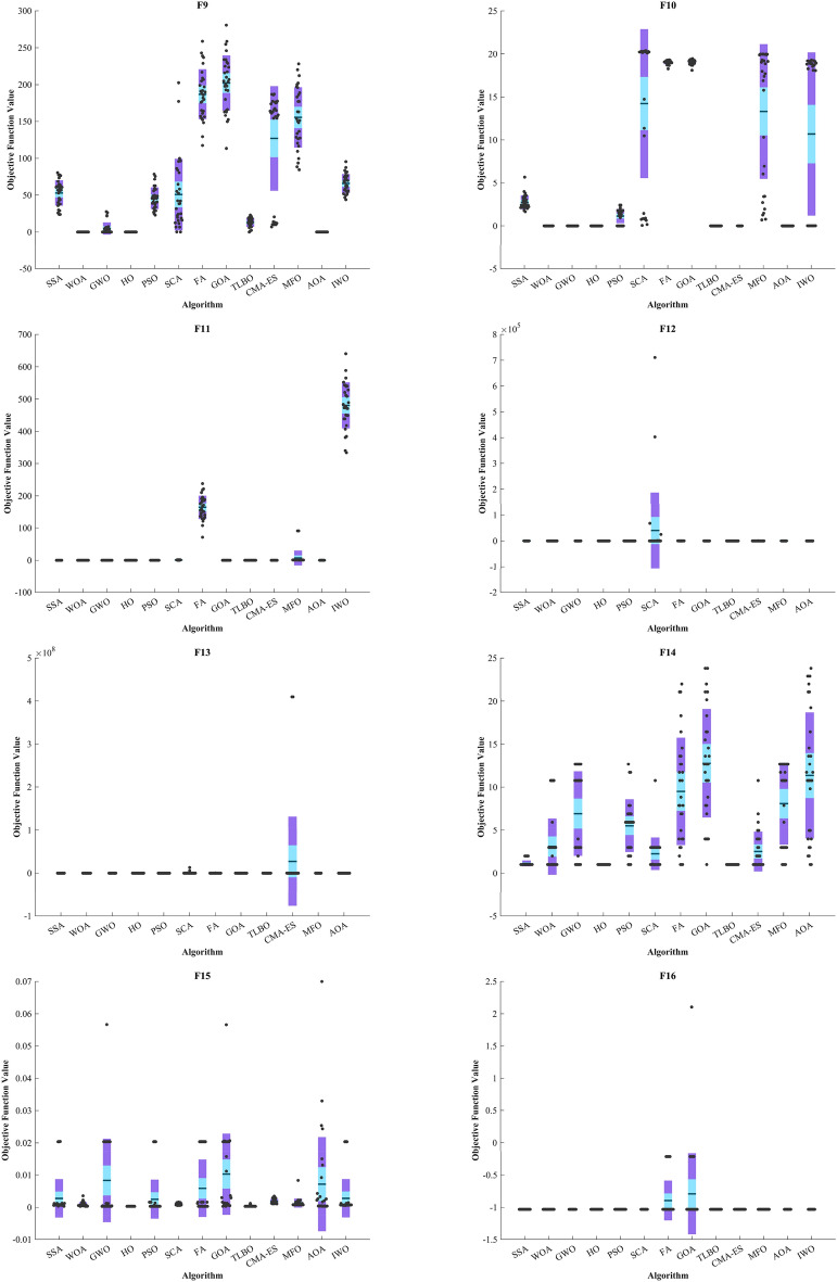
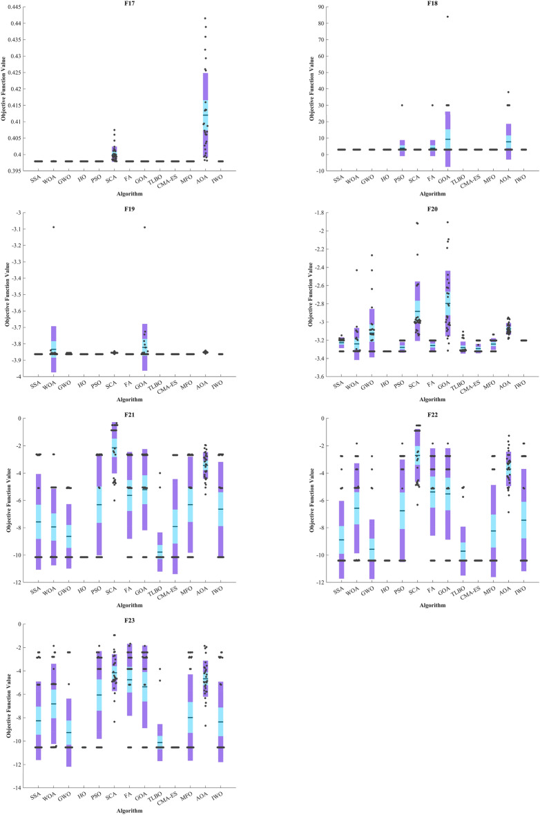
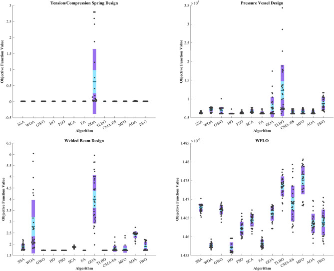
Figure 5 displays box plot diagrams depicting the optimal values of the objective function obtained from 30 separate runs for F1-F23, utilizing a set of HO and 12 algorithms.
Figure 5.
Boxplot illustrating the performance of the HO in comparison to competing algorithms for optimizing BFs (F1-F23).
Evaluation of the ZP
Kudela and Matousek introduced eight novel challenging benchmark functions, presenting a formidable challenge for bound-constrained single-objective optimization. These functions are crafted on the foundation of a ZP characterized by their non-differentiable nature and remarkable multimodality, and introduced functions incorporate three adjustable parameters, allowing for alterations in their behavior and level of difficulty137. Table 5 presents the results for eight ZP (ZP-F1 to ZP-F8). In ZP-F1 and ZP-F2, WOA outperformed HO and TLBO and ranked first. The HO exhibited superior performance across ZP-F3 to ZP-F8, achieving global optimum for the objective function in ZP-F3 and ZP-F8. HO outperformed all investigated algorithms for ZP-F3 and ZP-F4. Furthermore, the HO achieved a remarkable result by achieving global optimum for ZP-F5 and ZP-F6 across all criteria. In the case of ZP-F7, HO was in close competition with the GWO algorithm and secured the first rank by achieving global optimum. A similar success was observed for the ZP-F8 function, where HO competed with the AOA algorithm and achieved global optimum (Fig. 6).
Table 5.
Evaluation outcomes for the objectives specified in the ZP.
| F | M | Optimization Algorithms | ||||||||||||
|---|---|---|---|---|---|---|---|---|---|---|---|---|---|---|
| HO | WOA | GWO | SSA | PSO | SCA | FA | GOA | TLBO | CMA-ES | MFO | AOA | IWO | ||
| ZP-F1 | Mean | 5.81E-66 | 3.70E-63 | 126.21 | 401.46 | 103.82 | 599.72 | 499.05 | 295.46 | 7.60E-39 | 570.29 | 394.48 | 0.20819 | 483.88 |
| Best | 5.47E-72 | 0 | 8.54E-27 | 302.31 | 72.97 | 390.51 | 383.14 | 227.12 | 5.90E-40 | 488.94 | 326.44 | 5.30E-05 | 428.22 | |
| Worst | 6.08E-65 | 9.86E-62 | 686.76 | 528.15 | 132.22 | 821.23 | 576.72 | 414.65 | 7.28E-38 | 630.04 | 529.95 | 0.59081 | 574.49 | |
| Std | 1.51E-65 | 1.80E-62 | 194.58 | 53.315 | 16.449 | 111.11 | 44.155 | 46.643 | 1.55E-38 | 34.272 | 45.389 | 0.16611 | 39.582 | |
| Median | 1.17E-67 | 3.29E-65 | 20.172 | 390.45 | 100.2 | 613.96 | 501.48 | 290.25 | 3.14E-39 | 570.84 | 388.78 | 0.1819 | 478.19 | |
| Rank | 1 | 2 | 6 | 9 | 5 | 13 | 11 | 7 | 3 | 12 | 8 | 4 | 10 | |
| ZP-F2 | Mean | 2.86E-65 | 9.29E-64 | 0.057452 | 411.24 | 167.96 | 464.66 | 1.36E-39 | 946.55 | 694.82 | 524.24 | 673.65 | 0.24434 | 919.95 |
| Best | 2.50E-71 | 0 | 6.23E-27 | 326.33 | 118.88 | 181.41 | 3.70E-40 | 843.24 | 579.84 | 328.51 | 518.82 | 0.00025022 | 680.28 | |
| Worst | 4.92E-64 | 1.78E-62 | 1.7235 | 500.21 | 244.4 | 707.21 | 5.42E-39 | 1065.3 | 808.5 | 640.74 | 861.43 | 0.62708 | 1094.2 | |
| Std | 9.69E-65 | 3.28E-63 | 0.31468 | 40.297 | 27.671 | 140.48 | 1.12E-39 | 58.929 | 66.872 | 63.56 | 70.097 | 0.17334 | 82.853 | |
| Median | 3.14E-67 | 3.24E-65 | 4.47E-26 | 407.95 | 164.04 | 470.97 | 9.71E-40 | 943.5 | 681.74 | 543.1 | 672.55 | 0.23486 | 914.94 | |
| Rank | 1 | 2 | 4 | 7 | 6 | 8 | 3 | 13 | 11 | 9 | 10 | 5 | 12 | |
| ZP-F3 | Mean | 1.66E-60 | 1.57E-54 | 55.432 | 549.6 | 305.04 | 548.83 | 491.76 | 543.73 | 493.46 | 702.89 | 387.35 | 536.12 | 0.17836 |
| Best | 0 | 2.26E-70 | 5.29E-27 | 520.92 | 223.48 | 125.47 | 474.81 | 461.05 | 389.78 | 674.68 | 356.77 | 478.31 | 6.41E-05 | |
| Worst | 1.97E-59 | 4.25E-53 | 622.76 | 572.28 | 405.51 | 601.45 | 502.87 | 609.37 | 576.5 | 640.74 | 444.61 | 586.16 | 0.49694 | |
| Std | 4.60E-60 | 7.77E-54 | 134.96 | 13.521 | 46.236 | 105 | 7.7342 | 33.124 | 43.534 | 12.79 | 18.204 | 22.927 | 0.13407 | |
| Median | 3.78E-64 | 3.18E-66 | 14.392 | 548.5 | 306.76 | 577.19 | 491.54 | 548.19 | 491.79 | 703.89 | 386.52 | 535.44 | 0.18738 | |
| Rank | 1 | 2 | 4 | 12 | 5 | 11 | 7 | 10 | 8 | 13 | 6 | 9 | 3 | |
| ZP-F4 | Mean | 8.84E-52 | 15.063 | 13.2 | 580.13 | 240.08 | 281.78 | 565.75 | 486.58 | 485.52 | 659.77 | 399.81 | 0.31674 | 460.65 |
| Best | 0 | 3.83E-69 | 9.80E-27 | 407.46 | 168.95 | 20.976 | 555.51 | 422.48 | 404 | 633.74 | 351.62 | 0.0081653 | 417.49 | |
| Worst | 2.65E-50 | 220.31 | 47.416 | 606.17 | 308.15 | 596.39 | 569.78 | 564.8 | 543.55 | 678.56 | 467.78 | 0.63772 | 526.23 | |
| Std | 4.84E-51 | 46.111 | 11.422 | 36.235 | 34.131 | 220.52 | 2.9162 | 30.404 | 33.984 | 10.471 | 28.016 | 0.17113 | 26.368 | |
| Median | 1.09E-63 | 5.73E-66 | 14.42 | 588.77 | 235.18 | 189.01 | 566.01 | 483.73 | 485.59 | 661.44 | 396.32 | 0.35609 | 458.52 | |
| Rank | 1 | 4 | 3 | 12 | 5 | 6 | 11 | 10 | 9 | 13 | 7 | 2 | 8 | |
| F | M | Optimization Algorithms | ||||||||||||
|---|---|---|---|---|---|---|---|---|---|---|---|---|---|---|
| HO | WOA | GWO | SSA | PSO | SCA | FA | GOA | TLBO | CMA-ES | MFO | AOA | IWO | ||
| ZP-F5 | Mean | 0 | 273.38 | 464.21 | 1718.6 | 1297 | 1467.7 | 1766.1 | 1047.9 | 1496.1 | 2480.4 | 1573.9 | 11.263 | 1724.3 |
| Best | 0 | 0 | 47.775 | 1583.7 | 1148.2 | 607.85 | 1527 | 867.71 | 1298.4 | 2380.2 | 1231.4 | 3.30E-06 | 1606.1 | |
| Worst | 0 | 1366.9 | 1747.3 | 1955.4 | 1545 | 1970.3 | 1939.1 | 1465.7 | 1664.3 | 2531.1 | 1793.3 | 41.375 | 1856 | |
| Std | 0 | 463.47 | 531.54 | 94.576 | 93.791 | 358.18 | 99.787 | 144.98 | 80.878 | 35.674 | 119.7 | 10.591 | 73.998 | |
| Median | 0 | 3.55E-15 | 195.54 | 1703.1 | 1276.3 | 1599.3 | 1750.6 | 1009.5 | 1480.4 | 2478 | 1596.1 | 8.8444 | 1720.1 | |
| Rank | 1 | 3 | 4 | 10 | 6 | 7 | 12 | 5 | 8 | 13 | 9 | 2 | 11 | |
| ZP-F6 | Mean | 0 | 2.37E-16 | 28.129 | 1301.6 | 962.94 | 683.03 | 1413.4 | 1364.8 | 1497.9 | 2480.4 | 1384.8 | 0.0099571 | 1522.5 |
| Best | 0 | 0 | 2.84E-14 | 1118.9 | 771.93 | 171.18 | 1213.9 | 1229.3 | 1117.4 | 2303.3 | 1250.7 | 1.44E-11 | 1353.3 | |
| Worst | 0 | 3.55E-15 | 141.92 | 1530.8 | 1323.8 | 1889.9 | 1559.3 | 1577.3 | 1952.8 | 2500 | 1499.8 | 0.13786 | 1672.1 | |
| Std | 0 | 9.01E-16 | 44.749 | 101.86 | 120.91 | 404.33 | 74.498 | 95.834 | 191.33 | 47.699 | 72.837 | 0.02644 | 76.638 | |
| Median | 0 | 0 | 7.99E-14 | 1289.6 | 943.67 | 619.83 | 1414.6 | 1353.6 | 1482 | 2445.1 | 1376.6 | 0.00019612 | 1530.1 | |
| Rank | 1 | 2 | 4 | 7 | 6 | 5 | 10 | 8 | 11 | 13 | 9 | 3 | 12 | |
| ZP-F7 | Mean | 1.28E-12 | 66.15 | 2.30E-10 | 4009.7 | 3401.1 | 204.52 | 4485.6 | 4362.2 | 3278.3 | 4756.4 | 3913.5 | 0.047242 | 4391.5 |
| Best | 0 | 0 | 7.67E-11 | 3885.1 | 3250.3 | 0.38829 | 4382.1 | 4273.7 | 0 | 4464.1 | 3831.7 | 0 | 4293.2 | |
| Worst | 1.92E-11 | 1984.5 | 3.93E-10 | 4148.9 | 3531.1 | 1016.7 | 4604.8 | 4583.2 | 4209.2 | 4864.5 | 4040.4 | 1.0943 | 4556 | |
| Std | 4.16E-12 | 362.32 | 7.44E-11 | 70.365 | 68.54 | 197.33 | 47.575 | 83.923 | 1162.8 | 103.69 | 41.426 | 0.2002 | 57.296 | |
| Median | 0 | 0 | 2.40E-10 | 4012.9 | 3405 | 154.3 | 4482.8 | 4329.8 | 3563.4 | 4798.3 | 3916 | 8.64E-05 | 4388.1 | |
| Rank | 1 | 4 | 2 | 9 | 7 | 5 | 12 | 10 | 6 | 13 | 8 | 3 | 11 | |
| ZP-F8 | Mean | 2.2833 | 304.89 | 1805 | 1193 | 1686.4 | 1256.1 | 1780.1 | 1680.8 | 549.37 | 2522.8 | 533.77 | 4.5963 | 1804.4 |
| Best | 0 | 273.11 | 1687.5 | 1102.7 | 1366.5 | 1130.3 | 1578.5 | 1451.6 | 537.65 | 2425.3 | 507.73 | 1.55E-08 | 1643 | |
| Worst | 68.5 | 429.47 | 1961.5 | 1279.8 | 2049.9 | 1369.1 | 2012.8 | 1824.7 | 552.32 | 2574.5 | 702.13 | 31.634 | 2006.8 | |
| Std | 12.506 | 46.077 | 68.209 | 53.834 | 182.4 | 59.606 | 103.17 | 84.747 | 3.1924 | 103.69 | 39.594 | 8.7473 | 79.751 | |
| Median | 0 | 277.4 | 1794.4 | 1198.8 | 1680.1 | 1249 | 1795 | 1661.2 | 549.77 | 2527.3 | 523.8 | 0.0024046 | 1800.5 | |
| Rank | 1 | 3 | 12 | 6 | 9 | 7 | 10 | 8 | 5 | 13 | 4 | 2 | 11 | |
| Sum rank | 8 | 22 | 39 | 72 | 49 | 62 | 76 | 71 | 61 | 99 | 61 | 30 | 78 | |
| Mean rank | 1 | 2.7500 | 4.875 | 9 | 6.1200 | 7.7500 | 9.5000 | 8.8750 | 7.6250 | 12.375 | 7.6250 | 3.7500 | 9.7500 | |
| Total rank | 1 | 2 | 4 | 10 | 5 | 8 | 11 | 9 | 6 | 13 | 7 | 3 | 12 | |
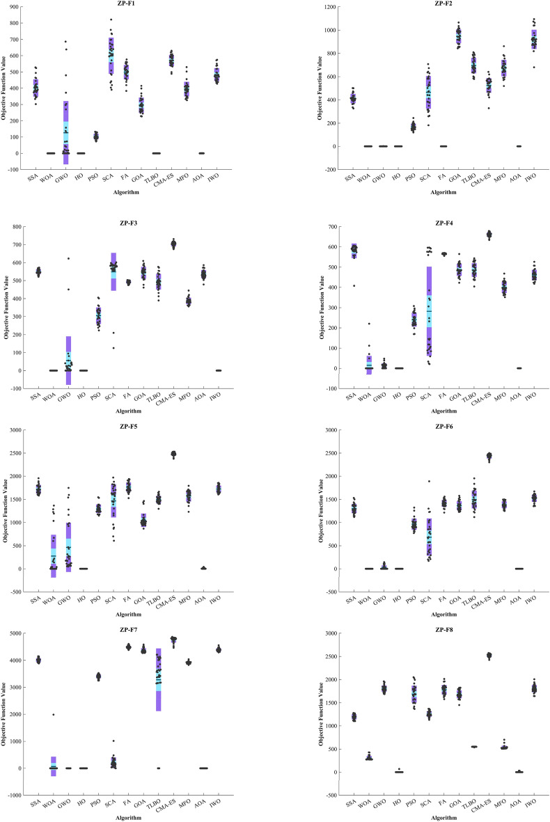
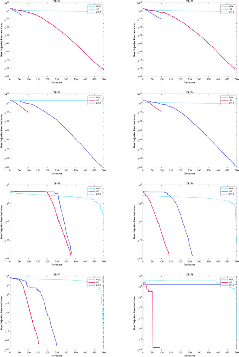
In addition, when examining the boxplot diagrams in Fig. 7, it is evident that the HO consistently demonstrated a lower Std. than other algorithms. Figure 8, covering ZP-F1 to ZP-F8, demonstrates that the HO performs much faster than its competitors and reaches an unattainable optimal solution for other investigated algorithms.
Figure 7.
Boxplot illustrating the performance of the HO in comparison to competing algorithms for ZP.
Figure 8.
Convergence curves of the top three algorithms in each function in ZP.
Evaluation of the CEC 2019 test suite
CEC 2019 test BFs include ten complex functions described in138. The details of optimization are reported in Table 6. C19–F1 and C19–F10 functions from the CEC 2019 test designed for single-objective real parameter optimization. They aim to find the best possible outcome globally. These functions are ideal for assessing how well algorithms can perform in a thorough search for the best solution. The HO achieved the top rank in C19-F2–C19-F4 and C19-F7 functions. In C19-F1, it notably outperformed other algorithms across all criteria except the Best criterion Similar outcomes were observed in C19-F2, which ranked first with 3 top algorithms in converges (HO, PSO and SSA). The GWO achieved the top rank in C19-F1. In the case of C19-F3, HO secured the first position with a Std. better than that of the SSA algorithm. For C19-F4, both the Best and Mean criteria demonstrated significantly superior values compared to other algorithms. In C19-F5 CMA-ES surpassed of all algorithms.
Table 6.
Evaluation outcomes for the objectives specified in the CEC 2019.
| F | M | Optimization Algorithms | ||||||||||||
|---|---|---|---|---|---|---|---|---|---|---|---|---|---|---|
| HO | WOA | GWO | SSA | PSO | SCA | FA | GOA | TLBO | CMA-ES | MFO | AOA | IWO | ||
| C19-F1 | Mean | 47,252 | 1.79E + 10 | 3.52E + 07 | 1.06E + 10 | 5.21E + 08 | 8.36E + 09 | 3.87E + 10 | 3.71E + 10 | 1.19E + 08 | 3.5331e + 09 | 1.75E + 10 | 2.45E + 09 | 9.13E + 12 |
| Best | 39,398 | 8.47E + 05 | 38,806 | 5.95E + 08 | 3.31E + 07 | 3.43E + 08 | 1.38E + 09 | 1.83E + 09 | 8.13E + 06 | 4.5975e + 08 | 6.17E + 08 | 7.78E + 05 | 7.70E + 10 | |
| Worst | 55,445 | 1.81E + 11 | 2.53E + 08 | 3.42E + 10 | 2.15E + 09 | 4.01E + 10 | 2.76E + 11 | 1.05E + 11 | 7.17E + 08 | 1.875e + 10 | 1.11E + 11 | 4.64E + 10 | 5.93E + 13 | |
| Std | 4020 | 3.93E + 10 | 7.03E + 07 | 1.01E + 10 | 4.90E + 08 | 9.63E + 09 | 7.23E + 10 | 3.20E + 10 | 1.40E + 08 | 3.3022e + 09 | 2.50E + 10 | 8.61E + 09 | 1.25E + 13 | |
| Median | 46,563 | 1.79E + 08 | 1.19E + 06 | 7.07E + 09 | 4.16E + 08 | 4.32E + 09 | 1.16E + 10 | 3.22E + 10 | 8.72E + 07 | 2.9352e + 09 | 8.52E + 09 | 3.49E + 06 | 5.30E + 12 | |
| Rank | 1 | 10 | 2 | 8 | 4 | 7 | 12 | 11 | 3 | 6 | 9 | 5 | 13 | |
| C19-F2 | Mean | 17.343 | 17.351 | 17.389 | 17.345 | 17.343 | 17.479 | 122.78 | 17.348 | 17.402 | 147.07 | 17.343 | 19.262 | 22,426 |
| Best | 17.343 | 17.344 | 17.343 | 17.343 | 17.343 | 17.379 | 17.383 | 17.343 | 17.363 | 43.863 | 17.343 | 18.031 | 11,666 | |
| Worst | 17.343 | 17.37 | 17.688 | 17.364 | 17.343 | 17.708 | 1677.2 | 17.36 | 17.524 | 338.8 | 17.343 | 19.848 | 35,735 | |
| Std | 7.23E-15 | 0.0069313 | 0.11702 | 0.0046934 | 9.02E-15 | 0.068685 | 401.52 | 0.004165 | 0.039382 | 69.624 | 7.23E-15 | 0.46456 | 6515.5 | |
| Median | 17.343 | 17.349 | 17.343 | 17.343 | 17.343 | 17.475 | 17.417 | 17.347 | 17.389 | 142.68 | 17.343 | 19.298 | 23,181 | |
| Rank | 1 | 4 | 5 | 2 | 1 | 7 | 9 | 3 | 6 | 10 | 1 | 8 | 11 | |
| C19-F3 | Mean | 12.702 | 12.702 | 12.702 | 12.702 | 12.702 | 12.703 | 12.702 | 12.703 | 12.702 | 12.703 | 12.702 | 12.703 | 12.702 |
| Best | 12.702 | 12.702 | 12.702 | 12.702 | 12.702 | 12.702 | 12.702 | 12.702 | 12.702 | 12.702 | 12.702 | 12.702 | 12.702 | |
| Worst | 12.702 | 12.702 | 12.702 | 12.702 | 12.702 | 12.703 | 12.702 | 12.706 | 12.702 | 12.705 | 12.702 | 12.705 | 12.702 | |
| Std | 3.61E-15 | 7.67E-07 | 1.11E-05 | 2.90E-13 | 1.04E-05 | 0.00010154 | 6.15E-12 | 0.001076 | 8.35E-11 | 0.00061215 | 4.23E-06 | 0.00084308 | 4.13E-10 | |
| Median | 12.702 | 12.702 | 12.702 | 12.702 | 12.702 | 12.702 | 12.702 | 12.703 | 12.702 | 12.702 | 12.702 | 12.703 | 12.702 | |
| Rank | 1 | 1 | 1 | 1 | 1 | 2 | 1 | 2 | 1 | 2 | 1 | 2 | 1 | |
| C19-F4 | Mean | 18.374 | 287.53 | 535.29 | 37.543 | 1845 | 1462.5 | 1568.9 | 18.971 | 34.367 | 33.409 | 329.8 | 13,356 | 368.92 |
| Best | 3.9798 | 141.9 | 33.824 | 5.9697 | 631.72 | 660.86 | 398.99 | 8.9546 | 9.0757 | 24.308 | 7.9597 | 3823.3 | 11.94 | |
| Worst | 36.813 | 559.47 | 3847.9 | 68.652 | 7044.6 | 2675.7 | 2697.5 | 35.818 | 137.3 | 12.705 | 2088.2 | 27,247 | 1412.2 | |
| Std | 8.7939 | 88.897 | 954.39 | 16.365 | 1384.3 | 556.95 | 592.77 | 7.001 | 26.315 | 4.1181 | 550.46 | 6225.9 | 410.04 | |
| Median | 18.904 | 282.78 | 86.52 | 36.813 | 1343.5 | 1338.1 | 1642.7 | 17.909 | 24.989 | 33.864 | 47.26 | 11,582 | 193.01 | |
| Rank | 1 | 6 | 9 | 5 | 12 | 10 | 11 | 2 | 4 | 3 | 7 | 13 | 8 | |
| F | M | Optimization Algorithms | ||||||||||||
|---|---|---|---|---|---|---|---|---|---|---|---|---|---|---|
| HO | WOA | GWO | SSA | PSO | SCA | FA | GOA | TLBO | CMA-ES | MFO | AOA | IWO | ||
| C19-F5 | Mean | 1.0678 | 1.8316 | 1.4958 | 1.2335 | 1.1233 | 2.1568 | 2.2312 | 4.136 | 1.2173 | 1.0014 | 1.2473 | 3.673 | 3.6919 |
| Best | 1.0074 | 1.193 | 1.1329 | 1.0541 | 1.0246 | 1.5777 | 2.0687 | 1.9503 | 1.0762 | 1 | 1.0394 | 2.3812 | 2.0239 | |
| Worst | 1.1378 | 3.2677 | 1.9381 | 1.4576 | 1.3961 | 3.0567 | 2.4053 | 6.1124 | 1.4825 | 1.0123 | 1.8616 | 5.3353 | 5.802 | |
| Std | 0.0334 | 0.43639 | 0.18817 | 0.10615 | 0.089297 | 0.34352 | 0.10319 | 0.95669 | 0.10143 | 0.0036999 | 0.1959 | 0.89047 | 1.0129 | |
| Median | 1.0628 | 1.7593 | 1.5061 | 1.2264 | 1.096 | 2.0913 | 2.2217 | 4.064 | 1.1919 | 1 | 1.2028 | 3.627 | 3.6302 | |
| Rank | 2 | 8 | 7 | 5 | 3 | 9 | 10 | 13 | 4 | 1 | 6 | 11 | 12 | |
| C19-F6 | Mean | 1.5425 | 9.6629 | 9.0261 | 4.5374 | 8.1181 | 11.021 | 2.3478 | 2.9376 | 10.682 | 10.892 | 6.8227 | 8.991 | 9.6056 |
| Best | 1.4035 | 7.3861 | 5.9608 | 1.2839 | 3.9993 | 9.4881 | 2.0652 | 1.0389 | 9.1723 | 9.1742 | 1.1632 | 7.1545 | 6.9297 | |
| Worst | 1.9837 | 12.218 | 12.314 | 8.7245 | 11.058 | 12.525 | 3.6176 | 5.5079 | 12.024 | 12.219 | 11.479 | 10.338 | 11.957 | |
| Std | 0.10476 | 1.0186 | 1.5481 | 1.9199 | 1.9926 | 0.60782 | 0.28102 | 1.1605 | 0.73218 | 0.7937 | 2.3334 | 0.83323 | 1.1387 | |
| Median | 1.539 | 9.7241 | 9.2959 | 4.1175 | 8.6361 | 11.024 | 2.2967 | 2.8617 | 10.72 | 11.011 | 7.4596 | 9.0147 | 9.6308 | |
| Rank | 1 | 10 | 8 | 4 | 6 | 13 | 2 | 3 | 11 | 12 | 5 | 7 | 9 | |
| C19-F7 | Mean | 29.325 | 678.73 | 314.32 | 351.98 | 160.5 | 826.8 | 474.14 | 335.56 | 610.19 | 214.12 | 430.55 | 196.58 | 309.18 |
| Best | − 290.8 | 172.32 | 87.12 | − 136.95 | − 139.82 | 599.1 | 253.63 | − 145.88 | 125.46 | − 72.575 | 60.249 | − 62.577 | -56.337 | |
| Worst | 198.88 | 1274 | 717.83 | 811.77 | 412.05 | 1134.9 | 915.29 | 695.39 | 871.36 | 1366.4 | 762.97 | 711.89 | 757.85 | |
| Std | 93.354 | 280.85 | 157.53 | 241.63 | 140.99 | 147.45 | 181.68 | 195.98 | 193.01 | 339.79 | 182.54 | 153.41 | 191.64 | |
| Median | 40.238 | 784.52 | 281.51 | 320.15 | 191.46 | 794.08 | 403.98 | 337.45 | 627.49 | 0.62922 | 445.9 | 182.31 | 301.34 | |
| Rank | 1 | 12 | 6 | 8 | 2 | 13 | 10 | 7 | 11 | 4 | 9 | 3 | 5 | |
| C19-F8 | Mean | 4.1966 | 6.1509 | 5.2985 | 5.3343 | 4.9815 | 6.1024 | 5.1356 | 5.5623 | 4.3096 | 6.4078 | 5.3638 | 5.6254 | 5.3825 |
| Best | 2.5485 | 5.0662 | 3.4801 | 3.8021 | 3.8615 | 5.3519 | 4.1766 | 4.1813 | 1.8903 | 2.5595 | 3.7784 | 4.3116 | 4.044 | |
| Worst | 5.0156 | 6.9192 | 6.5897 | 6.3892 | 5.9536 | 6.7471 | 5.7968 | 6.0347 | 6.0951 | 7.2601 | 6.6349 | 6.544 | 5.9473 | |
| Std | 0.54905 | 0.5087 | 0.71219 | 0.63787 | 0.6016 | 0.36842 | 0.41055 | 0.4124 | 1.2012 | 1.2979 | 0.71428 | 0.51051 | 0.45738 | |
| Median | 4.3309 | 6.204 | 5.2345 | 5.3686 | 5.0262 | 6.1525 | 5.2306 | 5.6443 | 4.8078 | 6.7501 | 5.4298 | 5.6781 | 5.4244 | |
| Rank | 1 | 12 | 5 | 6 | 3 | 11 | 4 | 9 | 2 | 13 | 7 | 10 | 8 | |
| C19-F9 | Mean | 2.3573 | 4.8835 | 28.981 | 2.6582 | 2.3639 | 94.872 | 2.4128 | 2.369 | 65.188 | 2.4427 | 2.8046 | 880.35 | 2.3694 |
| Best | 2.3429 | 3.5788 | 3.3457 | 2.3651 | 2.3458 | 11.304 | 2.338 | 2.3452 | 5.03 | 2.3787 | 2.4807 | 245.71 | 2.3404 | |
| Worst | 2.397 | 7.0006 | 367.77 | 3.1746 | 2.4212 | 318.35 | 3.2355 | 2.439 | 446.83 | 2.5646 | 3.4282 | 1758.6 | 2.4811 | |
| Std | 0.012081 | 0.87027 | 91.026 | 0.23252 | 0.014965 | 58.664 | 0.20086 | 0.018266 | 102.38 | 0.041856 | 0.24161 | 422.38 | 0.036775 | |
| Median | 2.3548 | 4.9213 | 5.0003 | 2.5526 | 2.3612 | 78.066 | 2.3431 | 2.3667 | 28.7 | 2.4367 | 2.7476 | 814.21 | 2.3554 | |
| Rank | 1 | 9 | 10 | 7 | 2 | 12 | 5 | 3 | 11 | 6 | 8 | 13 | 4 | |
| C19-F10 | Mean | 20.299 | 20.279 | 20.186 | 20.065 | 19.507 | 20.332 | 20.001 | 20.008 | 19.58 | 20.49 | 20.12 | 20.135 | 20 |
| Best | 20.029 | 20.049 | 20.091 | 19.999 | 3.00E− 10 | 16.849 | 20 | 19.999 | 1.6469 | 20.164 | 19.993 | 20.05 | 19.999 | |
| Worst | 20.533 | 20.528 | 20.397 | 20.307 | 20.506 | 20.677 | 20.001 | 20.212 | 20.555 | 20.682 | 20.485 | 20.209 | 20 | |
| Std | 0.11987 | 0.13818 | 0.071573 | 0.095288 | 3.6879 | 0.66502 | 0.00021144 | 0.038596 | 3.615 | 0.11251 | 0.12782 | 0.033027 | 0.00024029 | |
| Median | 20.307 | 20.296 | 20.17 | 20.008 | 20.154 | 20.449 | 20.001 | 20 | 20.446 | 20.508 | 20.084 | 20.139 | 20 | |
| Rank | 11 | 10 | 9 | 6 | 1 | 12 | 4 | 5 | 2 | 13 | 7 | 8 | 3 | |
| Sum rank | 21 | 82 | 62 | 52 | 35 | 96 | 68 | 58 | 55 | 70 | 60 | 80 | 74 | |
| Mean rank | 2.1 | 8.2000 | 6.2000 | 5.2000 | 3.5000 | 9.6 | 6.8 | 5.8 | 5.5 | 7 | 6 | 8 | 7.4 | |
| Total rank | 1 | 12 | 7 | 3 | 2 | 13 | 8 | 5 | 4 | 9 | 6 | 11 | 10 | |
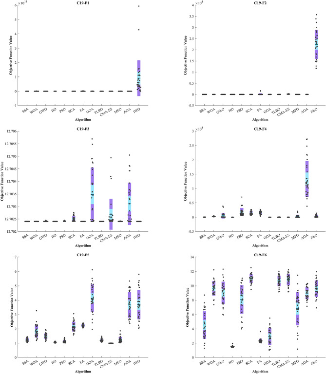
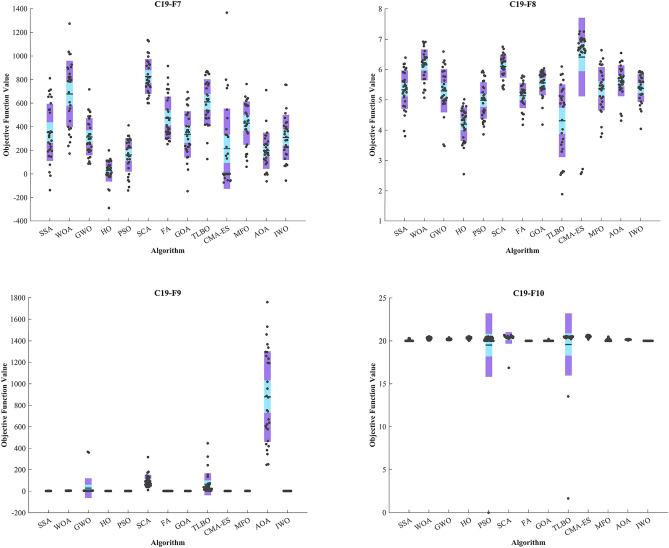
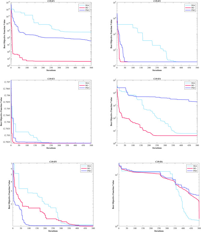
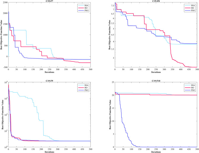
The GOA achieved the top rank in C19-F6. In C19-F7 and C19-F9, it surpassed PSO by a slight margin, and in C19-F8 and C19-F10, it had a slight edge over the TLBO, respectively. Notably, in C19-F7, it outperformed PSO by a considerable margin. Finally, in C19-F8, HO emerged as the best across all criteria except the Best criterion while the TLBO found optimal value of C19-F8. In the box plots of Fig. 9, it is obvious that the HO has a dispersion of almost 0 in C19-F1 to C19-F4. Additionally, C19-F5 and C19-F6 have a much lower Std. than investigated algorithms. In the convergence plots of Fig. 10, we observe the excellent performance of the HO in achieving the optimal solution.
Figure 9.
Boxplot illustrating the performance of the HO in comparison to competing algorithms for optimizing CEC 2019.
Figure 10.
Convergence curves of the top three algorithms in each function in CEC 2019.
Evaluation of the CEC 2014 test suite
The CEC 2014 test suite encompasses a total of 30 standard BFs. These functions are categorized into UM functions (C14–F1 to C14–F3), MM functions with subcategories (C14–F4 to C14–F16), hybrid functions (C14–F17 to C14–F22), and composition functions (C14–F23 to C14–F30)139. The assessment of the HO is documented for CEC 2014 across varying dimensions (10, 30, 50, and 100) by employing 12 different algorithms. The results of this evaluation are presented in Table S1-S3 within the supplementary, accompanied by graphical representations depicted in Fig. S2-S9, illustrating the boxplots and convergence (The top 3 algorithms) diagrams HO has achieved the first rank in 83 out of 120 functions in finding optimal value. In the function (D = 30), C14-F13 had Std. worse than the first rank algorithm with a difference of 0.1 but better than the known GWO, GOA, and CMA-ES algorithms. The same happened in the functions (D = 50) C14-F13 and (D = 100) C14-F5.
In functions (D = 30) C14-F13, (D = 50) C14-F13, and (D = 100) C14-F5 had a slight difference with the first ranking algorithm only in the Std. value. In the function (D = 50), C14-F29 ranked second compared to the PSO algorithm and was not good in Std. and Best compared to the top 3 algorithms. C14–F4 and C14–F30 present ideal choices for assessing the proficiency of metaheuristic algorithms in local search and exploitation due to their absence of local optima. These functions possess a single extremum, prompting a focal objective of assessing the metaheuristic algorithms' efficacy in converging towards the global optimum during optimization endeavours.
Statistical analysis
To thoroughly evaluate the efficacy of the HO, we conduct a comprehensive statistical analysis by comparing it with the reviewed algorithms. The Wilcoxon nonparametric statistical signed-rank test140 checks if there's a big difference between pairs of data (See Table 7) It ranks the differences in size (ignoring whether they are positive or negative) and calculates a number based on those ranks. This number helps determine if the differences are likely due to chance or if they're significant. A small p-value means there's likely a big difference between the paired data. A big p-value means we can't be sure there's a significant difference.
Table 7.
Wilcoxon signed-rank test results.
| Algorithms | Functions | ||||||||
|---|---|---|---|---|---|---|---|---|---|
| Unimodal | High-multimodal | Fixed | CEC 2019 | ZP | CEC 2014 (10) | CEC 2014 (30) | CEC 2014 (50) | CEC 2014 (100) | |
| HO vs. SSA | 1.46E-22 | 2.38E-14 | 4.20E-13 | 4.93E-18 | 8.86E-20 | 4.23E-18 | 3.39E-18 | 4.12E-18 | 7.00E-18 |
| HO vs. WOA | 1.66E-22 | 3.19E-09 | 5.70E-14 | 1.80E-20 | 1.35E-17 | 2.46E-20 | 4.84E-20 | 5.80E-21 | 4.12E-20 |
| HO vs. GWO | 1.34E-21 | 3.09E-06 | 1.17E-13 | 2.27E-19 | 4.89E-18 | 7.82E-19 | 1.08E-19 | 1.17E-19 | 6.35E-19 |
| HO vs. PSO | 1.61E-22 | 9.78E-10 | 4.85E-14 | 6.41E-18 | 3.61E-18 | 1.09E-17 | 3.99E-18 | 3.24E-17 | 8.30E-18 |
| HO vs. SCA | 1.02E-22 | 3.99E-15 | 2.63E-24 | 2.80E-21 | 1.42E-19 | 9.24E-21 | 1.14E-21 | 1.08E-21 | 4.00E-22 |
| HO vs. FA | 8.07E-24 | 2.43E-16 | 1.27E-18 | 6.34E-20 | 2.50E-20 | 2.04E-19 | 1.11E-20 | 4.03E-21 | 5.14E-21 |
| HO vs. GOA | 4.05E-23 | 3.78E-15 | 2.41E-26 | 8.42E-20 | 1.03E-19 | 2.22E-18 | 6.09E-19 | 4.04E-19 | 1.19E-18 |
| HO vs. TLBO | 3.30E-21 | 0.17E-5 | 2.52E-12 | 5.28E-19 | 6.88E-19 | 1.34E-17 | 3.52E-18 | 1.00E-17 | 3.65E-18 |
| HO vs. CMA-ES | 5.64E-24 | 3.74E-17 | 1.10E-12 | 5.78E-20 | 3.84E-21 | 8.70E-18 | 3.14E-19 | 1.06E-20 | 6.30E-21 |
| HO vs. MFO | 5.07E-24 | 6.95E-19 | 1.97E-13 | 4.88E-19 | 6.07E-19 | 2.23E-19 | 7.26E-20 | 3.36E-20 | 1.11E-20 |
| HO vs. AOA | 6.93E-22 | 1.60E-08 | 1.72E-25 | 9.53E-21 | 6.91E-18 | 5.14E-22 | 1.34E-21 | 2.94E-21 | 4.77E-21 |
| HO vs. IWO | 2.85E-23 | 2.57E-15 | 1.31E-17 | 2.20E-20 | 1.08E-20 | 7.73E-20 | 1.03E-19 | 6.96E-20 | 4.36E-20 |
The Friedman test is indeed a non-parametric statistical test used to determine if there are statistically significant differences among multiple related groups (Table 8). This research divided the benchmark functions into seven distinct groups to ensure the test's reliability. The initial group consists of functions delineated in Tables 2, 3, 4, encompassing unimodal, multimodal, and composition functions (F1-F23). The second group comprises the category of ZP functions illustrated in Table 5, while the third group is formed by CEC 2019 functions illustrated in Table 6. The fourth, fifth, sixth, and seventh groups included CEC 2014 functions in different dimensions, respectively (Table S1-S3)141.
Table 8.
Friedman mean rank test results.
| Algorithms | Functions | ||||||
|---|---|---|---|---|---|---|---|
| F1-F23 | ZP | CEC 2019 | CEC 2014 (10) | CEC 2014 (30) | CEC 2014 (50) | CEC 2014 (100) | |
| HO | 2.2468 | 2.0335 | 2.1434 | 2.0226 | 2.0284 | 2.0217 | 2.0256 |
| WOA | 4.693 | 4.966 | 8.5141 | 8.8319 | 7.1239 | 8.434 | 6.8774 |
| GWO | 4.53 | 7.1087 | 7.1867 | 6.9419 | 6.5996 | 7.3247 | 6.0552 |
| SSA | 4.8758 | 9.5542 | 6.2015 | 6.424 | 5.646 | 5.9983 | 6.0104 |
| PSO | 6.3291 | 7.3217 | 4.6159 | 5.8865 | 3.9804 | 3.7454 | 3.9899 |
| SCA | 9.4641 | 8.2399 | 9.4312 | 8.9309 | 9.298 | 9.517 | 9.2506 |
| FA | 10.005 | 9.824 | 7.3172 | 7.3571 | 7.1632 | 8.7833 | 8.1341 |
| GOA | 8.9501 | 8.3386 | 6.9473 | 6.7838 | 5.6549 | 6.3476 | 6.0404 |
| TLBO | 3.8652 | 7.3906 | 6.2127 | 4.2202 | 5.5663 | 5.696 | 6.0148 |
| CMA-ES | 4.4836 | 10.278 | 7.3832 | 6.1895 | 5.7586 | 7.7156 | 7.4959 |
| MFO | 6.9976 | 8.0348 | 7.055 | 7.1332 | 7.0379 | 7.6824 | 7.3757 |
| AOA | 6.3965 | 6.5091 | 8.3732 | 9.1576 | 7.9849 | 9.2846 | 8.2072 |
| IWO | 7.7272 | 9.9419 | 8.303 | 7.7436 | 6.9385 | 7.6078 | 6.2446 |
A post-hoc Nemenyi test was utilized to delve deeper into the distinctions among the algorithms. If the null hypothesis is rejected, a post-hoc test can be conducted. The Nemenyi test is employed when conducting pairwise comparisons among all algorithms. The performance disparity between two classifiers is deemed significant if their respective average ranks exhibit a difference equal to or exceeding the (Eq. 20)141.
| 20 |
represents the number of BFs in each group, represents the number of algorithms under comparison and in each group, we selected the top 10 algorithms for comparison. At a significance level of , the critical value for 10 algorithms, the associated for each group has been specified in Fig. 11. To identify distinctions among the ten algorithms, the derived from the Nemenyi test was employed. The diagrams depicted in Fig. 11 offer straightforward and intuitive visualizations of the outcomes from a Nemenyi post-hoc test. This test is specifically designed to assess the statistical significance of differences in average ranks among a collection of ten algorithms, each evaluated on a set of seven groups.
Figure 11.
Nemenyi test for top ten algorithms in each group with = 0.05.
Following the revelation of notable variations in performance among various algorithms, it becomes imperative to identify which algorithms exhibit significantly different performances compared to HO. HO is regarded as control algorithm in this context. Figure 11 displays the average ranking of each method across seven groups, with significance levels of 0.05 in 30 distinct runs. HO demonstrates significant superiority over algorithms whose average ranking exceeds the threshold line indicated in the figure. In group 1, HO held the first rank in all groups and exhibited significant superiority over TLBO, CMA-ES, GWO, WOA respectively. Moving to group 2, WOA secured the second position after HO and could significantly outperform AOA, GWO, and PSO while in group 3, PSO attained the second position following HO and TLBO, SSA, and GOA are ranked 3, 4, and 5, respectively. In group 4, TLBO outperforms algorithm PSO, and consequently, we observe the placement of algorithms, HO, TLBO, PSO, CMA-ES, SSA but within group 5, the PSO algorithm performs better than the TLBO algorithm. As a result, the arrangement or ranking of algorithms within this group is as follows: HO, PSO, TLBO, GOA, CMA-ES. Continuing, in group 6, it is observable that HO outperforms the other algorithms, and furthermore, the sequence of algorithms is as follows: PSO, TLBO, SSA, GOA, GWO. Lastly in group, the line-up of algorithms is as follows: HO, TLBO, PSO, CMA-ES, SSA.
A post-hoc analysis determines that if the disparity in mean Friedman values between the two algorithms falls below the threshold, there is no notable distinction between them; conversely, if it surpasses the value, a significant difference between the algorithms exists. In Table 9, a comparison has been conducted between 12 algorithms and HO across all seven BF groups. Algorithms that are not significantly different from the HO algorithm are highlighted with a red mark. Conversely, algorithms that are deemed significantly different from the HO algorithm are highlighted with a green mark in this table. In accordance with Table 9, none of the examined algorithms in this article can serve as a substitute for algorithm HO. This observation underscores the necessity of the existence of algorithm HO, which can potentially address limitations not covered by other algorithms.
Table 9.
Nemenyi’s statistical test for seven groups of BFs (Control Algorithm: HO).
| Algorithms | Functions | ||||||
|---|---|---|---|---|---|---|---|
| F1-F23 | ZP | CEC 2019 | CEC 2014 (10) | CEC 2014 (30) | CEC 2014 (50) | CEC 2014 (100) | |
| HO vs. WOA | ❌ | ❌ | ✅ | ✅ | ✅ | ✅ | ✅ |
| HO vs. GWO | ❌ | ✅ | ✅ | ✅ | ✅ | ✅ | ✅ |
| HO vs. SSA | ❌ | ✅ | ❌ | ✅ | ✅ | ✅ | ✅ |
| HO vs. PSO | ✅ | ✅ | ❌ | ✅ | ❌ | ❌ | ❌ |
| HO vs. SCA | ✅ | ✅ | ✅ | ✅ | ✅ | ✅ | ✅ |
| HO vs. FA | ✅ | ✅ | ✅ | ✅ | ✅ | ✅ | ✅ |
| HO vs. GOA | ✅ | ✅ | ✅ | ✅ | ✅ | ✅ | ✅ |
| HO vs. TLBO | ❌ | ✅ | ❌ | ❌ | ✅ | ✅ | ✅ |
| HO vs. CMA-ES | ❌ | ✅ | ✅ | ✅ | ✅ | ✅ | ✅ |
| HO vs. MFO | ✅ | ✅ | ✅ | ✅ | ✅ | ✅ | ✅ |
| HO vs. AOA | ✅ | ❌ | ✅ | ✅ | ✅ | ✅ | ✅ |
| HO vs. IWO | ✅ | ✅ | ✅ | ✅ | ✅ | ✅ | ✅ |
Sensitivity analysis
HO is a swarm-based optimizer that conducts the optimization procedure through iterative calculations. Hence, it is anticipated that the hyperparameters (representing the population size) and (indicating the total number of algorithm iterations) will influence the optimization performance of HO. Consequently, the sensitivity analysis of HO to hyperparameters and is provided in this subsection. To analyze the sensitivity of HO to hyperparameter , the proposed algorithm is employed for different values of , specifically 20, 30, 50, and 100. This variation in is utilized to optimize functions from F1 to F23 BFs.
The optimization results are provided in Table 10, and the convergence curves of HO under this analysis are depicted in Fig. 12. What is evident from the analysis of HO’s sensitivity to the hyperparameter is that increasing the searcher agents improves HO’s search capability in scanning the search space, which enhances the performance of the proposed algorithm and reduces the values of the objective function.
Table 10.
Findings from the sensitivity analysis of HO concerning parameter .
| Objective Functions | Number of population members | |||
|---|---|---|---|---|
| 20 | 30 | 50 | 100 | |
| F1 | 0 | 0 | 0 | 0 |
| F2 | 0 | 0 | 0 | 0 |
| F3 | 0 | 0 | 0 | 0 |
| F4 | 0 | 0 | 0 | 0 |
| F5 | 15.4682 | 2.0125 | 7.0959E-06 | 1.4080E-06 |
| F6 | 0 | 0 | 0 | 0 |
| F7 | 4.3541E-05 | 3.8741E-05 | 2.5178E-05 | 2.1020E-05 |
| F8 | − 9265.3130 | − 9282.0349 | − 9543.2299 | − 9778.5922 |
| F9 | 0 | 0 | 0 | 0 |
| F10 | 4.4409E-16 | 4.4409E-16 | 4.4409E-16 | 4.4409E-16 |
| F11 | 0 | 0 | 0 | 0 |
| F12 | 3.1556E-28 | 1.5705E-32 | 1.5705E-32 | 1.5705E-32 |
| F13 | 1.5802E-24 | 1.3498E-32 | 1.3498E-32 | 1.3498E-32 |
| F14 | 0.9980 | 0.9980 | 0.9980 | 0.9980 |
| F15 | 3.0749E-04 | 3.0749E-04 | 3.0749E-04 | 3.0749E-04 |
| F16 | − 1.0316 | − 1.0316 | − 1.0316 | − 1.0316 |
| F17 | 0.3979 | 0.3979 | 0.3979 | 0.3979 |
| F18 | 3 | 3 | 3 | 3 |
| F19 | − 3.8628 | − 3.8628 | − 3.8628 | − 3.8628 |
| F20 | − 3.3210 | − 3.3220 | − 3.3220 | − 3.3220 |
| F21 | − 10.1532 | − 10.1532 | − 10.1532 | − 10.1532 |
| F22 | − 10.4029 | − 10.4029 | − 10.4029 | − 10.4029 |
| F23 | − 10.5364 | − 10.5364 | − 10.5364 | − 10.5364 |
Figure 12.
The convergence curves of HO during the investigation of sensitivity analysis regarding parameter .
To analyze the sensitivity of the proposed algorithm to hyperparameter , HO is utilized for different values of , specifically 200, 500, 800, and 1000. These variations in are employed to optimize functions from F1 to F23 BFs. The optimization results are provided in Table 11, and the convergence curves of HO under this analysis are depicted in Fig. 13. According results, it is observed that higher values of provide the algorithm with increased opportunities to converge to superior solutions, primarily due to enhanced exploitation ability. Hence, it is evident that as the values of increase, the optimization process becomes more efficient, leading to decreased values of the objective function.
Table 11.
Findings from the sensitivity analysis of HO concerning parameter .
| Objective Functions | Maximum number of iteration | |||
|---|---|---|---|---|
| 200 | 500 | 800 | 1000 | |
| F1 | 0 | 0 | 0 | 0 |
| F2 | 0 | 0 | 0 | 0 |
| F3 | 1.5456E-41 | 0 | 0 | 0 |
| F4 | 1.6531E-66 | 0 | 0 | 0 |
| F5 | 20.9691 | 13.3132 | 5.4924 | 3.3495 |
| F6 | 0 | 0 | 0 | 0 |
| F7 | 2.6782E-04 | 7.1535E-05 | 7.0243E-05 | 1.5269E-05 |
| F8 | − 9.7163E + 03 | − 9.5356E + 03 | − 9.8802E + 03 | − 9.2684E + 03 |
| F9 | 0 | 0 | 0 | 0 |
| F10 | 4.4409E− 16 | 4.4409E-16 | 4.4409E-16 | 4.4409E-16 |
| F11 | 0 | 0 | 0 | 0 |
| F12 | 1.2730E-10 | 3.3597E-24 | 1.5705E-32 | 1.5705E-32 |
| F13 | 3.5137E-08 | 7.2720E-21 | 1.3498E-32 | 1.3498E-32 |
| F14 | 0.9980 | 0.9980 | 0.9980 | 0.9980 |
| F15 | 3.0749E-04 | 3.0749E-04 | 3.0749E-04 | 3.0749E-04 |
| F16 | − 1.0316 | − 1.0316 | − 1.0316 | − 1.0316 |
| F17 | 0.3979 | 0.3979 | 0.3979 | 0.3979 |
| F18 | 3 | 3 | 3 | 3 |
| F19 | − 3.8628 | − 3.8628 | − 3.8628 | − 3.8628 |
| F20 | − 3.3220 | − 3.3220 | − 3.3220 | − 3.3220 |
| F21 | − 10.1532 | − 10.1532 | − 10.1532 | − 10.1532 |
| F22 | − 10.4029 | − 10.4029 | − 10.4029 | − 10.4029 |
| F23 | − 10.5364 | − 10.5364 | − 10.5364 | − 10.5364 |
Figure 13.
The convergence curves of HO during the investigation of sensitivity analysis regarding parameter .
According to Tables 10 which iteration hyperparameter is kept constant and Table 11 which population parameter is held constant, the performance of the HO algorithm improves with an increase in population and iteration, except for F8 as shown in Table 11. Based on the results, it is observed that the algorithm is less sensitive to changes in the iteration hyperparameter (Table 12).
Table 12.
The attributes of the wind turbine.
| Parameter | Value |
|---|---|
| Thrust coefficient () | 0.88 |
| Ground surface roughness () | 0.3 |
| Hub height () | 60 m |
| Rotor diameter () | 40 m |
| Turbine efficiency ( ) | 40% |
| Air density () | 1.225 kg/m3 |
| Wind speed () | 12 m/s |
| Wind directions (degree) |
{10°, 20°, 30°,…,360°} wind direction angle w.r.t. + x (East) |
Hippopotamus optimization algorithm for engineering problems
In this section, the effectiveness of the HO is evaluated in relation to its ability to address practical optimization problems in four of problem distinct engineering design challenges. The HO is employed to solve these problems, utilizing a total of 30,000 evaluations. The statistical outcomes obtained using various methodologies are showcased in Table 13. Additionally, Fig. 18 illustrates the boxplots of the algorithms.
Table 13.
Evaluation results of the engineering problems.
| F | M | Optimization Algorithms | ||||||||||||
|---|---|---|---|---|---|---|---|---|---|---|---|---|---|---|
| HO | WOA | GWO | SSA | PSO | SCA | FA | GOA | TLBO | CMA-ES | MFO | AOA | IWO | ||
| TCS | Mean | 0.012665 | 0.013544 | 0.012769 | 0.013057 | 0.013759 | 0.013033 | 0.01277 | 0.62228 | 0.012677 | 0.013488 | 0.013466 | 0.017608 | 0.012829 |
| Best | 0.012665 | 0.012675 | 0.012672 | 0.012669 | 0.012667 | 0.012728 | 0.012666 | 0.013193 | 0.012665 | 0.012665 | 0.012667 | 0.013195 | 0.012713 | |
| Worst | 0.012665 | 0.016002 | 0.013689 | 0.015436 | 0.016642 | 0.013222 | 0.01311 | 2.7935 | 0.012703 | 0.017773 | 0.017773 | 0.034425 | 0.014 | |
| Std | 2.95E-09 | 0.0010105 | 0.00019007 | 0.00065595 | 0.0011223 | 0.00014162 | 0.0001116 | 1.0199 | 9.61E-06 | 0.0012441 | 0.001263 | 0.0080586 | 0.0002798 | |
| Median | 0.012665 | 0.013124 | 0.012722 | 0.012824 | 0.013348 | 0.013033 | 0.012719 | 0.050421 | 0.012676 | 0.012973 | 0.013193 | 0.013261 | 0.012747 | |
| Rank | 1 | 10 | 3 | 7 | 11 | 6 | 4 | 13 | 2 | 9 | 8 | 12 | 5 | |
| PV | Mean | 6102.7 | 7217.2 | 6976 | 6304.6 | 6327.7 | 6718.2 | 6294.4 | 7817.5 | 12,292 | 6534.1 | 6587.4 | 6471.7 | 8758.1 |
| Best | 6059.7 | 6149.7 | 6069.6 | 6059.7 | 6059.7 | 6173.7 | 6059.7 | 6059.7 | 6069.6 | 6059.7 | 6059.7 | 6059.7 | 6540.5 | |
| Worst | 7306.6 | 7857.6 | 10,069 | 6820.4 | 7047.3 | 7690.7 | 7306.5 | 17,459 | 34,344 | 7368.1 | 7682.9 | 7306.9 | 11,672 | |
| Std | 227.45 | 592.21 | 915.11 | 244.96 | 262.97 | 476.06 | 386.97 | 2691.5 | 6840.1 | 524.75 | 592.82 | 436.61 | 1704.9 | |
| Median | 6059.7 | 7596.2 | 7307.6 | 6237.2 | 6315.8 | 6503.8 | 6090.5 | 6523.2 | 10,020 | 6315.9 | 6317.1 | 6363 | 8520.7 | |
| Rank | 1 | 10 | 9 | 3 | 4 | 8 | 2 | 11 | 13 | 6 | 7 | 5 | 12 | |
| WB | Mean | 1.7249 | 2.7799 | 1.7273 | 1.8772 | 1.7249 | 1.87 | 1.7249 | 3.9995 | 1.7249 | 1.7934 | 1.7768 | 2.4201 | 1.9001 |
| Best | 1.7249 | 1.821 | 1.7254 | 1.7296 | 1.7249 | 1.7794 | 1.7249 | 1.9706 | 1.7249 | 1.7249 | 1.7249 | 2.0184 | 1.7268 | |
| Worst | 1.7249 | 6.0369 | 1.7359 | 2.1965 | 1.7249 | 1.9655 | 1.7249 | 5.9584 | 1.7249 | 2.3189 | 2.3788 | 2.7457 | 2.2028 | |
| Std | 1.16E-15 | 1.1889 | 0.0022462 | 0.14429 | 4.57E-09 | 0.036549 | 8.13E-08 | 1.0734 | 9.12E-16 | 0.13205 | 0.15727 | 0.14915 | 0.2014 | |
| Median | 1.7249 | 2.1722 | 1.7266 | 1.8146 | 1.7249 | 1.8729 | 1.7249 | 3.8978 | 1.7249 | 1.732 | 1.7252 | 2.4641 | 1.7552 | |
| Rank | 1 | 9 | 2 | 6 | 1 | 5 | 1 | 10 | 1 | 4 | 3 | 8 | 7 | |
| WFLO | Mean | 0.0014571 | 0.0014576 | 0.0014672 | 0.0014678 | 0.0014621 | 0.0014644 | 0.0014581 | 0.0014662 | 0.0014735 | 0.0014689 | 0.0014752 | 0.0014635 | 0.0014638 |
| Best | 0.0014557 | 0.0014565 | 0.0014638 | 0.0014653 | 0.0014595 | 0.0014608 | 0.0014567 | 0.0014622 | 0.0014669 | 0.0014612 | 0.0014683 | 0.0014583 | 0.0014581 | |
| Worst | 0.0014596 | 0.0014593 | 0.0014692 | 0.0014702 | 0.0014662 | 0.0014671 | 0.0014616 | 0.0014686 | 0.001478 | 0.0014793 | 0.0014807 | 0.0014697 | 0.0014705 | |
| Std | 6.39E-07 | 1.44E-06 | 1.19E-06 | 1.08E-06 | 1.80E-06 | 1.64E-06 | 1.10E-06 | 1.94E-06 | 2.64E-06 | 4.78E-06 | 3.82E-06 | 2.58E-06 | 3.40E-06 | |
| Median | 0.0014563 | 0.0014575 | 0.0014673 | 0.0014683 | 0.0014621 | 0.0014647 | 0.0014579 | 0.0014671 | 0.0014738 | 0.0014689 | 0.0014758 | 0.0014633 | 0.0014638 | |
| Rank | 1 | 2 | 9 | 10 | 4 | 7 | 3 | 8 | 12 | 11 | 13 | 5 | 6 | |
Figure 18.
Boxplot illustrating the performance of the HO in comparison to twelve algorithms for optimizing TCS, WB, PV and WFLO.
TCS design
This problem's primary aim entails minimizing the mass associated with the spring, as illustrated in Fig. 14, considering whether it is stretched or compressed. In order to achieve optimal design, it is important to ensure wave frequency, deflection limits, and stress are met. The mathematical representation of this engineering design can be described by the equation in Supplementary142. Based on the obtained outcomes, the HO has successfully obtained the optimal solution. Simultaneously, it ensures compliance with the specified constraints, as detailed in the references45,102,142–145. The optimal solutions achieved through the utilization of HO for this particular problem are {}.
Figure 14.
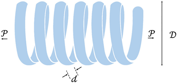
TCS.
WB design
The objective is to minimize the cost associated with the welding beam. This objective is achieved by simultaneously addressing seven constraints. The problem concerning the design of a welded beam is visually depicted in Fig. 15. The optimal design problem for the welded beam is formulated as described in Supplementary49. The HO has the capability to identify the most favourable value for the optimization variables. Statistical analysis determined that that the HO exhibits superior performance. The optimal solutions achieved through the utilization of HO for this particular problem are {}.
Figure 15.
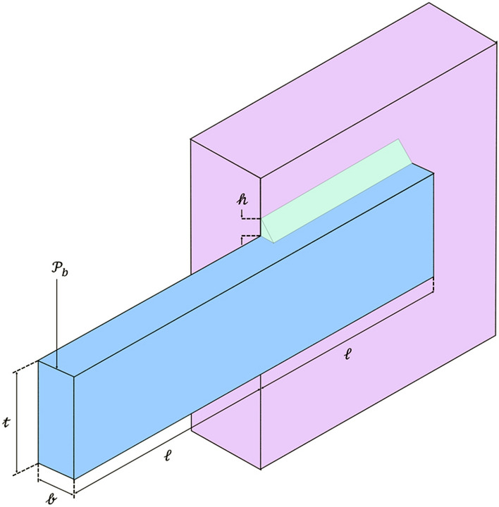
WB.
PV design
The primary objective revolves around minimizing the overall cost associated with the tank under pressurized conditions, considering factors such as forming techniques, welding methods, and material costs, as depicted in Fig. 16. The design process involves considering four variables and four constraints. The PV design problem is formulated as described in Supplementary49 .According to the reported results, the HO outperformed other methods. The optimal solutions achieved through the utilization of HO for this particular problem are {}. Further details regarding these constraints can be found in references69 and145.
Figure 16.
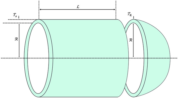
PV.
WFLO
We're figuring out where to place wind turbines on a 10 10 grid. We have 100 different options for where to put the turbines. We can have anywhere from 1 to 39 turbines in the wind farm. We're simulating wind coming from 36 different directions, all at a steady speed of 12 m per second. The objective is to minimize expenditures, maximize the aggregate power output, reduce acoustic emissions, and optimize various performance and cost-related metrics13 (Fig. 17). The attributes of the wind turbine are documented in Table 12. The formulation of WFLO problem is articulated as follows:
| 21 |
Figure 17.
WFLO with HO.
Herein, represents a vector comprising design variables, while denotes the aggregate power output generated by a wind farm. The computation of the function can be derived according to the method described in146 (Fig. 18).
| 22 |
The HO demonstrating superior performance compared to alternative approaches.
Ethical approval
This article does not contain any studies with human participants or animals performed by any of the authors. Informed consent was not required as no human or animals were involved.
Conclusions and future works
In this paper, we introduced a novel nonparametric optimization algorithm called the Hippopotamus Optimization (HO). The real inspiration behind the HO is to simulate the behaviors of hippopotamuses, incorporating their spatial positioning in the water, defense strategies against threats, and evasion techniques from predators. The algorithm is outlined conceptually through a trinary-phase model of their position update in river and pound, defense, and evading predators, each mathematically defined. In light of the results from addressing four distinct engineering design challenges, the HO has effectively achieved the most efficient resolution while concurrently upholding adherence to the designated constraints. The acquired outcomes from the HO were compared with the performance of 12 established metaheuristic algorithms. The algorithm achieved the highest ranking across 115 out of 161 BFs in finding optimal value. These benchmarks span various function types, including UM and HM functions, FM functions, in addition to the CEC 2019 test suite and CEC 2014 dimensions encompassing 10, 30, 50, and 100, along with the ZP.
The results of CEC 2014 test suite indicate that the HO swiftly identifies optimal solutions, avoiding entrapment in local minima. It consistently pursues highly optimal solutions at an impressive pace by employing efficient local search strategies. Furthermore, upon evaluation using the CEC 2019 test, it can be confidently asserted that the HO effectively finds the global optimal solution. Additionally, in the ZP, the HO demonstrates significantly superior performance compared to its competitors, achieving an optimal solution that remains unattainable for other investigated algorithms. Moreover, the observed lower Std. than that of the other investigated algorithms suggests that the HO displays resilience and efficacy in effectively addressing these functions.
Considering the outcomes derived from tackling four unique engineering design challenges, the HO has effectively demonstrated the most efficient resolution while maintaining strict adherence to the specified constraints. The application of the Wilcoxon signed test, Friedman and Nemenyi post-hoc test confirms that the HO displays a remarkable and statistically significant advantage over the algorithms under investigation in effectively addressing the optimization problems scrutinized in this study. The findings indicate that Ho exhibits lower sensitivity to changes in the iteration hyperparameter than the population hyperparameter.
The suggested methodology, HO, presents numerous avenues for future research exploration. Particularly, an area ripe with potential is the advancement of binary and multi-objective variants based on this proposed methodology. Furthermore, an avenue worth investigating in forthcoming research involves employing HO in optimizing diverse problem sets across multiple domains and real-world contexts.
Supplementary Information
Abbreviations
- MaxIter
Max number of iterations
- BF
Benchmark Function
- UM
Unimodal
- MM
Multimodal
- FM
Fixed-dimension Multimodal
- HM
High-dimensional Multimodal
- ZP
Zigzag Pattern benchmark test
- TCS
Tension/Compression Spring
- WB
Welded Beam
- PV
Pressure Vessel
- WFLO
Wind Farm Layout Optimization
- F
Function
- CEC
IEEE Congress on Evolutionary Computation
- D
Dimension
- C19
CEC2019
- C14
CEC2014
- CMA-ES
Evolution Strategy with Covariance Matrix Adaptation
- MFO
Moth-flame Optimization
- AOA
Arithmetic Optimization Algorithm
- TLBO
Teaching-Learning-Based Optimization
- IWO
Invasive Weed Optimization
- GOA
Grasshopper Optimization Algorithm
- FA
Firefly Algorithm
- PSO
Particle Swarm Optimization
- SSA
Salp Swarm Algorithm
- CD
Critical Difference
- GWO
Gray Wolf Optimization
- SCA
Sine Cosine Algorithm
- WOA
Whale Optimization Algorithm
- Best
The best result
- Worst
The worst result
- Std.
Standard Deviation
- Mean
Average best result
Author contributions
Conceptualization, M.H.A. and N.M.H., methodology, M.H.A. and N.M.H., software, M.H.A. and N.M.H., validation, M.H.A. and N.M.H., formal analysis, M.H.A. and N.M.H., investigation, M.H.A. and N.M.H., resources, M.H.A. and N.M.H., data curation, M.H.A. and N.M.H., writing original draft preparation, M.H.A. and N.M.H., writing review and editing, M.H.A. and N.M.H., visualization, M.M., N.K. and S.M., supervision, M.H.A. and N.M.H., project administration.
Data availability
All data generated or analyzed during this study are included directly in the text of this submitted manuscript. There are no additional external files with datasets.
Competing interests
The authors declare no competing interests.
Footnotes
Publisher's note
Springer Nature remains neutral with regard to jurisdictional claims in published maps and institutional affiliations.
Supplementary Information
The online version contains supplementary material available at 10.1038/s41598-024-54910-3.
References
- 1.Dhiman G, Garg M, Nagar A, Kumar V, Dehghani M. A novel algorithm for global optimization: Rat swarm optimizer. J. Ambient Intell. Humaniz Comput. 2021;12:8457–8482. doi: 10.1007/s12652-020-02580-0. [DOI] [Google Scholar]
- 2.Chen H, et al. An opposition-based sine cosine approach with local search for parameter estimation of photovoltaic models. Energy Convers Manag. 2019;195:927–942. doi: 10.1016/j.enconman.2019.05.057. [DOI] [Google Scholar]
- 3.Li S, Chen H, Wang M, Heidari AA, Mirjalili S. Slime mould algorithm: A new method for stochastic optimization. Futur. Gener. Comput. Syst. 2020;111:300–323. doi: 10.1016/j.future.2020.03.055. [DOI] [Google Scholar]
- 4.Gharaei A, Shekarabi S, Karimi M. Modelling and optimal lot-sizing of the replenishments in constrained, multi-product and bi-objective EPQ models with defective products: Generalised cross decomposition. Int. J. Syst. Sci. 2019 doi: 10.1080/23302674.2019.1574364. [DOI] [Google Scholar]
- 5.Sayadi R, Awasthi A. An integrated approach based on system dynamics and ANP for evaluating sustainable transportation policies. Int. J. Syst. Sci.: Op. Logist. 2018;7:1–10. [Google Scholar]
- 6.Golalipour K, et al. The corona virus search optimizer for solving global and engineering optimization problems. Alex. Eng. J. 2023;78:614–642. doi: 10.1016/j.aej.2023.07.066. [DOI] [Google Scholar]
- 7.Wolpert DH, Macready WG. No free lunch theorems for optimization. IEEE Trans. Evolut. Comput. 1997;1:67–82. doi: 10.1109/4235.585893. [DOI] [Google Scholar]
- 8.Emam MM, Samee NA, Jamjoom MM, Houssein EH. Optimized deep learning architecture for brain tumor classification using improved hunger games search algorithm. Comput. Biol. Med. 2023;160:106966. doi: 10.1016/j.compbiomed.2023.106966. [DOI] [PubMed] [Google Scholar]
- 9.Lu D, et al. Effective detection of Alzheimer’s disease by optimizing fuzzy K-nearest neighbors based on salp swarm algorithm. Comput. Biol. Med. 2023;159:106930. doi: 10.1016/j.compbiomed.2023.106930. [DOI] [PubMed] [Google Scholar]
- 10.Patel HR, Shah VA. Fuzzy Logic Based Metaheuristic Algorithm for Optimization of Type-1 Fuzzy Controller: Fault-Tolerant Control for Nonlinear System with Actuator Fault⁎⁎The author(s) received funding for the ACODS-2022 registration fees from Dharmsinh Desai University, Nadiad-387001, Gujarat, India. IFAC-PapersOnLine. 2022;55:715–721. doi: 10.1016/j.ifacol.2022.04.117. [DOI] [Google Scholar]
- 11.Ekinci S, Izci D. Enhancing IIR system identification: Harnessing the synergy of gazelle optimization and simulated annealing algorithms. ePrime – Adv. Electr. Eng.Electron. Energy. 2023;5:100225. doi: 10.1016/j.prime.2023.100225. [DOI] [Google Scholar]
- 12.Refaat A, et al. A novel metaheuristic MPPT technique based on enhanced autonomous group particle swarm optimization algorithm to track the GMPP under partial shading conditions - Experimental validation. Energy Convers Manag. 2023;287:117124. doi: 10.1016/j.enconman.2023.117124. [DOI] [Google Scholar]
- 13.Kunakote T, et al. Comparative performance of twelve metaheuristics for wind farm layout optimisation. Archiv. Comput. Methods Eng. 2022;29:717–730. doi: 10.1007/s11831-021-09586-7. [DOI] [Google Scholar]
- 14.Ocak A, Melih Nigdeli S, Bekdaş G. Optimization of the base isolator systems by considering the soil-structure interaction via metaheuristic algorithms. Structures. 2023;56:104886. doi: 10.1016/j.istruc.2023.104886. [DOI] [Google Scholar]
- 15.Domínguez A, Juan A, Kizys R. A survey on financial applications of metaheuristics. ACM Comput. Surv. 2017;50:1–23. doi: 10.1145/3054133. [DOI] [Google Scholar]
- 16.Han S, et al. Thermal-economic optimization design of shell and tube heat exchanger using an improved sparrow search algorithm. Therm. Sci. Eng. Progress. 2023;45:102085. doi: 10.1016/j.tsep.2023.102085. [DOI] [Google Scholar]
- 17.Hazra A, Rana P, Adhikari M, Amgoth T. Fog computing for next-generation Internet of Things: Fundamental, state-of-the-art and research challenges. Comput. Sci. Rev. 2023;48:100549. doi: 10.1016/j.cosrev.2023.100549. [DOI] [Google Scholar]
- 18.Mohapatra S, Mohapatra P. American zebra optimization algorithm for global optimization problems. Sci. Rep. 2023;13:5211. doi: 10.1038/s41598-023-31876-2. [DOI] [PMC free article] [PubMed] [Google Scholar]
- 19.Dehghani M, Hubálovský Š, Trojovský P. Northern goshawk optimization: A new swarm-based algorithm for solving optimization problems. IEEE Access. 2021;9:162059–162080. doi: 10.1109/ACCESS.2021.3133286. [DOI] [Google Scholar]
- 20.Kennedy, J. & Eberhart, R. Particle swarm optimization. in Proceedings of ICNN’95 - International Conference on Neural Networks vol. 4 1942–1948 (1995).
- 21.Dorigo M, Birattari M, Stutzle T. Ant colony optimization. IEEE Comput. Intell. Mag. 2006;1:28–39. doi: 10.1109/MCI.2006.329691. [DOI] [Google Scholar]
- 22.Kang F, Li J, Ma Z. Rosenbrock artificial bee colony algorithm for accurate global optimization of numerical functions. Inf. Sci. 2011;181:3508–3531. doi: 10.1016/j.ins.2011.04.024. [DOI] [Google Scholar]
- 23.Kaur S, Awasthi LK, Sangal AL, Dhiman G. Tunicate Swarm Algorithm: A new bio-inspired based metaheuristic paradigm for global optimization. Eng. Appl. Artif. Intell. 2020;90:103541. doi: 10.1016/j.engappai.2020.103541. [DOI] [Google Scholar]
- 24.Zhong C, Li G, Meng Z. Beluga whale optimization: A novel nature-inspired metaheuristic algorithm. Knowl. Based Syst. 2022;251:109215. doi: 10.1016/j.knosys.2022.109215. [DOI] [Google Scholar]
- 25.Eslami N, Yazdani S, Mirzaei M, Hadavandi E. Aphid-Ant Mutualism: A novel nature-inspired metaheuristic algorithm for solving optimization problems. Math. Comput. Simul. 2022;201:362–395. doi: 10.1016/j.matcom.2022.05.015. [DOI] [Google Scholar]
- 26.Chou J-S, Truong D-N. A novel metaheuristic optimizer inspired by behavior of jellyfish in ocean. Appl Math Comput. 2021;389:125535. doi: 10.1016/j.amc.2020.125535. [DOI] [Google Scholar]
- 27.Dhiman G, Kumar V. Spotted hyena optimizer: A novel bio-inspired based metaheuristic technique for engineering applications. Adv. Eng. Softw. 2017;114:48–70. doi: 10.1016/j.advengsoft.2017.05.014. [DOI] [Google Scholar]
- 28.Hashim FA, Houssein EH, Hussain K, Mabrouk MS, Al-Atabany W. Honey badger algorithm: New metaheuristic algorithm for solving optimization problems. Math. Comput. Simul. 2022;192:84–110. doi: 10.1016/j.matcom.2021.08.013. [DOI] [Google Scholar]
- 29.Abdel-Basset M, Mohamed R, Zidan M, Jameel M, Abouhawwash M. Mantis search algorithm: A novel bio-inspired algorithm for global optimization and engineering design problems. Comput. Methods Appl. Mech. Eng. 2023;415:116200. doi: 10.1016/j.cma.2023.116200. [DOI] [Google Scholar]
- 30.Abdel-Basset M, Mohamed R, Jameel M, Abouhawwash M. Nutcracker optimizer: A novel nature-inspired metaheuristic algorithm for global optimization and engineering design problems. Knowl. Based Syst. 2023;262:110248. doi: 10.1016/j.knosys.2022.110248. [DOI] [Google Scholar]
- 31.Zhao W, Zhang Z, Wang L. Manta ray foraging optimization: An effective bio-inspired optimizer for engineering applications. Eng. Appl. Artif. Intell. 2020;87:103300. doi: 10.1016/j.engappai.2019.103300. [DOI] [Google Scholar]
- 32.Jiang Y, Wu Q, Zhu S, Zhang L. Orca predation algorithm: A novel bio-inspired algorithm for global optimization problems. Expert Syst. Appl. 2022;188:116026. doi: 10.1016/j.eswa.2021.116026. [DOI] [Google Scholar]
- 33.Zaldívar D, et al. A novel bio-inspired optimization model based on Yellow Saddle Goatfish behavior. Biosystems. 2018;174:1–21. doi: 10.1016/j.biosystems.2018.09.007. [DOI] [PubMed] [Google Scholar]
- 34.Guo J, et al. A novel hermit crab optimization algorithm. Sci. Rep. 2023;13:9934. doi: 10.1038/s41598-023-37129-6. [DOI] [PMC free article] [PubMed] [Google Scholar]
- 35.Akbari MA, Zare M, Azizipanah-abarghooee R, Mirjalili S, Deriche M. The cheetah optimizer: A nature-inspired metaheuristic algorithm for large-scale optimization problems. Sci. Rep. 2022;12:10953. doi: 10.1038/s41598-022-14338-z. [DOI] [PMC free article] [PubMed] [Google Scholar]
- 36.Trojovský P, Dehghani M. A new bio-inspired metaheuristic algorithm for solving optimization problems based on walruses behavior. Sci. Rep. 2023;13:8775. doi: 10.1038/s41598-023-35863-5. [DOI] [PMC free article] [PubMed] [Google Scholar]
- 37.Ferahtia S, et al. Red-tailed hawk algorithm for numerical optimization and real-world problems. Sci. Rep. 2023;13:12950. doi: 10.1038/s41598-023-38778-3. [DOI] [PMC free article] [PubMed] [Google Scholar]
- 38.Ai H, et al. Magnetic anomaly inversion through the novel barnacles mating optimization algorithm. Sci. Rep. 2022;12:22578. doi: 10.1038/s41598-022-26265-0. [DOI] [PMC free article] [PubMed] [Google Scholar]
- 39.Xian S, Feng X. Meerkat optimization algorithm: A new meta-heuristic optimization algorithm for solving constrained engineering problems. Expert Syst. Appl. 2023;231:120482. doi: 10.1016/j.eswa.2023.120482. [DOI] [Google Scholar]
- 40.Hashim FA, Hussien AG. Snake optimizer: A novel meta-heuristic optimization algorithm. Knowl. Based Syst. 2022;242:108320. doi: 10.1016/j.knosys.2022.108320. [DOI] [Google Scholar]
- 41.Saremi S, Mirjalili S, Lewis A. Grasshopper optimisation algorithm: Theory and application. Adv. Eng. Softw. 2017;105:30–47. doi: 10.1016/j.advengsoft.2017.01.004. [DOI] [Google Scholar]
- 42.Yu JJQ, Li VOK. A social spider algorithm for global optimization. Appl. Soft Comput. 2015;30:614–627. doi: 10.1016/j.asoc.2015.02.014. [DOI] [Google Scholar]
- 43.Mirjalili S, Lewis A. The whale optimization algorithm. Adv. Eng. Softw. 2016;95:51–67. doi: 10.1016/j.advengsoft.2016.01.008. [DOI] [Google Scholar]
- 44.Mirjalili S. The ant lion optimizer. Adv. Eng. Softw. 2015;83:80–98. doi: 10.1016/j.advengsoft.2015.01.010. [DOI] [Google Scholar]
- 45.Mirjalili S, Mirjalili SM, Lewis A. Grey wolf optimizer. Adv. Eng. Softw. 2014;69:46–61. doi: 10.1016/j.advengsoft.2013.12.007. [DOI] [Google Scholar]
- 46.Faramarzi A, Heidarinejad M, Mirjalili S, Gandomi AH. Marine predators algorithm: A nature-inspired metaheuristic. Expert Syst. Appl. 2020;152:113377. doi: 10.1016/j.eswa.2020.113377. [DOI] [Google Scholar]
- 47.Abualigah L, et al. Aquila Optimizer: A novel meta-heuristic optimization algorithm. Comput Ind Eng. 2021;157:107250. doi: 10.1016/j.cie.2021.107250. [DOI] [Google Scholar]
- 48.Abdollahzadeh B, Gharehchopogh FS, Khodadadi N, Mirjalili S. Mountain gazelle optimizer: A new nature-inspired metaheuristic algorithm for global optimization problems. Adv. Eng. Softw. 2022;174:103282. doi: 10.1016/j.advengsoft.2022.103282. [DOI] [Google Scholar]
- 49.Zhao W, Wang L, Mirjalili S. Artificial hummingbird algorithm: A new bio-inspired optimizer with its engineering applications. Comput. Methods Appl. Mech. Eng. 2022;388:114194. doi: 10.1016/j.cma.2021.114194. [DOI] [Google Scholar]
- 50.Abdollahzadeh B, Gharehchopogh FS, Mirjalili S. African vultures optimization algorithm: A new nature-inspired metaheuristic algorithm for global optimization problems. Comput. Ind. Eng. 2021;158:107408. doi: 10.1016/j.cie.2021.107408. [DOI] [Google Scholar]
- 51.Das AK, Pratihar DK. Bonobo optimizer (BO): An intelligent heuristic with self-adjusting parameters over continuous spaces and its applications to engineering problems. Appl. Intell. 2022;52:2942–2974. doi: 10.1007/s10489-021-02444-w. [DOI] [Google Scholar]
- 52.Mirjalili S, et al. Salp swarm algorithm: A bio-inspired optimizer for engineering design problems. Adv. Eng. Softw. 2017;114:163–191. doi: 10.1016/j.advengsoft.2017.07.002. [DOI] [Google Scholar]
- 53.Heidari AA, et al. Harris hawks optimization: Algorithm and applications. Futur. Gener. Comput. Syst. 2019;97:849–872. doi: 10.1016/j.future.2019.02.028. [DOI] [Google Scholar]
- 54.Tu J, Chen H, Wang M, Gandomi AH. The colony predation algorithm. J. Bionic. Eng. 2021;18:674–710. doi: 10.1007/s42235-021-0050-y. [DOI] [Google Scholar]
- 55.ALRahhal H, Jamous R. AFOX: A new adaptive nature-inspired optimization algorithm. Artif. Intell. Rev. 2023 doi: 10.1007/s10462-023-10542-z. [DOI] [Google Scholar]
- 56.Abdel-Basset M, Mohamed R, Jameel M, Abouhawwash M. Spider wasp optimizer: A novel meta-heuristic optimization algorithm. Artif. Intell. Rev. 2023;56:11675–11738. doi: 10.1007/s10462-023-10446-y. [DOI] [Google Scholar]
- 57.Abdollahzadeh B, Soleimanian Gharehchopogh F, Mirjalili S. Artificial gorilla troops optimizer: A new nature-inspired metaheuristic algorithm for global optimization problems. Int. J. Intell. Syst. 2021;36:5887–5958. doi: 10.1002/int.22535. [DOI] [Google Scholar]
- 58.Gandomi AH, Alavi AH. Krill herd: A new bio-inspired optimization algorithm. Commun. Nonlinear Sci. Numer. Simul. 2012;17:4831–4845. doi: 10.1016/j.cnsns.2012.05.010. [DOI] [Google Scholar]
- 59.Yuan Y, et al. Alpine skiing optimization: A new bio-inspired optimization algorithm. Adv. Eng. Softw. 2022;170:103158. doi: 10.1016/j.advengsoft.2022.103158. [DOI] [Google Scholar]
- 60.Eusuff M, Lansey K, Pasha F. Shuffled frog-leaping algorithm: A memetic meta-heuristic for discrete optimization. Eng. Optimiz. 2006;38:129–154. doi: 10.1080/03052150500384759. [DOI] [Google Scholar]
- 61.Yang X-S. Chapter 8 - Firefly Algorithms. In: Yang X-S, editor. Nature-Inspired Optimization Algorithms. Elsevier; 2014. pp. 111–127. [Google Scholar]
- 62.Suyanto S, Ariyanto AA, Ariyanto AF. Komodo Mlipir Algorithm. Appl. Soft Comput. 2022;114:108043. doi: 10.1016/j.asoc.2021.108043. [DOI] [Google Scholar]
- 63.Ezugwu AE, Agushaka JO, Abualigah L, Mirjalili S, Gandomi AH. Prairie dog optimization algorithm. Neural Comput. Appl. 2022;34:20017–20065. doi: 10.1007/s00521-022-07530-9. [DOI] [PMC free article] [PubMed] [Google Scholar]
- 64.Dehghani M, Hubálovský Š, Trojovský P. Tasmanian devil optimization: A new bio-inspired optimization algorithm for solving optimization algorithm. IEEE Access. 2022;10:19599–19620. doi: 10.1109/ACCESS.2022.3151641. [DOI] [Google Scholar]
- 65.Abualigah L, Elaziz MA, Sumari P, Geem ZW, Gandomi AH. Reptile search algorithm (RSA): A nature-inspired meta-heuristic optimizer. Expert Syst. Appl. 2022;191:116158. doi: 10.1016/j.eswa.2021.116158. [DOI] [Google Scholar]
- 66.Dutta T, Bhattacharyya S, Dey S, Platos J. Border collie optimization. IEEE Access. 2020;8:109177–109197. doi: 10.1109/ACCESS.2020.2999540. [DOI] [Google Scholar]
- 67.Saba J, Bozorg-Haddad O, Cuckoo CX. Cuckoo optimization algorithm (COA) In: Bozorg-Haddad O, editor. Advanced Optimization by Nature-Inspired Algorithms. Springer Singapore; 2018. pp. 39–49. [Google Scholar]
- 68.Mirjalili S. Moth-flame optimization algorithm: A novel nature-inspired heuristic paradigm. Knowl. Based Syst. 2015;89:228–249. doi: 10.1016/j.knosys.2015.07.006. [DOI] [Google Scholar]
- 69.Whitley, D. A Genetic Algorithm Tutorial. Stat Comput4, (1998).
- 70.Moscato, P. On Evolution, Search, Optimization, Genetic Algorithms and Martial Arts: Towards Memetic Algorithms. (1989).
- 71.Storn R, Price K. Differential evolution – a simple and efficient heuristic for global optimization over continuous spaces. J. Global Optimiz. 1997;11:341–359. doi: 10.1023/A:1008202821328. [DOI] [Google Scholar]
- 72.Beyer H-G, Schwefel H-P. Evolution strategies–a comprehensive introduction. Nat. Comput. 2002;1:3–52. doi: 10.1023/A:1015059928466. [DOI] [Google Scholar]
- 73.Simon D. Biogeography-based optimization. IEEE Trans. Evolut. Comput. 2008;12:702–713. doi: 10.1109/TEVC.2008.919004. [DOI] [Google Scholar]
- 74.Houssein EH, Oliva D, Samee NA, Mahmoud NF, Emam MM. Liver cancer algorithm: A novel bio-inspired optimizer. Comput. Biol. Med. 2023 doi: 10.1016/j.compbiomed.2023.107389. [DOI] [PubMed] [Google Scholar]
- 75.Banzhaf W, Francone FD, Keller RE, Nordin P. Genetic Programming: An Introduction: On the Automatic Evolution of Computer Programs and Its Applications. Morgan Kaufmann Publishers Inc.; 1998. [Google Scholar]
- 76.Xing B, Gao W-J. Invasive Weed Optimization Algorithm. In: Xing B, Gao W-J, editors. Innovative Computational Intelligence: A Rough Guide to 134 Clever Algorithms. Springer International Publishing; 2014. pp. 177–181sZ. [Google Scholar]
- 77.Zhao W, et al. Electric eel foraging optimization: A new bio-inspired optimizer for engineering applications. Expert Syst. Appl. 2024;238:122200. doi: 10.1016/j.eswa.2023.122200. [DOI] [Google Scholar]
- 78.El-kenawy ESM, et al. Greylag goose optimization: Nature-inspired optimization algorithm. Expert Syst Appl. 2024;238:122147. doi: 10.1016/j.eswa.2023.122147. [DOI] [Google Scholar]
- 79.Abdollahzadeh B, et al. Puma optimizer (PO): A novel metaheuristic optimization algorithm and its application in machine learning. Cluster Comput. 2024 doi: 10.1007/S10586-023-04221-5/TABLES/28. [DOI] [Google Scholar]
- 80.Cheng R, Jin Y. A competitive swarm optimizer for large scale optimization. IEEE Trans. Cybern. 2015;45:191–204. doi: 10.1109/TCYB.2014.2322602. [DOI] [PubMed] [Google Scholar]
- 81.de Vasconcelos Segundo EH, Mariani VC, dos Coelho LS. Design of heat exchangers using Falcon Optimization Algorithm. Appl. Therm. Eng. 2019;156:119–144. doi: 10.1016/j.applthermaleng.2019.04.038. [DOI] [Google Scholar]
- 82.Sulaiman MH, Mustaffa Z, Saari MM, Daniyal H. Barnacles mating optimizer: A new bio-inspired algorithm for solving engineering optimization problems. Eng. Appl. Artif. Intell. 2020;87:103330. doi: 10.1016/j.engappai.2019.103330. [DOI] [Google Scholar]
- 83.Yapici H, Cetinkaya N. A new meta-heuristic optimizer: Pathfinder algorithm. Appl. Soft Comput. 2019;78:545–568. doi: 10.1016/j.asoc.2019.03.012. [DOI] [Google Scholar]
- 84.Kirkpatrick S, Gelatt CD, Vecchi MP. Optimization by simulated annealing. Science. 1983;1979(220):671–680. doi: 10.1126/science.220.4598.671. [DOI] [PubMed] [Google Scholar]
- 85.Deng L, Liu S. Snow ablation optimizer: A novel metaheuristic technique for numerical optimization and engineering design. Expert Syst. Appl. 2023;225:120069. doi: 10.1016/j.eswa.2023.120069. [DOI] [Google Scholar]
- 86.Abedinpourshotorban H, Mariyam Shamsuddin S, Beheshti Z, Jawawi DNA. Electromagnetic field optimization: A physics-inspired metaheuristic optimization algorithm. Swarm Evol. Comput. 2016;26:8–22. doi: 10.1016/j.swevo.2015.07.002. [DOI] [Google Scholar]
- 87.Abdel-Basset M, Mohamed R, Sallam KM, Chakrabortty RK. Light spectrum optimizer: A novel physics-inspired metaheuristic optimization algorithm. Mathematics. 2022;10:3466. doi: 10.3390/math10193466. [DOI] [Google Scholar]
- 88.Rodriguez L, Castillo O, Garcia M, Soria J. A new meta-heuristic optimization algorithm based on a paradigm from physics: String theory. J. Intell. Fuzzy Syst. 2021;41:1657–1675. doi: 10.3233/JIFS-210459. [DOI] [Google Scholar]
- 89.Yang X-S. Harmony Search as a Metaheuristic Algorithm. In: Geem ZW, editor. Music-Inspired Harmony Search Algorithm: Theory and Applications. Springer; 2009. pp. 1–14. [Google Scholar]
- 90.Mirjalili S, Mirjalili SM, Hatamlou A. Multi-Verse Optimizer: A nature-inspired algorithm for global optimization. Neural Comput. Appl. 2016;27:495–513. doi: 10.1007/s00521-015-1870-7. [DOI] [Google Scholar]
- 91.Hatamlou A. Black hole: A new heuristic optimization approach for data clustering. Inf. Sci. (N Y) 2013;222:175–184. doi: 10.1016/j.ins.2012.08.023. [DOI] [Google Scholar]
- 92.Rashedi E, Nezamabadi-pour H, Saryazdi SGSA. A gravitational search algorithm. Inf. Sci. (N Y) 2009;179:2232–2248. doi: 10.1016/j.ins.2009.03.004. [DOI] [Google Scholar]
- 93.Anita, Yadav A. AEFA: Artificial electric field algorithm for global optimization. Swarm Evol. Comput. 2019;48:93–108. doi: 10.1016/j.swevo.2019.03.013. [DOI] [Google Scholar]
- 94.Tayarani-N, M. H. & Akbarzadeh-T, M. R. Magnetic Optimization Algorithms a new synthesis. in 2008 IEEE Congress on Evolutionary Computation (IEEE World Congress on Computational Intelligence) 2659–2664 (2008). doi:10.1109/CEC.2008.4631155.
- 95.Lam AYS, Li VOK. Chemical-reaction-inspired metaheuristic for optimization. IEEE Trans. Evolut. Comput. 2009;14:381–399. doi: 10.1109/TEVC.2009.2033580. [DOI] [Google Scholar]
- 96.Zhao W, Wang L, Zhang Z. Atom search optimization and its application to solve a hydrogeologic parameter estimation problem. Knowl. Based Syst. 2019;163:283–304. doi: 10.1016/j.knosys.2018.08.030. [DOI] [Google Scholar]
- 97.Hashim FA, Houssein EH, Mabrouk MS, Al-Atabany W, Mirjalili S. Henry gas solubility optimization: A novel physics-based algorithm. Future Gener. Comput. Syst. 2019;101:646–667. doi: 10.1016/j.future.2019.07.015. [DOI] [Google Scholar]
- 98.Wei Z, Huang C, Wang X, Han T, Li Y. Nuclear reaction optimization: A novel and powerful physics-based algorithm for global optimization. IEEE Access. 2019;7:66084–66109. doi: 10.1109/ACCESS.2019.2918406. [DOI] [Google Scholar]
- 99.Shehadeh H. Chernobyl disaster optimizer (CDO): A novel meta-heuristic method for global optimization. Neural Comput. Appl. 2023 doi: 10.1007/s00521-023-08261-1. [DOI] [Google Scholar]
- 100.Kaveh A, Dadras A. A novel meta-heuristic optimization algorithm: Thermal exchange optimization. Adv. Eng. Softw. 2017;110:69–84. doi: 10.1016/j.advengsoft.2017.03.014. [DOI] [Google Scholar]
- 101.Ghasemi M, et al. A novel and effective optimization algorithm for global optimization and its engineering applications: Turbulent Flow of Water-based Optimization (TFWO) Eng. Appl. Artif. Intell. 2020;92:103666. doi: 10.1016/j.engappai.2020.103666. [DOI] [Google Scholar]
- 102.Eskandar H, Sadollah A, Bahreininejad A, Hamdi M. Water cycle algorithm – A novel metaheuristic optimization method for solving constrained engineering optimization problems. Comput. Struct. 2012;110–111:151–166. doi: 10.1016/j.compstruc.2012.07.010. [DOI] [Google Scholar]
- 103.Faramarzi A, Heidarinejad M, Stephens B, Mirjalili S. Equilibrium optimizer: A novel optimization algorithm. Knowl. Based Syst. 2020;191:105190. doi: 10.1016/j.knosys.2019.105190. [DOI] [Google Scholar]
- 104.Houssein EH, Saad MR, Hashim FA, Shaban H, Hassaballah M. Lévy flight distribution: A new metaheuristic algorithm for solving engineering optimization problems. Eng. Appl. Artif. Intell. 2020;94:103731. doi: 10.1016/j.engappai.2020.103731. [DOI] [Google Scholar]
- 105.Talatahari S, Azizi M, Tolouei M, Talatahari B, Sareh P. Crystal structure algorithm (CryStAl): A metaheuristic optimization method. IEEE Access. 2021;9:71244–71261. doi: 10.1109/ACCESS.2021.3079161. [DOI] [Google Scholar]
- 106.Dehghani M, Trojovská E, Trojovský P. A new human-based metaheuristic algorithm for solving optimization problems on the base of simulation of driving training process. Sci. Rep. 2022;12:9924. doi: 10.1038/s41598-022-14225-7. [DOI] [PMC free article] [PubMed] [Google Scholar]
- 107.Wang X, Xu J, Huang C. Fans Optimizer: A human-inspired optimizer for mechanical design problems optimization. Expert Syst. Appl. 2023;228:120242. doi: 10.1016/j.eswa.2023.120242. [DOI] [Google Scholar]
- 108.Matoušová I, Trojovský P, Dehghani M, Trojovská E, Kostra J. Mother optimization algorithm: A new human-based metaheuristic approach for solving engineering optimization. Sci. Rep. 2023;13:10312. doi: 10.1038/s41598-023-37537-8. [DOI] [PMC free article] [PubMed] [Google Scholar]
- 109.Faridmehr I, Nehdi ML, Davoudkhani IF, Poolad A. Mountaineering team-based optimization: A novel human-based metaheuristic algorithm. Mathematics. 2023;11:1273. doi: 10.3390/math11051273. [DOI] [Google Scholar]
- 110.Ahmadi S-A. Human behavior-based optimization: A novel metaheuristic approach to solve complex optimization problems. Neural Comput. Appl. 2017;28:233–244. doi: 10.1007/s00521-016-2334-4. [DOI] [Google Scholar]
- 111.Trojovská E, Dehghani M. A new human-based metahurestic optimization method based on mimicking cooking training. Sci. Rep. 2022;12:14861. doi: 10.1038/s41598-022-19313-2. [DOI] [PMC free article] [PubMed] [Google Scholar]
- 112.Rao RV, Savsani VJ, Vakharia DP. Teaching–learning-based optimization: A novel method for constrained mechanical design optimization problems. Comput.-Aided Design. 2011;43:303–315. doi: 10.1016/j.cad.2010.12.015. [DOI] [Google Scholar]
- 113.Askari Q, Younas I, Saeed M. Political optimizer: A novel socio-inspired meta-heuristic for global optimization. Knowl. Based Syst. 2020;195:105709. doi: 10.1016/j.knosys.2020.105709. [DOI] [Google Scholar]
- 114.Ayyarao, Tummala SLV, et al. War strategy optimization algorithm: A new effective metaheuristic algorithm for global optimization. IEEE Access. 2022;10:25073–25105. doi: 10.1109/ACCESS.2022.3153493. [DOI] [Google Scholar]
- 115.Pourghanbar, M., Kelarestaghi, M. & Eshghi, F. EVEBO: A new election inspired optimization algorithm. in 2015 IEEE Congress on Evolutionary Computation (CEC) 916–924 (2015). doi:10.1109/CEC.2015.7256988.
- 116.Xu Y, et al. Improving teaching–learning-based-optimization algorithm by a distance-fitness learning strategy. Knowl. Based Syst. 2022;257:108271. doi: 10.1016/j.knosys.2022.108271. [DOI] [Google Scholar]
- 117.Reynolds, R. An Introduction to Cultural Algorithms. (1994).
- 118.Zhao W, Wang L, Zhang Z. Supply-demand-based optimization: A novel economics-inspired algorithm for global optimization. IEEE Access. 2019;7:73182–73206. doi: 10.1109/ACCESS.2019.2918753. [DOI] [Google Scholar]
- 119.Shabani A, Asgarian B, Salido M, Asil Gharebaghi S. Search and rescue optimization algorithm: A new optimization method for solving constrained engineering optimization problems. Expert Syst. Appl. 2020;161:113698. doi: 10.1016/j.eswa.2020.113698. [DOI] [Google Scholar]
- 120.Das B, Mukherjee V, Das D. Student psychology based optimization algorithm: A new population based optimization algorithm for solving optimization problems. Adv. Eng. Softw. 2020;146:102804. doi: 10.1016/j.advengsoft.2020.102804. [DOI] [Google Scholar]
- 121.Samareh Moosavi SH, Bardsiri VK. Poor and rich optimization algorithm: A new human-based and multi populations algorithm. Eng. Appl. Artif. Intell. 2019;86:165–181. doi: 10.1016/j.engappai.2019.08.025. [DOI] [Google Scholar]
- 122.Azizi M, Baghalzadeh Shishehgarkhaneh M, Basiri M, Moehler RC. Squid game optimizer (SGO): A novel metaheuristic algorithm. Sci. Rep. 2023;13:5373. doi: 10.1038/s41598-023-32465-z. [DOI] [PMC free article] [PubMed] [Google Scholar]
- 123.Ahmadi Zeidabadi F, Dehghani M. POA: Puzzle optimization algorithm. Int. J. Intell. Eng. Syst. 2022;15:2022. [Google Scholar]
- 124.Dehghani M, Montazeri Z, Givi H, Guerrero J, Dhiman G. Darts game optimizer: A new optimization technique based on darts game. Int. J. Intell. Eng. Syst. 2020;13:286–294. [Google Scholar]
- 125.Abualigah L, Diabat A, Mirjalili S, Abd Elaziz M, Gandomi AH. The arithmetic optimization algorithm. Comput. Methods Appl. Mech. Eng. 2021;376:113609. doi: 10.1016/j.cma.2020.113609. [DOI] [Google Scholar]
- 126.Talatahari S, Azizi M. Chaos game optimization: A novel metaheuristic algorithm. Artif. Intell. Rev. 2021;54:917–1004. doi: 10.1007/s10462-020-09867-w. [DOI] [Google Scholar]
- 127.Mirjalili S. SCA: A sine cosine algorithm for solving optimization problems. Knowl. Based Syst. 2016;96:120–133. doi: 10.1016/j.knosys.2015.12.022. [DOI] [Google Scholar]
- 128.Hansen N, Müller S, Koumoutsakos P. Reducing the time complexity of the derandomized evolution strategy with covariance matrix adaptation (CMA-ES) Evol. Comput. 2003;11:1–18. doi: 10.1162/106365603321828970. [DOI] [PubMed] [Google Scholar]
- 129.Fritsch CJ, Hanekom C, Downs CT. Hippopotamus population trends in Ndumo Game Reserve, South Africa, from 1951 to 2021. Glob. Ecol. Conserv. 2021;32:e01910. [Google Scholar]
- 130.Andriwibowo A, Basukriadi A, Nurdin E. Habitat and distribution modeling of prehistoric hippos (Hippopotamus sivalensis spp.) during pleistocene in Java Island. J. Biodjati. 2021;6:93–101. doi: 10.15575/biodjati.v6i1.10250. [DOI] [Google Scholar]
- 131.Stears K, Nuñez T, Muse E, Mutayoba B, Mccauley D. Spatial ecology of male hippopotamus in a changing watershed. Sci. Rep. 2019;9:15392. doi: 10.1038/s41598-019-51845-y. [DOI] [PMC free article] [PubMed] [Google Scholar]
- 132.Lewison RL, Carter J. Exploring behavior of an unusual megaherbivore: A spatially explicit foraging model of the hippopotamus. Ecol. Modell. 2004;171:127–138. doi: 10.1016/S0304-3800(03)00305-3. [DOI] [Google Scholar]
- 133.Tennant KS, et al. Achieving optimal welfare for the Nile hippopotamus (Hippopotamus amphibius) in North American zoos and aquariums. Behav. Processes. 2018;156:51–57. doi: 10.1016/j.beproc.2017.07.009. [DOI] [PubMed] [Google Scholar]
- 134.Timbuka, C. D. The ecology and behaviour of the common hippopotamus, Hippopotamus amphibious L., in Katavi National Park, Tanzania: responses to varying water resources. (2012).
- 135.Olivier R, Laurie A. Habitat utilization by hippopotamus in the Mara River East. Afr. J. Ecol. 1974;12:249–271. doi: 10.1111/j.1365-2028.1974.tb01036.x. [DOI] [Google Scholar]
- 136.Furstenburg, D. Focus on the hippopotamus (Hippopotamus amphibious). 06065, 54–56 (2012).
- 137.Kudela J, Matousek R. New benchmark functions for single-objective optimization based on a zigzag pattern. IEEE Access. 2022;10:8262–8278. doi: 10.1109/ACCESS.2022.3144067. [DOI] [Google Scholar]
- 138.Price KV, Awad NH, Ali MZ, Suganthan PN. The 100-digit challenge: problem definitions and evaluation criteria for the 100-digit challenge special session and competition on single objective numerical optimization. Nanyang Technol. Univ. 2018;1:1–21. [Google Scholar]
- 139.Liang, J., Qu, B. & Suganthan, P. Problem Definitions and Evaluation Criteria for the CEC 2014 Special Session and Competition on Single Objective Real-Parameter Numerical Optimization. (2013).
- 140.Wang H, Rahnamayan S, Sun H, Omran M. Gaussian bare-bones differential evolution. Cybern. IEEE Trans. 2013;43:634–647. doi: 10.1109/TSMCB.2012.2213808. [DOI] [PubMed] [Google Scholar]
- 141.Wu L, Wu J, Wang T. Enhancing grasshopper optimization algorithm (GOA) with levy flight for engineering applications. Sci. Rep. 2023;13:124. doi: 10.1038/s41598-022-27144-4. [DOI] [PMC free article] [PubMed] [Google Scholar]
- 142.Garg H. A hybrid PSO-GA algorithm for constrained optimization problems. Appl. Math. Comput. 2016;274:292–305. doi: 10.1016/j.amc.2015.11.001. [DOI] [Google Scholar]
- 143.Ameen A, Rashid T, Askar S. CDDO–HS: Child drawing development optimization-harmony search algorithm. Appl. Sci. 2023;13:5795. doi: 10.3390/app13095795. [DOI] [Google Scholar]
- 144.Samareh Moosavi SH, Bardsiri V. Satin bowerbird optimizer: A new optimization algorithm to optimize ANFIS for software development effort estimation. Eng. Appl. Artif. Intell. 2017;60:1–15. doi: 10.1016/j.engappai.2017.01.006. [DOI] [Google Scholar]
- 145.Parsopoulos, K. & Vrahatis, M. Unified Particle Swarm Optimization for Solving Constrained Engineering Optimization Problems. Lecture Notes in Computer Science vol. 3612 (2005).
- 146.Patel J, Savsani V, Patel V, Patel R. Layout optimization of a wind farm to maximize the power output using enhanced teaching learning based optimization technique. J. Clean. Prod. 2017;158:81–94. doi: 10.1016/j.jclepro.2017.04.132. [DOI] [Google Scholar]
Associated Data
This section collects any data citations, data availability statements, or supplementary materials included in this article.
Supplementary Materials
Data Availability Statement
All data generated or analyzed during this study are included directly in the text of this submitted manuscript. There are no additional external files with datasets.


