Deep Learning Protocol for Improved Photoacoustic Brain Imaging

Abstract

One of the key limitations for the clinical translation of photoacoustic imaging is its penetration depth, which is linked to the tissue maximum permissible exposures (MPE) recommended by the American National Standards Institute (ANSI). Here, we propose a method based on deep learning in order to enhance the signal-to-noise ratio of deep structures in the brain tissue. The proposed method is evaluated in an in vivo sheep brain imaging experiment. We believe this method can facilitate clinical translation of photoacoustic technique in brain imaging, especially in neonates via transfontanelle imaging.

1 |. INTRODUCTION

Photoacoustic technology is an emerging optical imaging technique that has been widely used in biomedical applications. In photoacoustic imaging (PAI), upon nanosecond laser irradiation of tissue chromophores, photoacoustic waves are generated through thermoelastic effect [1]. The higher the laser energy, the deeper the light can reach and the deeper structures are visible in the image. American National Standards Institute (ANSI) has defined the maximum permissible exposures (MPE) for different biological tissues [2, 3]. The MPE for a biological tissue depends on several factors including pulse duration, energy density, repetition rate, and duration of the train of pulses applied. MPE is usually taken as 10% of the power or energy density that has 50% probability of causing damage under worst-case conditions [4]. A laser with specifications above the MPE damages the tissue through either the thermal or/and mechanical damage mechanism.

Neonatal brain injury is an important cause of neurological disability. The high sensitivity of PAI to Oxyhemoglobin (HbO) and deoxyhemoglobin (HbR), in addition to the presence of the optical/acoustic window in neonates provide an opportunity to utilize PAI technology to study the pathophysiology of neonatal brain injuries, including different types of hemorrhage and brain tissue hypoxia/ischemia. Such injuries most frequently (>90%) occur at the vascular border zones between posterior, middle, and anterior cerebral artery territories thus the depth of lesions from the brain surface is expected to be in the range of a few centimeters [5].

We conducted a simulation study to demonstrate the impact of laser energy (or fluence) on the PAI penetration depth, specifically in brain imaging. We used a two-layer slab head model with the size 60×60×44 mm³ (L×W×H) and an isotropic voxel size of 1 mm. The top layer with 4 mm thickness is considered as skin and the second layer with 40 mm thickness is considered as brain. A uniform collimated light source was placed at the center on top of the skin layer with the diameter of 10 mm. The sample was illuminated with a laser with wavelengths in the range of 500 nm to 1000 nm with 10 nm steps. The absorption coefficient, ${\mu }_a$ and scattering coefficient, ${\mu }_s$ of the skin and brain tissues at each wavelength were obtained from [6]. The refractive index and anisotropy factor were set to 1.35 and 0.9, respectively at all wavelengths. Using Monte Carlo (MC) simulations, 10⁹ photons were simulated for each wavelength utilizing MCX software [7]. Having normalized fluence, $F$, the initial pressure, $P_0$ can be calculated by $P_0=\mathrm{\Gamma }{\mu }_{a}F{E}_p$, where, $\mathrm{\Gamma }$ is the Gruneisen parameter, set to 0.2. $E_p$ is the laser pulse energy limited to the tissue wavelength-dependent MPE (see Fig.1(a)). The penetration depth was then calculated based on the minimum acceptable generated initial pressure. In Fig. 1(b), we showed the penetration depth profile for four laser pulse energies for wavelengths between 500 nm to 1000 nm. Therefore, with 20 seconds illumination of a nanosecond laser, the penetration depth was measured to be between 2 mm and 18 mm. By increasing the laser energy from 20 mJ/cm² to 100 mJ/cm² (20mJ/cm² above the MPE [3]), the penetration depth for wavelengths in the range 690 nm to 900 nm was increased ~8 mm (see Fig.1(b)).

FIGURE 1.

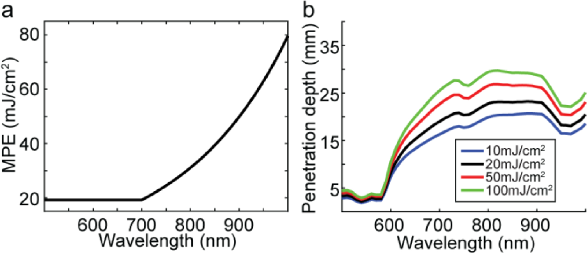
Simulation study. (a) MPE for skin in the range of 500–1000 nm based on ANSI standard, (b) maximum penetration depth at different fluence as a function of wavelength.

Here, we propose a computational method to increase the penetration depth of PAI. We used higher than ANSI limit laser energy in ex vivo brain imaging experiments, and used the obtained data as the training set for a deep learning algorithm. The trained deep learning kernel was then used to enhance the images generated in an in vivo experiment.

2 |. MATERIALS AND METHODS

2.1. PA Imaging System

A Q-switched Nd:Yag Opotek Phocus HE MOBILE laser (OPOTEK, LLC, USA) with the pulse width of 5 ns and the repetition rate of 10 Hz was used. The laser was tuned using an internal optical parametric oscillator (OPO). The laser energy was controlled with an internal attenuator. A single 10mm diameter plastic polymethyl methacrylate (PMMA) optical fiber (epef-10, Ever Heng Optical Co., Shenzhen, China) was coupled to the laser. For PA signal detection, an ATL L7–4 linear array (Philips, USA) ultrasound probe with 128-elements and 5MHz central frequency was used (element size: height, 7mm; width, 0.25mm), giving a penetration depth of ~4 cm in the brain tissue. Both the optical fiber and the probe position were held fixed with clamps. They were attached to an x-y stage for relative positioning. PA signal acquisition was performed using a 128-channel, high-frequency, programmable ultrasound system (Vantage 128, Verasonics Inc., USA). Both the data acquisition (DAQ) system and the laser flash lamp were triggered using a 10Hz square pulse train at 5V peak-peak generated by a function generator. The Q-switch was triggered by the Vantage 128. All the procedures were controlled through a Matlab graphical user interface. A schematic of the experimental setup is shown in Fig.2 (a).

FIGURE 2.

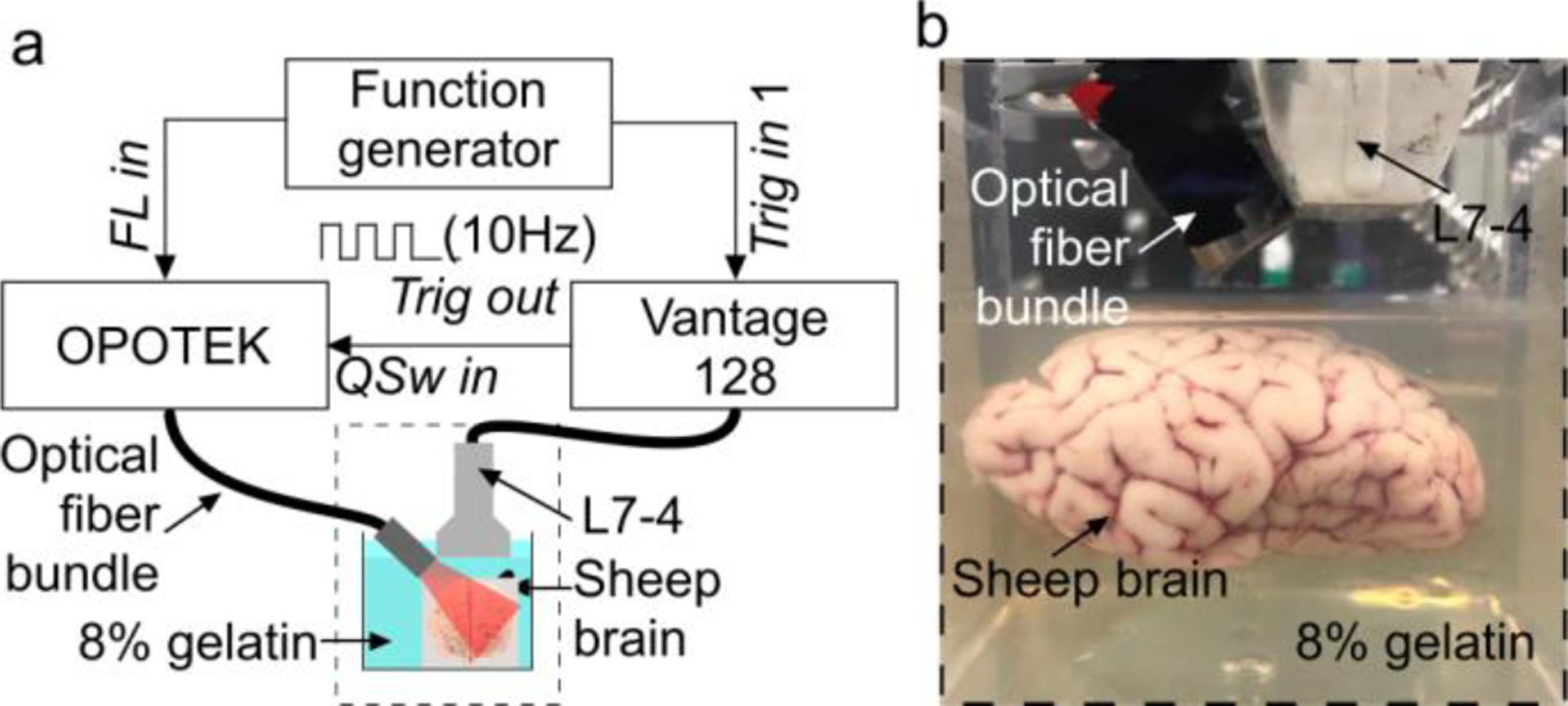
Ex vivo sheep brain imaging experimental setup. (a) Schematic of the experimental setup, (b) a photograph of a sheep brain phantom suspended in 8% gelatin. Trig: trigger, FL: flash lamp.

2.2. Ex vivo Brain Imaging Experiment

Freshly decapitated ~6-month old sheep heads were purchased from local slaughterhouse. A 6 cm diameter hole was drilled into the skull with a circular saw. The sheep brain was carefully brought out and preserved in the refrigerator. Later, the sheep brain was suspended in 8% porcine gelatin (Sigma Aldrich, St. Louis, MO, USA) approximately 5 mm below the top surface of the gelatin (see Fig.2 (b)). A transparent plastic container was used to hold the ex-vivo sheep brain in the gelatin and ultrasound gel was used as the coupling medium.

2.3. In vivo Brain Imaging Experiment

A 6-month old female sheep was acquired from the Michigan State University Farm (East Lansing, MI, USA) and sedated with acepromazine administered. Animal’s hair was removed from the dorsum of the skull using clippers and depilatory cream. Following the animal protocol approved by the Wayne State University Animal Care and Use Committee, two burr holes in the skull were made using a trepanation bit attached to a surgical electric drill, and then scalp was sutured. We waited 3 weeks for the animal to recover. The holes on the animal’s head were evaluated using CT scan (see Fig.3 (a)). While imaging, the PA probe was held fixed using a metal clamps connected to an optical table in order to avoid motion artifacts (see Fig.3 (b)).

FIGURE 3.

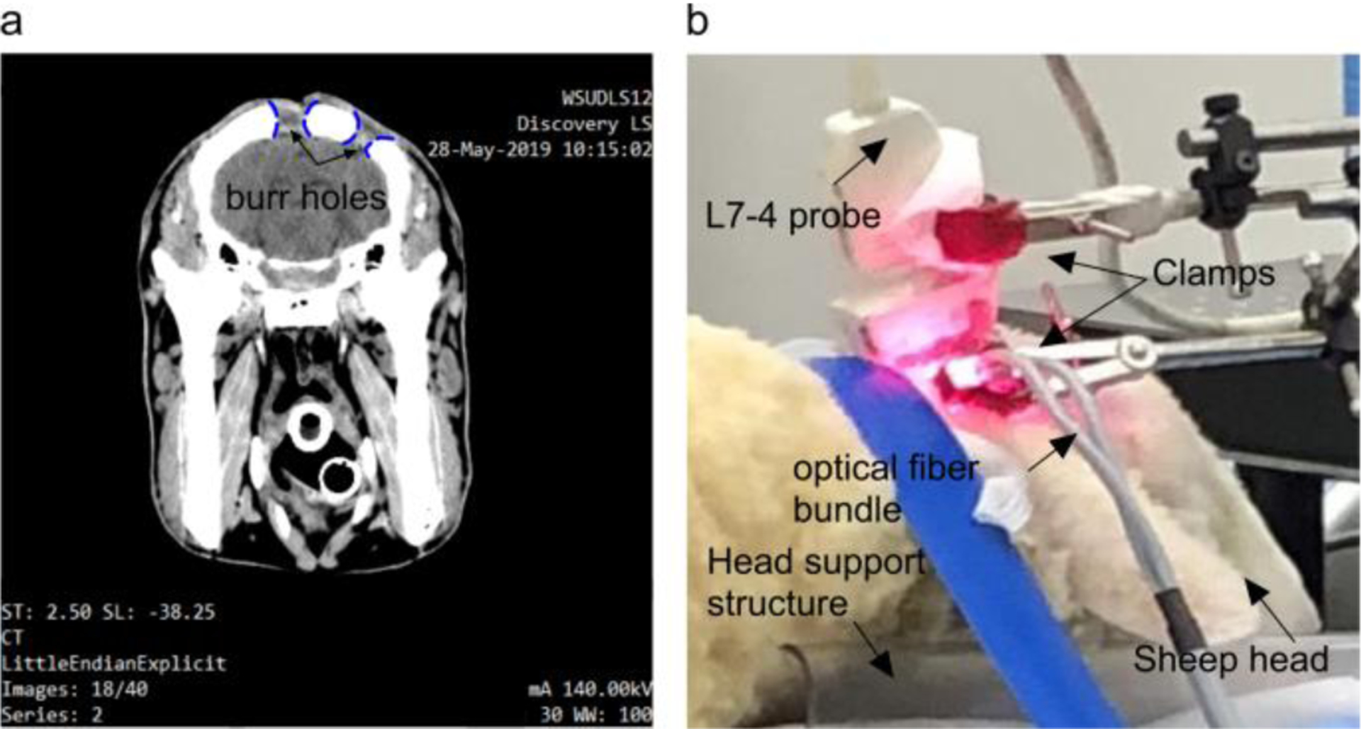
In vivo sheep brain imaging. (a) Sagittal view CT scan, and (b) in vivo experimental setup.

2.4. Implementation of Deep Learning Algorithm

U-Net is an efficient fully convolutional network (FCN) which has been used for many biomedical image analysis applications.

The main characteristic of U-Net that makes it suitable for the proposed application is its ability in combining the global spatial information and context information to make an image pattern prediction. Compared to many deep learning architectures that require complex design for the layers or a large amount of training datasets [8–10], U-Net can efficiently work with our limited datasets [11].

In this work, we have trained a U-Net with a perceptually sensitive loss function to learn how to enhance the low signal-to-noise ratio (SNR) structures in a PA image that were acquired with a low energy laser. The network design is shown in Fig.4. The neural network architecture consists of a contracting path: encoder (left) and an expansive path: decoder (right). The encoders consist of a repeated application of two 3×3 convolutional filters, each followed by a rectified linear unit (ReLU) and a 2×2 max-pooling operation with a stride of 2; for example, the first layer consists of 64 filters (with the size of 3×3) that are used to generate 64 feature maps and ReLU’s, while the final layer of the encoder consists of 512 filters to generate dense feature maps for the decoder. In order to mitigate overfitting, dropout was added between ReLU and max-pooling operations. For the decoder, the feature maps were expanded to the PA image in an inverse fashion. Each layer consists of a deconvolution of the feature map, concatenation with the feature map from the corresponding layer of encoder, and two 3×3 convolutional filters followed by the ReLU. The sigmoid layer was added to the final layer to predict an intensity value between 0 and 1.

FIGURE 4.

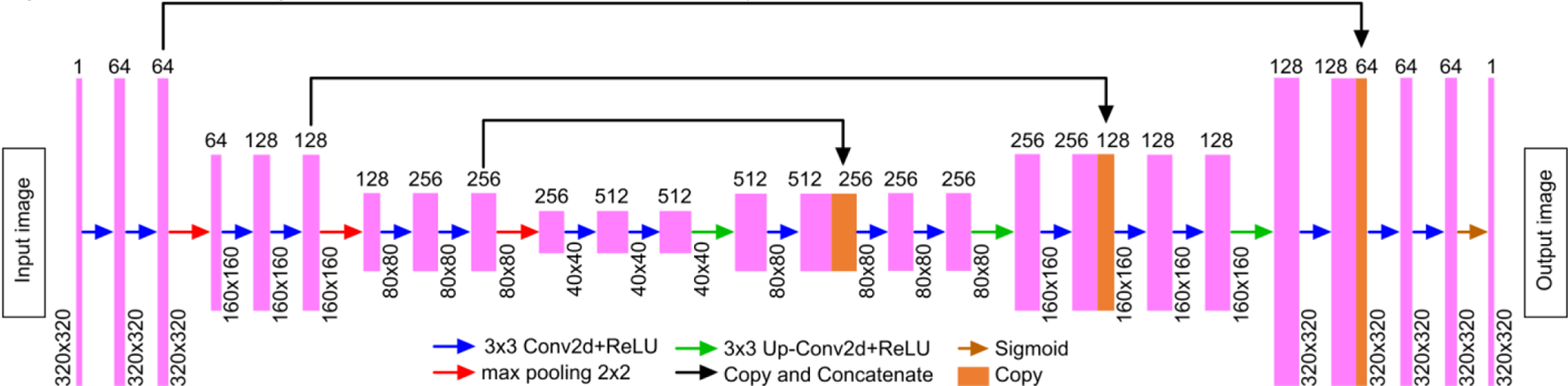
A schematic overview of the U-Net architecture used in this study.

Loss functions are vital in training deep learning models and affect the effectiveness and accuracy of the neural networks. We evaluated several loss functions including mean absolute error (MAE), mean squared error (MSE), structural similarity index (SSIM), multi-scale SSIM (MS-SSIM), and some recommended combinations in the literature including MS-SSIM + MSE and MS-SSIM + L1 [12]. Five quantitative measures including MAE, MSE, peak signal-to-noise ratio (PSNR), and SSIM were used for quantitative evaluation of the results [12].

2.5. Enhancement algorithm

We acquired B-scan images from the sheep brain, ex vivo, at both ~20 mJ and ~100 mJ (with illumination at 700 nm); measured by the laser built-in energy meter. Each imaging experiment was repeated 50 times to increase the SNR of the PA signals/ images. The B-scan images were captured from 100 different locations on the brain (~5 mm apart) along coronal and sagittal planes. The low energy images were used as the input data to the deep learning algorithm, and the high energy images used as label. We used 80% of the data for training and 20% for test. The trained kernel was then used to enhance the images generated in in vivo experiment.

3 |. RESULTS AND DISCUSSION

The U-Net was trained using the loss functions mentioned in Section 2.4. The quantitative results obtained with each of the loss functions for the entire dataset are listed in Table 1. The results indicate that SSIM+L1 and MS-SSIM+L1 are superior in all quantitative metrics. The training and validation loss of these loss functions in 50 epochs shown in Fig. 5(a) and (b), indicating that the training is converged. The hyperparameters (i.e., training batch size and learning rate) are sufficiently tuned to achieve a minimal overfitting, which is evident by the small gap between training and validation losses. The results of the trained deep learning kernel on an arbitrary low-energy-laser generated ex vivo image with the two optimum loss functions are given in Fig.6. The observations are as follows: the PA images acquired at 100 mJ visualized lateral ventricles, hippocampus as well as deeper vasculatures (see the main structural features in Fig. 6(a) and (b)), whereas at 20 mJ, the visible structures are limited to superficial vasculatures only (see Fig. 6(c) versus Fig. 6(d)); the visibility of the structures in the deep-learning-enhanced PA image has increased (compare Fig. 6e(i), and e(ii)). We plotted a depth profile of the PA image generated by a low energy laser and compared that with the depth profile of the PA image generated by a high energy laser, and also with the deep learning enhanced images (see Fig. 6(f)). Further, we calculated the peak-to-background ratio (PBR) for all A-lines in each of the PA images mentioned above and averaged. The penetration depth in the image was also calculated based on 5% of the A-line maximum fall off. The deep learning kernel increased the PBR by 5.53 dB, and the penetration depth by 15.6%, compared to those of the low energy generated PA images.

TABLE 1.

Quantitative analysis. MAE: mean absolute error, MSE: mean squared error, PSNR: peak signal-to-noise ratio, SSIM: structural similarity index, MS-SSIM: multi-scale SSIM.

Type	MAE	MSE	SSIM	MS-SSIM	SSIM+L1	MS-SSIM+L1
MAE	0.01935	0.0832	0.022995	0.4294	0.014	0.015
MSE	0.0011	0.01	0.0015	0.1856	0.0007799	0.0008
PSNR	29.58	19.258	28.19	7.31	31.079	31.01
SSIM	0.9184	0.0817	0.90129	0.2979	0.9354	0.934

FIGURE 5.

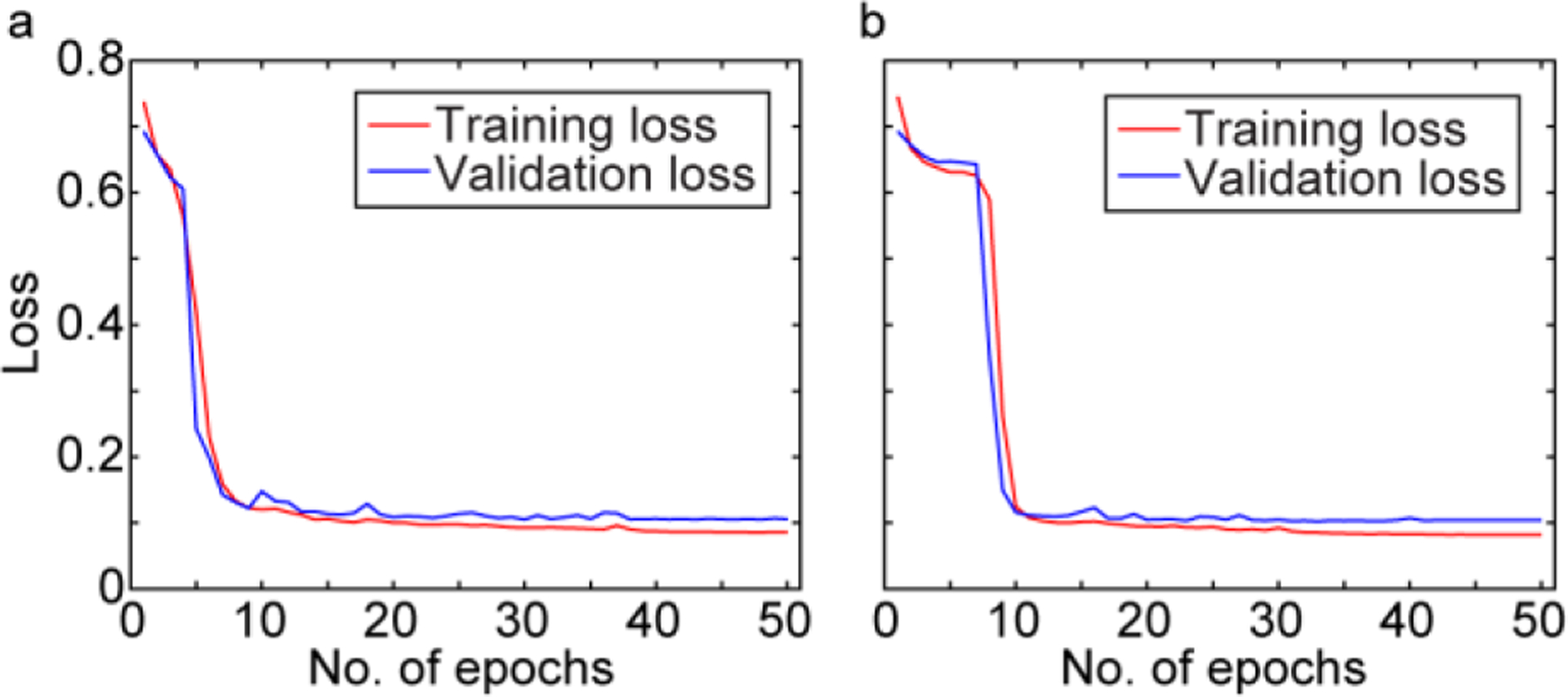
Training and validation loss of (a) MLSSIM+L1 and (b) SSIM+L1, as a function of number of epochs.

FIGURE 6.

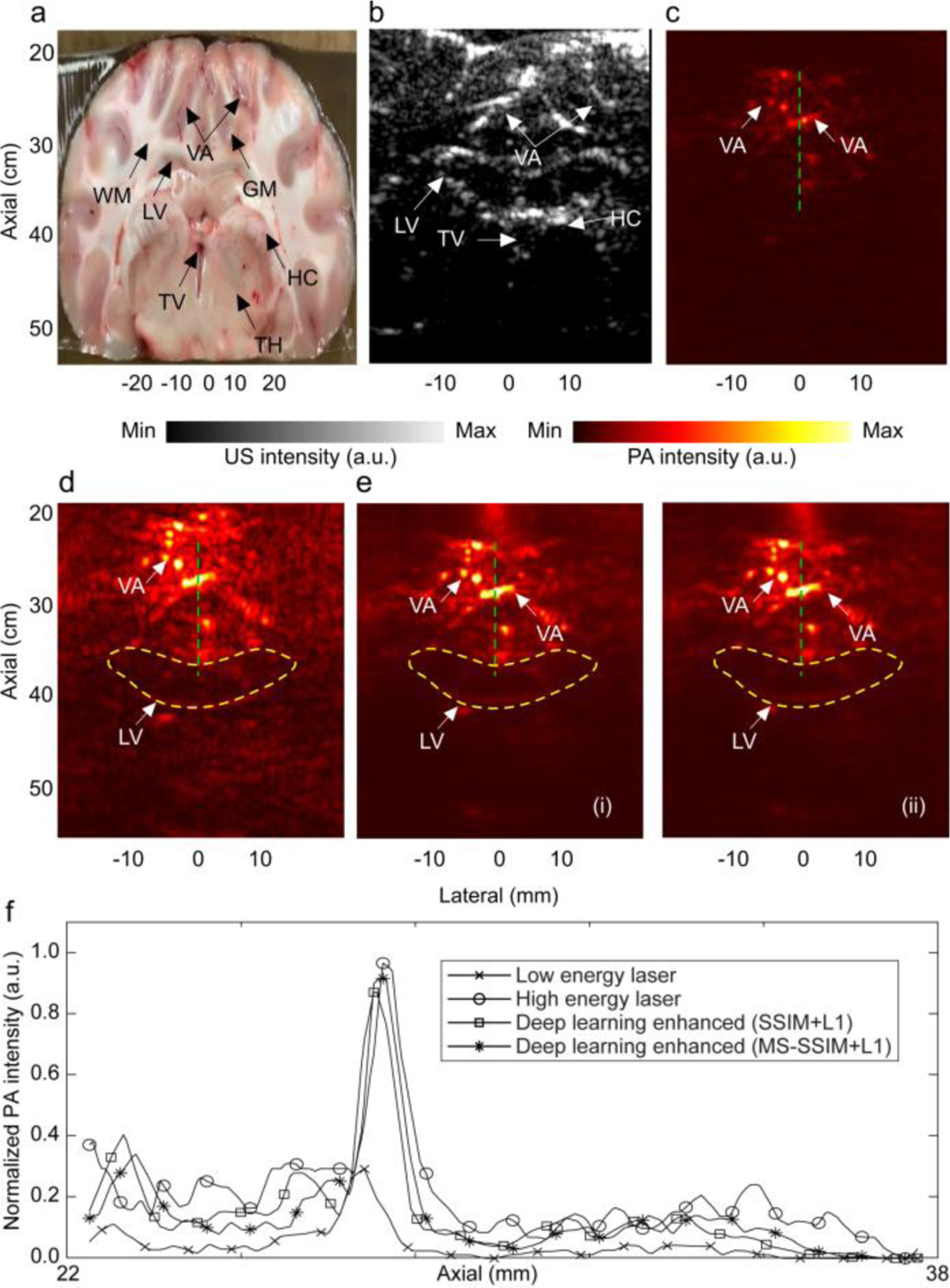
Evaluation of the performance of the trained U-Net kernel on PA images of ex vivo brain. (a) Cross-sectional image of the sheep brain along the coronal plane, (b) US image, (c) PA image generated with low laser energy (~20mJ), (d) PA image with high laser energy (~100mJ), (e) deep learning enhanced PA image in (c), with (i) SSIM+L1 loss function, and (ii) MS-SSIM+L1loss function, (f) sample depth profiles of PA images in (c), (d), and (e) along the green dashed line as indicated. Yellow contours indicate some of the structures which were not present in (c). WM: white matter, LV: lateral ventricle, GM: grey matter, HC: hippocampus, TV: third ventricle, TH: thalamus, VA: vasculature.

We then used the deep learning kernel trained with SSIM+L1 and MS-SSIM+L1 loss functions to enhance the PA images obtained from the in vivo experiment. The results are shown in Fig. 7. After the enhancement, outline of the deeper structures such as lateral ventricle, third ventricle became more prominent. Several vasculatures within the grey matter were also distinguishable which were not even visible in the original reconstructed image. The PBR in the enhanced image was improved by 4.19 dB and the penetration depth, by 5.88%.

FIGURE 7.

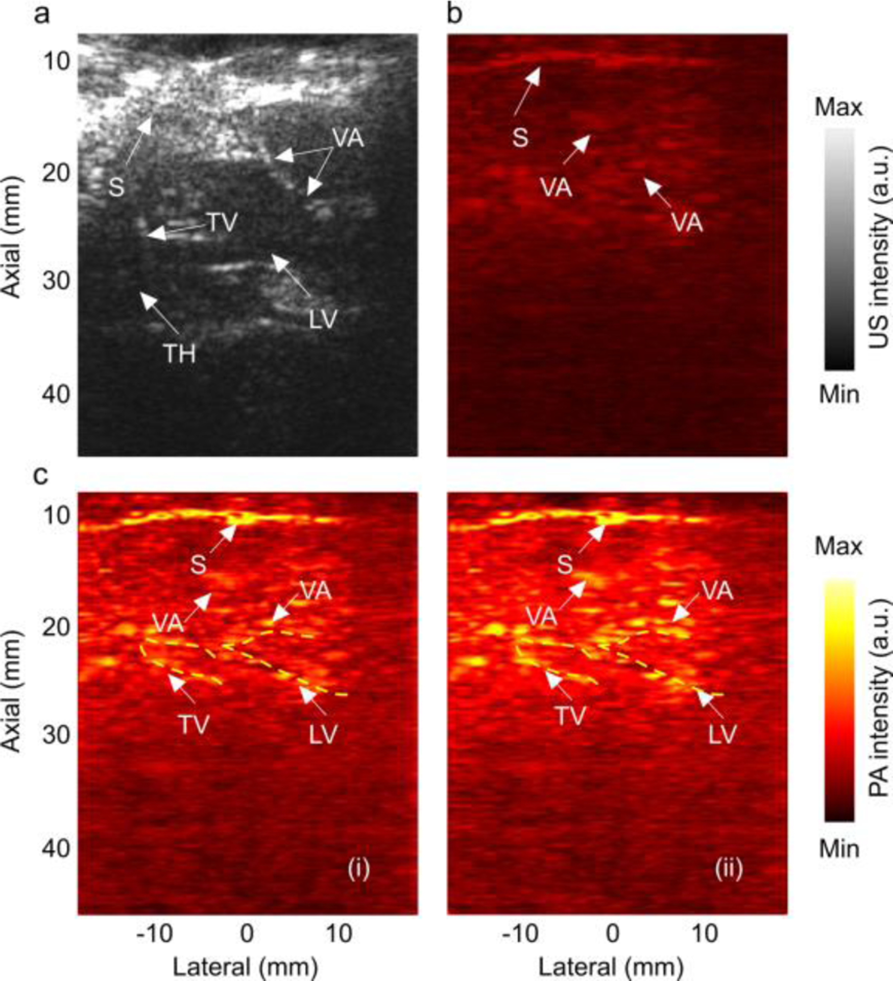
Evaluation of the performance of the trained U-Net kernel on in-vivo sheep brain images. (a) US image along sagittal plane, (b) PA image generated with low energy laser, (c) deep learning enhanced PA image in (b), with (i) SSIM+L1 loss function, and (ii) MS-SSIM+L1loss function. S: skin. LV: lateral ventricle, TV: third ventricle, TH: thalamus, VA: vasculature. Yellow contours indicate some of the structures which were not present in (b).

4 |. CONCLUSION

In this work, we proposed an effective deep learning network trained with perceptually-sensitive loss functions to enhance PA images of the brain in an in vivo experiment generated by a low energy laser light. Using the deep learning kernel, we increased the SNR of the deep structures surrounding lateral and third ventricles that were not present in the PA image generated by a low energy laser. We believe this computational kernel facilitates future efforts toward clinical translation of PAI in brain imaging, especially neonatal brain imaging, where transfontanelle imaging is possible.

REFERENCES

- [1].Nasiriavanaki M, Xia J, Wan H, Bauer AQ, Culver JP, Wang LV, Proceedings of the National Academy of Sciences 2014, 111, 21–26. [DOI] [PMC free article] [PubMed] [Google Scholar]
- [2].Sona A, International norms and EC directives on laser safety in medicine and surgery, Laser Florence 2003: A Window on the Laser Medicine World, International Society for Optics and Photonics, 2004, pp. 60–64. [Google Scholar]
- [3].ANSI, 2014.
- [4].Hecht J, 2008.
- [5].Chao CP, Zaleski CG, Patton AC, Radiographics 2006, 26 Suppl 1, S159–172. [DOI] [PubMed] [Google Scholar]
- [6].Jacques SL, Physics in Medicine & Biology 2013, 58, R37. [DOI] [PubMed] [Google Scholar]
- [7].Fang Q, Boas DA, Optics express 2009, 17, 20178–20190. [DOI] [PMC free article] [PubMed] [Google Scholar]
- [8].Oktay O, Schlemper J, Folgoc LL, Lee M, Heinrich M, Misawa K, Mori K, McDonagh S, Hammerla NY, Kainz B, arXiv preprint arXiv:1804.03999 2018. [Google Scholar]
- [9].Azad R, Asadi-Aghbolaghi M, Fathy M, Escalera S, Bi-Directional ConvLSTM U-Net with Densley Connected Convolutions, Proceedings of the IEEE International Conference on Computer Vision Workshops, 2019, pp. 0–0. [Google Scholar]
- [10].Hariri A, Alipour K, Mantri Y, Schulze JP, Jokerst JV, Biomedical Optics Express 2020, 11, 3360–3373. [DOI] [PMC free article] [PubMed] [Google Scholar]
- [11].Ronneberger O, Fischer P, Brox T, U-net: Convolutional networks for biomedical image segmentation, International Conference on Medical image computing and computer-assisted intervention, Springer, 2015, pp. 234–241. [Google Scholar]
- [12].Qiu B, Huang Z, Liu X, Meng X, You Y, Liu G, Yang K, Maier A, Ren Q, Lu Y, Biomedical Optics Express 2020, 11, 817–830. [DOI] [PMC free article] [PubMed] [Google Scholar]