

Abstract
Background and objective
The availability of labeled data is crucial for training deep neural networks. However, in some cases, the available data is limited or unlabeled, which poses a significant obstacle in developing accurate models. Various approaches exist to address this issue, such as Image Augmentation, Transfer Learning, and GANs. However, these approaches often require a significant amount of training data or may not generate desired results. In this article, we present a novel method for generating synthetic images from very limited data using the ACGAN.
Methods
We conducted experiments on a real dataset consisting of 198 ultrasound images of calcified and cystic thyroid gland nodules. We explored and improved different architectures and techniques in the Axillary Classifier Generative Adversarial Network (ACGAN) to generate high-quality synthetic images. To evaluate the generated images, we used the Fréchet Inception Distance (FID) test and human observation. Additionally, we developed an image blending method to generate larger images that simulate the output of an ultrasound device. To validate the accuracy of the merged images, a specialist doctor reviewed the generated data.
Results
The modified ACGAN architecture successfully generated new synthetic images from limited data. The output images were assessed based on the image progress ratio with the FID test and human observation. Moreover, the Image blending method was successful in producing larger output images that mimic the nature of the ultrasound device output images. The final merged images were validated by a specialist doctor who confirmed their accuracy.
Conclusions
Our method has significant implications for medical imaging, as it enables the generation of synthetic labeled data for training deep learning models, leading to better diagnostic accuracy and improved patient outcomes. This study provides a proof-of-concept for generating synthetic medical images from limited labeled data and can inspire future research in this area.
Keywords: Limited data, Synthetic images, Medical imaging, ACGAN, Thyroid gland, Image blending
Introduction
Scientists and technologists have heavily invested in hardware and software for various applications [1]. However, creating a deep neural network for medical image processing and classifying multiple datasets, including medical images is challenging due to ethical concerns about sharing patient photos. It is also difficult to find a specialist to annotate ultrasonography, PET, CT, and MRI imaging data [2]. Additionally, inadequate training data or the absence of labeled data results in inadequate training data, preventing the network from learning the given data, and archiving the intended output.
Production of images using (ACGAN)
In recent years, GAN networks [3] have been utilized in several medical applications [4, 5] to create accurate data categorization [6]. Some publications aim to identify the optimal image-generating technique or enhance the outcome by combining multiple methods. In this article, we employ a conditional adversarial deep network called ACGAN to produce new images while facing data restrictions. We evaluate various architectures for building a network that can generate new images from a limited dataset, and then seek to create a larger output image dataset. Augustus Odena demonstrated that using an auxiliary class improves image generation, especially when the network has a limited number of input data [7]. Therefore, we chose this network to investigate new changes for limited data, using input data to produce images ranging from 64 × 64 to 256 × 256 pixels.
The lack of data in any field, especially medicine, as discussed by [8]. Despite the scarcity of input data, the authors challenge the network to generate images using Transfer Learning. Similarly, we challenge the ACGAN network by using only 198 input images of the thyroid gland prepared by Mashhad University of Medical Sciences (see Fig. 1) to train the network and generate large images resembling original ultrasonography images by merging small generated shots into another main image with a simple ultrasonographic texture. Recent studies such as [9, 10], and [11] have used the picture-blending technique exclusively in the medical research sector, demonstrating its efficacy. However, they all use a costly, time-consuming deep convolution network training approach. We employ fundamental image processing methods, including identically formatted photographs in the final material.
Fig. 1.

Sample of data in the dataset. The image on the right depicts a portion of the thyroid gland with calcification nodules, and the image on the left shows a thyroid gland with a cystic nodule
Sampling input images
The paper by [12] uses the Patching method to distinguish the input ROI image from the original photos. The images are sampled, and fed to a network that is trained on them. A new conditional function is then introduced to the ACGAN network to obtain a positive result. Additionally, the Cropping technique is utilized (as shown in Fig. 2) to leverage the created margins and enhance blending with the background.
Fig. 2.

ROI of ultrasonographic thyroid nodule
In this study, we clip the area of interest to be added to the ultrasound image. However, to accomplish this, it is essential to consider three issues that make picture composition challenging:
Understanding the nature and components of an image to associate it with the object or second image.
In some cases, creating an element other than the objects in the image is necessary to fit well with the angles and dimensions of the backdrop image.
Selecting the appropriate approach to add the images to the primary or, in some circumstances, background image to generate an acceptable output is vital.
Generating large images
Spatial Transformer Generative Adversarial Networks (ST-GAN) for Image Compositing [10], has explored the formation of large images by combining two images using a GAN network. The network detects objects in the images and generates new ones that add the second image to the first image, depending on the input image. Authors in [13] paper used image feature extraction approaches, such as locating the edge and deleting values from other pixels that do not match the two images’ values, to optimize transformation and image blending for 3D liver ultrasound series stitching. Similarly, [11] employed Homomorphic Alpha Blending of Long Bone Digital Radiography Images to combine images and create an anatomy image. In [14] two fluoroscopy images were merged using edge detection and similarity recognition.
In all the provided publications, a deep neural network is used to merge two radiological and ultrasound images. However, the ultrasound image blending approach does not pose a challenge because it simply adds a newly generated piece of the image to a larger image with dimensions of 1024 by 1024 pixels, which is the size of an ultrasound image of healthy tissue surrounding the larynx.
Methods
Generating new data
In order to increase the size of our dataset, we used Keras’ Image Augmentation technique and Image Generation function to augment the photos. This resulted in an increase in the dataset from 198 to 510 images. We took care to ensure that these small changes did not interfere with our goal of training a network with limitations.
Training process
The training process consists of two components. First, we randomly arranged two thyroid gland pictures with cysts and calcifications classes. Second, we stored data of the same kind in a CSV file that will be subsequently used as network input. By combining these two components, we were able to effectively train our network.
Execution environment
Image processing calculations require a powerful system. Therefore, we utilized the Google Colab Pro platform with 12 gigabytes of RAM and an Nvidia V100 GPU processor to train and analyze the input data. We took care to ensure that we followed all necessary copyright rules and regulations during the entire process. We also made sure to properly cite any sources that we used in our research.
Network architecture
To produce the final images using our proposed architecture on the ACGAN network and the functional programming method in Keras [15], various values are added together in this type of network after undergoing multiple operations. We must be cautious with excessive training to avoid becoming trapped in GAN convergence issues [16].
Consequently, for this project, we will use the below implementation strategy, as we must apply numerous network layers and parameters. The following articles were used to achieve our desired outcomes [17–21]. Based on this, our proposed architecture corresponds to Fig. 3.
Fig. 3.

Proposed network architecture
Results evaluation
Due to the absence of a specific method for determining the quality of an image, the evaluation of produced images is typically conducted by human observers. However, in recent years, new techniques such as the FID (Fréchet Inception Distance) have been developed for calculating image quality [22]. This technique is named after the mathematician René Maurice Fréchet, who calculated curvature and probability distribution. One of the conventional ways to illustrate the Fréchet Distance is by using the Dog-walker problem, in which a dog and a human move forward at a desired speed only and they cannot return. To calculate the distance between the created lines, the minimum length of the collar from the start of the path to its end must be known. This distance can also be calculated using the probability distribution and Eq. 1 provided below:
| 1 |
In the above equation, the represents the median rate and indicates the mean cost between humans and dogs. Additionally, which represents indicated by sigma, is the amount of deviation from the standard or distribution of this distance. It should be noted that a lower FID value indicates a closer distribution sign. Using this method and the trained INCEPTIONv.3 model, which was trained with ImageNet images, the degree of proximity and similarity between the images can be estimated.
Coding
Since our output requires two values- the probability of the class type and the likelihood of the picture type- we used the Functional API technique in Keras.
After processing the pictures and labels, the main function reads the functions of the Discriminator and Generator networks. The pixel data generation function inputs the data into the Generator. The real image input function is then called, and the main function inspects 50 samples at a time through a multi-thousandth loop rejection process. Newly generated data are examined, and later the accuracy and loss diagram are produced. The freshly developed photos are selected for display in the output, and an h5 model sample is formed for further utilization.
In a separate function, the FID measurement test compares each phase's photographs to the original input images. The high-scoring photos are added to the plain ultrasound images to create a larger final image. Our network design is based on the primary article Auxiliary Classifier GAN. We assessed network configurations based on [17–21]. It can be difficult to select the appropriate architecture and hyperparameters to generate new and vast data from limited data. Our proposed network architecture has two main functions, which are described below.
The Discriminator, has two inputs—the actual image and the output—that indicate the likelihood of the real-world image corresponding to the predefined classes. This network can process input images of two classes ranging from 28 × 28 × 1 to 256 × 256 × 1 as input images. This network uses Gaussian Weight initialization with a standard deviation of 0.02, Batch normalization, a LeakyReLU activation function with an alpha value of 0.2, and a Dropout value of 0.5. Gaussian noise is added in every six convolution layers, and one in between layers, a 2 × 2 downsampling takes place. The network has two output layers, the first using the Sigmoid activation function to differentiate between real and fake data, and the second containing multiple nodes to determine the probability of two classes given an image as input, using the Softmax activation function. The network uses binary cross-entropy cost functions for the first output, categorical cross-entropy loss for the second output, data accuracy criteria, and the Adam function with a learning rate of 0.002 and a Momentum value of 0.5 to update the network.
The Generator, which uses a random value from the noise space (110) and an embedded function of (50) to combine classes in our selected dimensions, is utilized to improve the output by labeling names. An additional feature map layer enhances the output from a fully connected layer with a linear activation function. The Noise space needs a layer with enough activators to generate 385 feature maps. At each upsampling step, the transpose convolution layer doubles the reduced image. Each step produces n x n images, which are optimized using Batch normalization and the ReLU activator function before being sent to the next layer. As the hyperbolic tangent activation function is used, the final output value of the Generator function for each image ranges from − 1 to 1.
After training the network and obtaining the trained model, we create images with the option to choose the data class and as many as needed by providing a noise space and presenting it to the model.
The sci-kit-image library and Image Pillow library can blur the edges of photos to make them look more realistic. The background of healthy thyroid tissue is obscured. This method enables us to insert the second photo at a specific pixel coordinate location.
Results
Results assessment
Data creation may fail due to excessive network hyperparameter configurations, leading to diverse outcomes. The resulting output is subpar, with a significant error rate. However, a network with the following specifications has the potential to generate satisfactory images:
If discriminator loss is approximately 50%.
If the generator’s loss ranges from 50 to 200%.
If the data accuracy hovers around 80%.
If both generator and discriminator loss remain stable.
If the generator produces its best images when training stabilizes.
It is essential to avoid further training once training stability is reached.
To evaluate each method’s effectiveness, we initially tested the mentioned elements for creating 28 × 28 pictures. The network’s architectural parameters were sequentially analyzed and combined to determine the effective combinations.
28 × 28 size data output
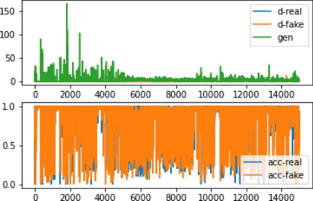
After training the network for three hours using the GPU system provided by the Google Colab website for three hours, and repeating the learning process up to 100,000 times to learn input photographs of 28 × 28 pixels, the results remained unclear. However, after 35,000 training repetitions, as depicted in Fig. 4, the network has reached a point where the accuracy ratio between real and artificial data could be distinguished. Table 1 demonstrates that the loss amount in the synthetic data is certain compared to the original data. Furthermore, Fig. 5 illustrates the high accuracy value when comparing the original image with the produced image. To ensure a fair comparison, the original photo was scaled to 28 × 28 pixels, and Fig. 6 shows that the produced classes contain many details but appear highly pixelated.
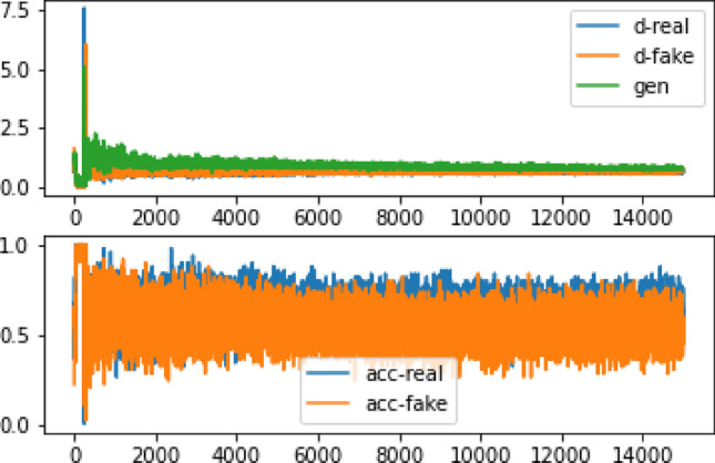
Fig. 4.

The accuracy and inaccuracy of the 28 × 28 image data after 100,000 repetitions. d-real represents the error in detecting the realness of the information by the discriminator, while d-fake shows the error in detecting the falsity of a statement. Moreover, gen indicates the accuracy of detecting real data, and acc-real: reflects the accuracy of detecting simulated data
Table 1.
Accuracy and error percentage of 28 × 28 images
| Accuracy | Loss% | |
|---|---|---|
| Discriminator fake data | 76% | 70 |
| Discriminator real data | 74% | 68 |
| Generator loss | – | 77 |
Fig. 5.
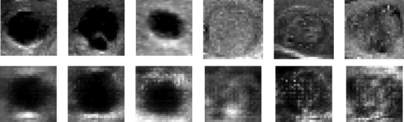
Comparison of the 28 × 28 production images with real photos. The top row images are the main images, and the bottom ones are production images of 28 × 28 pixels
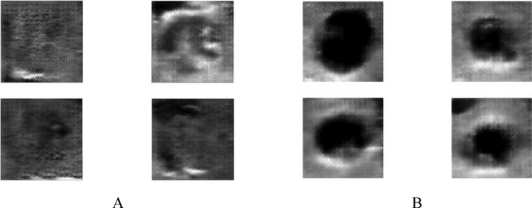
Fig. 6.

Quadruple view of produced class images 28 × 28 in two classes A calcification mass B cystic gland
32 × 32 size data output
After training the network for 26 min and repeating the learning process up to 15,000 times to understand 32 × 32 input images, the output shows improved clarity compared to 28 × 28 images. This finding aligns with the study by [7], which suggests that increasing the size of the input data can lead to better output images. By comparing Fig. 7 with Fig. 6, it becomes apparent that image size positively influences recognition and output quality.
Fig. 7.

Quadruple view of 32 × 32 created class pictures in two separate classes A calcification mass B cystic gland and
Figure 8 shows that after 15,000 training repetitions, the network achieves an accuracy of 70–80% and a loss of 60% Table 2. In addition, when comparing the FID test results of 28 × 28 and 32 × 32 pixel pictures, there were only marginal differences observed in the images of cystic nodes and calcification Table 3. Therefore, upon analyzing the impact with the original image, it is evident that the results are improved, albeit still displaying some pixelation Fig. 9.
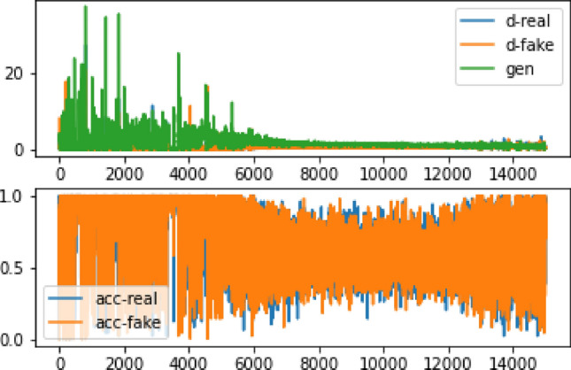
Fig. 8.
The accuracy and inaccuracy of the 32 × 32 image data after 15,000 repetitions. d-real represents the error in detecting the realness of the information by the discriminator, while d-fake shows the error in detecting the falsity of a statement. Moreover, gen indicates the accuracy of detecting real data, and acc-real: reflects the accuracy of detecting simulated data
Table 2.
Accuracy and loss percentage of 32 × 32 images
| Accuracy | Loss% | |
|---|---|---|
| Discriminator fake data | 76% | 67 |
| Discriminator real data | 80% | 65 |
| Generator loss | – | 80 |
Table 3.
Comparing the similarity of 28 × 28 and 32 × 32 images
| FID | Same | Different |
|---|---|---|
| Cystic | − 0.00 | 70 ± 150 |
| Calcification | − 0.00 | 80 ± 100 |
Fig. 9.

Comparison of the 32 × 32 production images with real photos. The top row images are the main images, and the bottom ones are production images of 32 × 32 pixels
64 × 64 size data output
To construct 64 × 64 photos, the network underwent training for a maximum of 15,000 iterations Fig. 10. After 48 min and 12,400 iterations, we obtained the result Fig. 11 with accurate error values, thus affirming the learning capabilities of the network Table 4. However, it is evident from the image that the generated photos lack clarity and quality when compared to authentic images of the same size Fig. 12. This discrepancy is also noticeable when contrasting these generated photographs with the smaller ones Table 5.
Fig. 10.

The accuracy and inaccuracy of the 64 × 64 image data after 15,000 repetitions. d-real represents the error in detecting the realness of the information by the discriminator, while d-fake shows the error in detecting the falsity of a statement. Moreover, gen indicates the accuracy of detecting real data, and acc-real: reflects the accuracy of detecting simulated data
Fig. 11.
The quadruple perspective of 64 × 64 generated class photographs for two distinct courses. A calcification mass vs. B cystic gland
Table 4.
Accuracy and a loss percentage of 64 × 64 images
| Accuracy | Loss% | |
|---|---|---|
| Discriminator fake data | 77% | 66 |
| Discriminator real data | 79% | 64 |
| Generator loss | – | 86 |
Fig. 12.

Comparison of the 64 × 64 production images with real photos. The top row images are the main images, and the bottom ones are production images of 64 × 64 pixels
Table 5.
Comparing the similarity of 64 × 64 and 32 × 32 images
| FID | Same | Different |
|---|---|---|
| Cystic | − 0.00 | 130 ± 140 |
| Calcification | − 0.00 | 120 ± 150 |
128 × 128 size data output
After 1 h and 30 min of training with 12,100 epochs, we obtained the output shown in Fig. 13, along with the accuracy and error diagram depicted in Fig. 14. The network achieved an accuracy of 80%, and a loss rate of 55% after 13,000 iterations, as shown in Table 6. These figures indicate successful convergence and optimal outcome generation. By comparing the 64 × 64 pictures to the 128 × 128 images presented in Table 7, it is evident that the current photos exhibit a significant greater improvement, and disparity compared to the smaller image shown in Fig. 11, as opposed to Fig. 13. Further comparison of our findings with the original data is illustrated in Fig. 15, which clearly demonstrates this improvement.
Fig. 13.

The quadruple perspective of 128 × 128 produced class images for two separate classes. B calcification mass as opposed to A cystic gland
Fig. 14.
The accuracy and inaccuracy of the 128 × 128 image data after 15,000 repetitions. d-real represents the error in detecting the realness of the information by the discriminator, while d-fake shows the error in detecting the falsity of a statement. Moreover, gen indicates the accuracy of detecting real data, and acc-real: reflects the accuracy of detecting simulated data
Table 6.
Accuracy and loss percentage of 128 × 128 images
| Accuracy | Loss% | |
|---|---|---|
| Discriminator fake data | 87% | 57 |
| Discriminator real data | 89% | 55 |
| Generator loss | – | 80 |
Table 7.
Comparing the similarity of 128 × 128 and 64 × 64 images
| FID | Same | Different |
|---|---|---|
| Cystic | − 0.00 | 150 ± 197 |
| Calcification | − 0.00 | 180 ± 200 |
Fig. 15.

Comparison of the 128 × 128 production images with real photos. The top row images are the main images, and the bottom ones are production images of 128 × 128 pixels
256 × 256 size data output
The output photos are improved due to the larger size of the input images. Following 15,000 iterations, the output graph exhibits a substantial rate of change and non-convergence at one point. However, through a step-by-step evaluation of the production model, it achieves results that closely approximate reality in steps 13,800 Figs. 16 and 17. Table 8 shows a 45% loss and 90% accuracy. Figure 18 illustrates the alignment between the findings and the real images. Based on Table 9, the ratio of picture modifications from 128 × 128 to 256 × 256 remains relatively consistent. Furthermore, Table 10 reveals that while some generated images exhibit minor differences from the original images, others display significant disparities.
Fig. 16.

The 256 × 256 quadruple perspective generated class pictures for two distinct classes compared to A calcification mass B cystic gland
Fig. 17.
The accuracy and inaccuracy of the 256 × 256 image data after 15,000 repetitions. d-real represents the error in detecting the realness of the information by the discriminator, while d-fake shows the error in detecting the falsity of a statement. Moreover, gen indicates the accuracy of detecting real data, and acc-real: reflects the accuracy of detecting simulated data
Table 8.
Accuracy and a loss percentage of 256 × 256 images
| FID | Same | Different |
|---|---|---|
| Cystic | − 0.00 | 110 ± 240 |
| Calcification | − 0.00 | 22 ± 166 |
Fig. 18.

Comparison of the 256 × 256 production images with real photos. The top row images are the main images, and the bottom ones are production images of 256 × 256 pixels
Table 9.
Comparing the similarity of 256 × 256 and 128 × 128 images
| Accuracy | Loss% | |
|---|---|---|
| Discriminator fake data | 92% | 45 |
| Discriminator real data | 93% | 46 |
| Generator loss | – | 82 |
Table 10.
Comparing the similarity of 256 × 256 and real images
| FID | Same | Different |
|---|---|---|
| Cystic | − 0.00 | 20 ± 50 |
| Calcification | − 0.00 | 15± 25 |
Blending two images
By employing the Image Composition technique, we utilized the Pillow library to construct a large-scale ultrasound image. In order to enhance realism, we seamlessly combined the background and production image textures. Circular blurring at the corners of the image is depicted in Fig. 19. This successful process was implemented using the Scikit-image package, as evident in the output images.
Fig. 19.
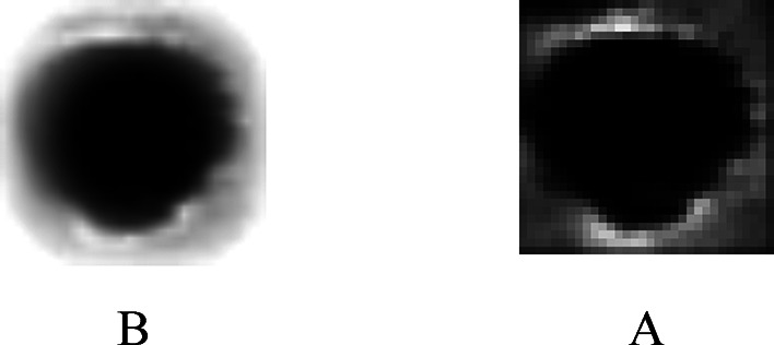
The output picture A transformation into the final image. B
Three components are necessary for achieving realistic visuals:
When generating fake pictures from small images, it is essential to reduce their dimensions to improve clarity, as they tend to appear opaque even when scaled to larger proportions.
The choice of backdrops significantly impacts the quality of the photos. It is crucial to use backgrounds that are different from the ones used for both classes, as depicted in Figs. 20 and 21.
Even after blurring the boundaries, certain generated images may not seamlessly integrate with the background. Therefore, color and light editing is required to enhance authenticity and ensure a natural placement effect.
Fig. 20.

Embedded image of cystic thyroid nodule
Fig. 21.

Embedded image of calcification thyroid mass
Evaluation of final images
Three specialist medics assessed the completed shots for their structure, resemblance, and defects. This examination included 100 production shots divided into two groups. According to expert physicians, by analyzing the photographs and employing the ACR-TIRADS standard, it becomes possible to differentiate between benign and malignant nodules in the images, and the fact that these images are not real is not readily apparent. The TIRADS standard was used to classify the existing images, although some proved too complex for recognition. Medically, a doctor who performs ultrasonography by manipulating the ultrasound probe provides a more accurate diagnostic. Based on the doctor's assessments, over 90% of the images could be categorized, and those that were challenging to diagnose did not pose any issues regarding the nature and quality of the image (see Table 11).
Table 11.
The outcomes of the physician's examination
| Expert physician | Real image% | Artificial images% | TRADS class detection% |
|---|---|---|---|
| Physician 1 | 79 | 70 | 61 |
| Physician 2 | 73 | 68 | 60 |
| Physician 3 | 72 | 64 | 58 |
Discussion
After the training phase, the image classification system demonstrated accurate recognition of 100 images from each category Fig. 22. Despite the limitations imposed by the available data, it was observed that larger image sizes contributed to reduced convergence time and facilitated the achievement of optimal results. The size of the region of interest (ROI) images ranged from 27 × 27 to 290 × 290 pixels. Following the preprocessing step of equalizing the input pictures in the network, some of the smaller output images exhibited a matte appearance. These images were found to be more suitable for applications with small production sizes, such as 23 × 32 pixels. Consequently, the network was trained with images of various sizes, allowing each iteration to generate distinct visuals characterized by clarity, fading, or windowed effects, depending on the input type and size. Due to the limitations of the dataset, there existed a risk of photo duplication or network overfitting. However, given the diversity of the images and the multiple alternatives available during each step of image synthesis, even identical shots exhibited subtle variations. Taking into account factors such as background, picture size, color, and lighting, the final photos appeared remarkably realistic. Ultimately, these lifelike photographs facilitated the classification and identification tasks performed by domain specialists.
Fig. 22.

A One hundred outputs of both classes A: the cystic and B calcification
We adopted a comprehensive approach to investigating the production of realistic images, employing pictures of calcified masses and cyst nodules that varied in size from 28 by 28 to 256 by 256 pixels. This article addresses the assumptions arising from real-world scenarios where we encounter a limited dataset. Therefore, the dataset utilized in our study consisted of 198 photos, which we augmented to 510 for improved network training. Consequently, we examined image generation and developed the final architecture for producing images using the ACGAN network structure. To accomplish this, we followed the settings and parameters recommended in the papers, allowing us to construct a network capable of generating new photos even when faced with data constraints.
Our ultimate goal was to generate ultrasound images that accurately depicted the details of cystic and calcification nodules. This was achieved by integrating production photos into the background image, leveraging the capabilities of Scikit-image and Pillow libraries. These libraries are robust image-processing packages, and the resulting images closely resembled the original complete ultrasound images.
Conclusions
This study analyzes the potential of adversarial generating networks and directly addresses the issue of insufficient data by generating images from limited datasets. Despite these limitations, the combination of the generated pictures into the ultrasound backdrop image results in 1024 × 1024 images that exhibit a resolution comparable to the original images.
In this research, we examined each of the additional network architecture parameters of ACGAN individually and in more than ten combinations. However, most of the results did not align with our predictions, and we were unable to achieve favorable outcomes. We discovered that, with limited data, the network noise layer, Label smoothing, and Noisy labels play a crucial role in generating new images. Additionally, the Embedding layer in the initial layers provides desired results in the network by incorporating embedding noise values and input class, which enhances the network's attention to the input class. As a result, the similarity between the network's input and output improves significantly. The feature map in the discriminator had values of 32–256 for 28 × 28 images Table 12, 64–512 for 32 × 32 images Table 13, and the remaining values were set to 16–512 for 128 × 128 and 256 × 256 images. It is worth mentioning that the final output maintained the equivalence of the input photos by using feature map values greater than those of the 28 × 28 and 32 × 32 pixel images. In the Generator, the desired output was achieved by following the feature map order of 1, 96, 192, 384. The hyperparameter values for each network are illustrated in Fig. 23 and Tables 12, 13, 14, 15 and 16, based on the image sizes and network design that led to data generation.
Table 12.
28 × 28 network architecture
| Operation | Kernel | Strides | Feature maps | BN? | Dropout | Nonlinearity |
|---|---|---|---|---|---|---|
| Linear | N/A | N/A | 384 | 0.0 | ReLU | |
| Transposed convolution | 192 | 0.0 | ReLU | |||
| Transposed convolution | 1 | 0.0 | Tanh | |||
| Convolution | 32 | 0.5 | Leaky ReLU | |||
| Convolution | 64 | 0.5 | Leaky ReLU | |||
| Convolution | 128 | 0.5 | Leaky ReLU | |||
| Convolution | 256 | 0.5 | Leaky ReLU | |||
| Linear | N/A | N/A | 1 | 0.0 | Soft-sigmoid | |
| Generator optimizer | Adam (α = [0.0001, 0.0002, 0.0003], β1 = 0.5, β2 = 0.999) | |||||
| Discriminator optimizer | Adam (α = [0.0001, 0.0002, 0.0003], β1 = 0.5, β2 = 0.999) | |||||
| Batch size | 100 | |||||
| Iterations | 100,000 | |||||
| Leaky ReLU slope | 0.2 | |||||
| Activation noise standard deviation | [0, 0.1, 0.2] | |||||
| Weight, bias initialization | Isotropic gaussian (µ = 0, σ = 0.02), constant (0) | |||||
Table 13.
32 × 32 network architecture
| Operation | Kernel | Strides | Feature maps | BN? | Dropout | Nonlinearity |
|---|---|---|---|---|---|---|
| Linear | N/A | N/A | 384 | 0.0 | ReLU | |
| Transposed convolution | 192 | 0.0 | ReLU | |||
| Transposed convolution | 96 | 0.0 | ReLU | |||
| Transposed convolution | 1 | 0.0 | Tanh | |||
| Convolution | 64 | 0.5 | Leaky ReLU | |||
| Convolution | 128 | 0.5 | Leaky ReLU | |||
| Convolution | 256 | 0.5 | Leaky ReLU | |||
| Convolution | 512 | 0.5 | Leaky ReLU | |||
| Convolution | 512 | 0.5 | Leaky ReLU | |||
| Linear | N/A | N/A | 1 | 0.0 | Soft-sigmoid | |
| Generator optimizer | Adam (α = [0.0001, 0.0002, 0.0003], β1 = 0.5, β2 = 0.999) | |||||
| Discriminator optimizer | Adam (α = [0.0001, 0.0002, 0.0003], β1 = 0.5, β2 = 0.999) | |||||
| Batch size | 100 | |||||
| Iterations | 15,000 | |||||
| Leaky ReLU slope | 0.2 | |||||
| Activation noise standard deviation | [0, 0.1, 0.2] | |||||
| Weight, bias initialization | Isotropic gaussian (µ = 0, σ = 0.02), constant (0) | |||||
Fig. 23.

Final network architecture
Table 14.
64 × 64 network architecture
| Operation | Kernel | Strides | Feature maps | BN? | Dropout | Nonlinearity |
|---|---|---|---|---|---|---|
| Linear | N/A | N/A | 384 | 0.0 | ReLU | |
| Transposed convolution | 192 | 0.0 | ReLU | |||
| Transposed convolution | 96 | 0.0 | ReLU | |||
| Transposed convolution | 1 | 0.0 | Tanh | |||
| Convolution | 16 | 0.5 | Leaky ReLU | |||
| Convolution | 32 | 0.5 | Leaky ReLU | |||
| Convolution | 64 | 0.5 | Leaky ReLU | |||
| Convolution | 128 | 0.5 | Leaky ReLU | |||
| Convolution | 256 | 0.5 | Leaky ReLU | |||
| Convolution | 512 | 0.5 | Leaky ReLU | |||
| Linear | N/A | N/A | 1 | 0.0 | Soft-sigmoid | |
| Generator optimizer | Adam (α = [0.0001, 0.0002, 0.0003], β1 = 0.5, β2 = 0.999) | |||||
| Discriminator optimizer | Adam (α = [0.0001, 0.0002, 0.0003], β1 = 0.5, β2 = 0.999) | |||||
| Batch size | 100 | |||||
| Iterations | 15,000 | |||||
| Leaky ReLU slope | 0.2 | |||||
| Activation noise standard deviation | [0, 0.1, 0.2] | |||||
| Weight, bias initialization | Isotropic gaussian (µ = 0, σ = 0.02), constant (0) | |||||
Table 15.
128 × 128 network architecture
| Operation | Kernel | Strides | Feature maps | BN? | Dropout | Nonlinearity |
|---|---|---|---|---|---|---|
| Linear | N/A | N/A | 384 | 0.0 | ReLU | |
| Transposed convolution | 192 | 0.0 | ReLU | |||
| Transposed convolution | 96 | 0.0 | ReLU | |||
| Transposed convolution | 1 | 0.0 | Tanh | |||
| Convolution | 16 | 0.5 | Leaky ReLU | |||
| Convolution | 32 | 0.5 | Leaky ReLU | |||
| Convolution | 64 | 0.5 | Leaky ReLU | |||
| Convolution | 128 | 0.5 | Leaky ReLU | |||
| Convolution | 256 | 0.5 | Leaky ReLU | |||
| Convolution | 512 | 0.5 | Leaky ReLU | |||
| Linear | N/A | N/A | 1 | 0.0 | Soft-sigmoid | |
| Generator optimizer | Adam (α = [0.0001, 0.0002, 0.0003], β1 = 0.5, β2 = 0.999) | |||||
| Discriminator optimizer | Adam (α = [0.0001, 0.0002, 0.0003], β1 = 0.5, β2 = 0.999) | |||||
| Batch size | 100 | |||||
| Iterations | 15,000 | |||||
| Leaky ReLU slope | 0.2 | |||||
| Activation noise standard deviation | [0, 0.1, 0.2] | |||||
| Weight, bias initialization | Isotropic gaussian (µ = 0, σ = 0.02), constant (0) | |||||
Table 16.
256 × 256 network architecture
| Operation | Kernel | Strides | Feature maps | BN? | Dropout | Nonlinearity |
|---|---|---|---|---|---|---|
| Linear | N/A | N/A | 384 | 0.0 | ReLU | |
| Transposed convolution | 192 | 0.0 | ReLU | |||
| Transposed convolution | 96 | 0.0 | ReLU | |||
| Transposed convolution | 1 | 0.0 | Tanh | |||
| Convolution | 16 | 0.5 | Leaky ReLU | |||
| Convolution | 32 | 0.5 | Leaky ReLU | |||
| Convolution | 64 | 0.5 | Leaky ReLU | |||
| Convolution | 128 | 0.5 | Leaky ReLU | |||
| Convolution | 256 | 0.5 | Leaky ReLU | |||
| Convolution | 512 | 0.5 | Leaky ReLU | |||
| Linear | N/A | N/A | 1 | 0.0 | Soft-sigmoid | |
| Generator optimizer | Adam (α = [0.0001, 0.0002, 0.0003], β1 = 0.5, β2 = 0.999) | |||||
| Discriminator optimizer | Adam (α = [0.0001, 0.0002, 0.0003], β1 = 0.5, β2 = 0.999) | |||||
| Batch size | 100 | |||||
| Iterations | 15,000 | |||||
| Leaky ReLU slope | 0.2 | |||||
| Activation noise standard deviation | [0, 0.1, 0.2] | |||||
| Weight, bias initialization | Isotropic gaussian (µ = 0, σ = 0.02), constant (0) | |||||
For this work, we utilized a dataset consisting of 198 images to generate newly created synthetic photos using the introduced variables and structure. In this research, images with resolutions of 128 × 128 and 256 × 256 pixels produced results that closely resembled reality, which we verified by comparing them with the evaluations of an expert physician and the FID test of the output images. Finally, we combined ultrasound images to create larger composite images. The presented architecture can generate images with both limited and enormous dimensions, with a resolution of 256 × 256 pixels.
Acknowledgements
The author with a deep sense of gratitude would thank the supervisor for her guidance and constant support rendered during this research.
Funding
The authors did not receive support from any organization for the submitted work.
Data availability
The dataset and the code analyzed during the current study are available in the GitHub repository, https://github.com/Hamidreza-Atri/Thyroid_Image_Generation.
Declarations
Conflict of interest
All authors certify that they have no affiliations with or involvement in any organization or entity with any financial interest or non-financial interest in the subject matter or materials discussed in this manuscript.
Ethical approval
This is an observational study. The IAUM Research Ethics Committee has confirmed that no ethical approval is required.
Consent to participate
Informed consent was obtained from all individual participants included in the study.
Consent to publish
The authors affirm that human research participants provided informed consent for publication of the images used in this research.
Footnotes
Publisher's Note
Springer Nature remains neutral with regard to jurisdictional claims in published maps and institutional affiliations.
References
- 1.Richards BJ, Taylor M, Jacobson SS. Technology, innovation and healthcare: an evolving relationship. Cheltenham: Edward Elgar Publishing; 2022. [Google Scholar]
- 2.Singh NK, Raza K. Medical image generation using generative adversarial networks: a review. Health Inf: Comput Perspect Healthc. 2021 doi: 10.1007/978-981-15-9735-0_5. [DOI] [Google Scholar]
- 3.Goodfellow IJ, Pouget-Abadie J, Mirza M, Xu B, Warde-Farley D, Ozair S, Courville AC, Bengio Y. Generative adversarial networks. Commun Acm. 2020;63(11):139–144. doi: 10.1145/3422622. [DOI] [Google Scholar]
- 4.Yi X, Walia E, Babyn P. Generative adversarial network in medical imaging: a review. Med Image Anal. 2019;58:101552. doi: 10.1016/j.media.2019.101552. [DOI] [PubMed] [Google Scholar]
- 5.Zhang Q, Wang H, Lu H, Won D, Yoon SW (2018) Medical image synthesis with generative adversarial networks for tissue recognition. In: 2018 IEEE International Conference on Healthcare Informatics (ICHI) pp 199–207. IEEE, 10.1109/ICHI.2018.00030
- 6.Frid-Adar M, Diamant I, Klang E, Amitai M, Goldberger J, Greenspan H. GAN-based synthetic medical image augmentation for increased CNN performance in liver lesion classification. Neurocomputing. 2018;321:321–331. doi: 10.1016/j.neucom.2018.09.013. [DOI] [Google Scholar]
- 7.Odena A, Olah C, Shlens J (2017) Conditional image synthesis with auxiliary classifier gans. In: International Conference on Machine Learning pp 2642–2651. PMLR, 10.48550/arXiv.1610.09585
- 8.Wang Y, Wu C, Herranz L, Van de Weijer J, Gonzalez-Garcia A, Raducanu B (2018) Transferring gans: generating images from limited data. In: Proceedings of the European Conference on Computer Vision (ECCV) pp 218–234, 10.48550/arXiv.1805.01677
- 9.Zhan F, Zhu H, Lu S (2019) Spatial fusion gan for image synthesis. In: Proceedings of the IEEE/CVF Conference on Computer Vision and Pattern Recognition pp 3653–3662, 10.48550/arXiv.1812.05840
- 10.Lin CH, Yumer E, Wang O, Shechtman E, Lucey S (2018) St-gan: spatial transformer generative adversarial networks for image compositing. In: Proceedings of the IEEE Conference on Computer Vision and Pattern Recognition pp 9455–9464, 10.48550/arXiv.1803.01837
- 11.Starčević Đ, Ostojić V, Petrović V (2017) Homomorphic alpha blending of long bone digital radiography images. In: International Conference on Electrical, Electronics and Computing Engineering (IcETRAN), Kladovo, Serbia.
- 12.Shi G, Wang J, Qiang Y, Yang X, Zhao J, Hao R, Yang W, Du Q, Kazihise NG. Knowledge-guided synthetic medical image adversarial augmentation for ultrasonography thyroid nodule classification. Comput Methods Progr Biomed. 2020;196:105611. doi: 10.1016/j.cmpb.2020.105611. [DOI] [PubMed] [Google Scholar]
- 13.Sun Y, Kekec T, Moelker A, Niessen WJ, Van Walsum T. Medical imaging 2020: image-guided procedures, robotic interventions, and modeling. Bellingham: SPIE; 2020. Transformation optimization and image blending for 3D liver ultrasound series stitching. [Google Scholar]
- 14.Kumar A, Bandaru RS, Rao BM, Kulkarni S, Ghatpande N. Automatic image alignment and stitching of medical images with seam blending. Int J Biomed Biol Eng. 2010;4(5):170–175. doi: 10.5281/zenodo.1080078. [DOI] [Google Scholar]
- 15.Chollet F, Yee A, Prokofyev R (2015) Keras: deep learning for humans. URL https://github.com/keras-team/keras. Last accessed 16 Feb 2020
- 16.Barnett SA. (2018) Convergence problems with generative adversarial networks (gans). arXiv preprint arXiv:1806.11382, 10.48550/arXiv.1806.11382. Accessed 29 Jun 2018
- 17.Arjovsky M, Chintala S, Bottou L. (2017) Wasserstein generative adversarial networks. In: International Conference on Machine Learning 2017 Jul 17 pp 214–223. PMLR, 10.48550/arXiv.1701.07875
- 18.Zhu JY, Park T, Isola P, Efros AA. (2017) Unpaired image-to-image translation using cycle-consistent adversarial networks. In: Proceedings of the IEEE International Conference on Computer Vision 2017 pp 2223–2232, 10.1109/ICCV.2017.244
- 19.Salimans T, Goodfellow I, Zaremba W, Cheung V, Radford A, Chen X (2016) Improved techniques for training gans. Adv Neural Inf Process Syst. arXiv:1606.03498, 10.48550/arXiv.1606.03498
- 20.Sønderby CK, Caballero J, Theis L, Shi W, Huszár F. (2016) Amortised map inference for image super-resolution. arXiv preprint arXiv:1610.04490, 10.48550/arXiv.1610.04490
- 21.Denton EL, Chintala S, Fergus R. Deep generative image models using a laplacian pyramid of adversarial networks. Adv Neural Inf Process Syst. 2015 doi: 10.48550/arXiv.1506.05751. [DOI] [Google Scholar]
- 22.Heusel M, Ramsauer H, Unterthiner T, Nessler B, Hochreiter S. Gans trained by a two time-scale update rule converge to a local nash equilibrium. Adv Neural Inf Proces Syst. 2017 doi: 10.48550/arXiv.1706.08500. [DOI] [Google Scholar]
Associated Data
This section collects any data citations, data availability statements, or supplementary materials included in this article.
Data Availability Statement
The dataset and the code analyzed during the current study are available in the GitHub repository, https://github.com/Hamidreza-Atri/Thyroid_Image_Generation.