Parameter Dependence of the Solubility Limit for Disodium Phosphate

Abstract

The solubility limit was calculated for supersaturated solutions of disodium phosphate in water as a function of the sodium–oxygen Lennard-Jones radius parameter R_min. We found that changes in the sodium–oxygen R_min were clearly exponentially related to the concentration of the solubility limit. Starting from standard force fields more suited to nucleic acids and phospholipids, only relatively small changes were required to achieve the experimentally known solubility limit. Simultaneously, we found that it was possible to achieve the solubility limit and the osmotic pressure with the same model parameters. Based on transferability, the adjusted R_min parameter can be used to more accurately model phosphorylated proteins.

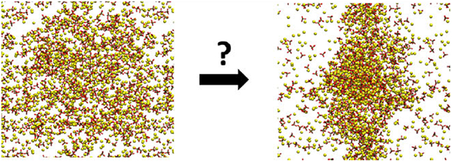
Graphical Abstract

INTRODUCTION

Sodium phosphate salts have a range of stoichiometries and corresponding physical properties related to the multiplicity of charge states that the phosphate group (PO₄³⁻) can take in different chemical situations. Those states can depend on the bonding to other moieties as well as solution or environmental conditions. For the simple sodium salts derived from phosphoric acid the 3 aqueous pK_a values and possible valences dictate stoichiometries for a given condition or state. For biopolymers in aqueous media, most often, either one or two covalent single bonds to the oxygens dictate a charge of −2 or −1, respectively. These are the cases usually found for post-translational protein modifications or for nucleic acid polymers. The charge states and coupled pK_a’s affect many solution properties such as binding and solubilities.

Protein phosphorylation is a fundamental mechanism for cellular signaling that regulates protein function by adding a phosphate group with a −2 charge at a physiological pH near 7. The charge and the excluded volume can alter the structure of the protein and, therefore, its interactions with other proteins.¹ Pathologically, hyperphosphorylation of intrinsically disordered proteins has been shown to be linked to neurodegenerative disease, such as hyperphosphorylation of tau leading to insoluble plaques in Alzheimer’s disease.^2,3 Understanding the effects of phosphorylation on protein behavior is important for studying cellular processes and developing new therapeutics.

However, modeling the solution behavior of phosphorylated proteins using molecular mechanics force fields for subsequent molecular dynamics simulations can be challenging due to the complex interactions between charged species, such as charge transfer and polarization, that can be difficult to account for. This results in known problems where model ions have the tendency to form salt bridges that are more stable than found experimentally.^4,5 This effect becomes especially pronounced at high ionic concentrations.⁶ Locally high effective concentrations, like a high density of charges on the same protein, may have similar effects. A recent study showed that phosphorylated intrinsically disordered proteins (IDPs) tended to be modeled as too compact due to overly stable salt bridges.⁷

The force field parameters for the phosphate group, like most other groups parametrized for simulations, are optimized by fitting to experimental data and/or quantum mechanical calculations at or near infinite dilution.^8,9 The Lorentz–Berthelot (LB) mixing rules,¹⁰ also known as combining rules, are commonly used to estimate Lennard-Jones nonbonded interaction energy well-depth and radius parameters between different types of atoms or particles in molecular simulations. In this simplistic framework, the dispersion energy well-depth parameter between two unlike particles is modeled as the geometric mean of the two, while the radius parameter is the arithmetic mean, which is exact for hard spheres.¹¹ The LB and other mixing rules are a convenience when assuming transferability of the parameters from one molecular situation to another.¹² The assumption that atoms have the same combining rules for the radius and well-depth parameters in every situation is a convenient approximation but not accurate, especially for ions since their charges can strongly affect their interactions with other molecules. The use of LB mixing rules for ions can lead to poor predictions of ion–ion interactions and can limit the accuracy of molecular models of systems involving ionic species. Other nonpolarizable nonbond models for ions such as the Huggins–Mayer form do not suffer from this issue but do not yield simple transferable models for mixing with arbitrary molecules and require each new interaction to be taken as a special case.¹³

To address the issue of over binding by the phosphates in IDPs, one can override a subset of the LB mixing rules with custom parameters fit to experimental data or quantum results. This is a well-known technique used in a variety of simulation and modeling suites, e.g., CHARMM has the nonbonded parameter override, NBFIX.⁶ Currently, the NBFIX radius parameters for sodium and phosphate in the CHARMM force fields were optimized using sodium dimethyl phosphate, a phosphate species with two bridging oxygens and a −1 charge useful for phospholipid and nucleic acid modeling.^14,15 However, these parameters may not accurately represent the behavior of phosphate species with one bridging oxygen and a −2 charge relevant to phosphorylated amino acids and the terminal phosphates in nucleotides.

We take the approach of considering the finite-concentration aqueous solution behavior as a function of the interactions between sodium and phosphate in Na₂HPO₄. We consider the solubility limit of the salt solution as a function of the radius parameters. The Lennard-Jones R_min between phosphate oxygen and sodium will be scanned to allow us to reoptimize the mixing parameter based on experimental solubility data. Note that R_min, used in CHARMM, and van der Waals radius σ are related by R_min = σ × 2^1/6. We will then additionally validate these parameters by calculating the osmotic pressure and comparing it to experimental values, a method previously used to optimize ion interactions.^16,17 By improving the accuracy of the LJ parameters for Na₂HPO₄, we hope to provide a more reliable model for studying the behavior of phosphorylated proteins in future work.

METHODS

We will use molecular dynamics simulations starting from a nonequilibrium supersaturated salt solution to observe the solubility limit after the system phase separates.¹⁸ With a sufficient sample size, the number of molecules left in solution (the “supernatant”) yields an estimate of the solubility limit directly from simulation. With this, we can adjust the Lennard-Jones mixing rules in order to improve the accuracy of the model to fit the solubility of aqueous Na₂HPO₄. Here, we detail the methods that were used.

Solubility Simulation Setup.

We wish to fit Lennard-Jones sodium to phosphate oxygen interaction parameters to match the experimental solubility. There can be two unique species of oxygen in phosphate: nonbridging oxygens (ON3), which carry the bulk of the negative charge, and bridging oxygens (ON4), which carry a smaller negative charge. In HPO₄²⁻, there is one bridging oxygen, which is part of a hydroxyl group, and three nonbridging oxygens (Figure 1). The electrostatic and van der Waals parameters for the phosphate group in nucleic acids and phosphorylated amino acids were initially optimized using monoanionic and dianionic methyl phosphate for CHARMM22;¹⁹ these parameters were carried to CHARMM36. The TIP3P water model was used to be consistent with the CHARMM parameters.²⁰ Since the force field package includes parameters for the phosphate group but not the hydroxyl group in HPO₄²⁻, the charge and LJ parameters for the hydroxyl groups were obtained from the literature (Table 1).²¹

Figure 1.

HPO₄²⁻ ions with CHARMM atom types.

Table 1.

Electrostatic Charge and Lennard-Jones Size and Energy Well-Depth parameters for Different Atom Types in Na₂HPO₄

atom	charge	radius parameter(Rmin/2)	well-depth parameter (ε)
P	1.100	2.15	−0.585
ON3	−0.900	1.70	−0.1200
ON4	−0.730	1.77	−0.1521
HN4	0.330	0.2245	−0.460
SOD	1.000	1.41075	−0.0469

The initial supersaturated configuration of aqueous Na₂HPO₄ was created using a combination of PACKMOL²² and VMD.²³ Using PACKMOL, 625 HPO₄²⁻ were randomly distributed in a cubic box with dimensions of 66 Å on a side. The VMD Solvate plugin was used to randomly distribute TIP3P water molecules around the HPO₄²⁻ in a cubic box with dimensions of 83 Å, where a 17 Å water padding on each side was used to lessen periodic boundary artifacts.²⁴ The VMD Autoionize plugin was used to add 1,250 sodium counterions to neutralize the system, with each ion replacing one water molecule. This resulted in a final count of 12,373 water molecules and a molal concentration for Na₂HPO₄ of 2.8 mol/kg. We note that the molar concentration is adjusted slightly after equilibration (below). The concentration of Na₂HPO₄ was intentionally set to be significantly higher than experimental solubility limit (0.8 mol/kg) as it is less computationally intensive and more accurate to determine the solubility of a solute in the aqueous phase of a supersaturated solution than to sample across multiple concentrations. NAMD was used to run all simulations at constant number, volume, and temperature or the NPT ensemble.²⁵ A 2 fs time step was used. The nonbonded switching function was enabled with a switch distance turned on at 10 Å and off at 12 Å. The pair list distance was set to 14 Å. Rigid bonds were enforced for covalent bonds with hydrogen atoms in the system with a tolerance of 1.0e-8 by using the SHAKE algorithm. A Langevin thermostat was used to control the temperature of the system at 300 K, with a damping coefficient of 0.5. Hydrogen atoms were not coupled to the thermostat. A Langevin piston was used to control the pressure of the system at a target value of 1.01325 bar and a decay time of 100 fs. The piston period was set to 200 fs. The particle-mesh Ewald²⁶ method was used for long-range electrostatic interactions with a real-space grid spacing of 1.0 Å and tolerance of 0.000001.

Solubility Simulation.

In previous studies with NBFIX¹⁵ and CUFIX (Champaign-Urbana NBFIX),¹⁴ only nonbridging oxygens (ON3) were fitted, due to steric effects of bridging oxygens (ON4) limiting sodium interactions. Since the hydroxyl group in HPO₄²⁻ is not sterically hindered, we scan the LJ interatomic distance parameter of both ON3 and ON4 to sodium ions in tandem.

Starting from the same initial configurations, initially, three simulations were run for 40 ns using the following SOD-ON3 LJ interatomic distances: (1) default Lorentz–Berthelot combination rules, (2) NBFIX,¹⁵ and (3) Champaign-Urbana NBFIX.¹⁴ These parameters are summarized in Table 2 under published parameters. The default Lorentz–Berthelot combination rule is the mean of the standard or transferable phosphate oxygen and sodium diameters: R_min (ON3-SOD) = 3.11075 Å. The NBFIX parameter by Luo and Roux takes the LB summation and adds a correction factor to better match the experimental osmotic pressure for dimethyl phosphate: 3.16 Å. The Champaign-Urbana NBFIX parameter uses the same method but used a different correction factor to approximately match the experimental osmotic pressure: 3.20075 Å.

Table 2.

Lennard-Jones Size Parameter Adjustments (ΔR_min) with Simulation Time^b

adjustment (ΔRmin)	Rmin(ON3- SOD)	Rmin(ON4- SOD)	Time (ns)
published parameters
0 (Lorentz–Berthelot)	3.11075	3.16040	40
+0.04925 (NBFIX ON3 only)	3.16	a	40
+0.09 (CUFIX ON3 only)	3.20075	a	40
search parameters
+0.09	3.20075	3.25040	40
+0.115	3.22575	3.27540	400
+0.1213	3.23205	3.28170	278
+0.1275	3.23825	3.28790	600
+0.1338	3.24455	3.29420	322
+0.14	3.25075	3.30040	600
+0.19	3.30075	3.35040	24
curve-fit value
+0.132	3.24275	3.29240	300

^aUnchanged from Lorentz–Berthelot combination rules.

^bNote that ε (ON3-SOD) = −0.075020 and ε (ON4-SOD) = −0.091070 based on Lorentz–Berthelot combination rules (geometric mean) and these are not changed.

During the first 10 ns (nonequilibrium) of simulations, the cubic box dimensions slightly reduced, resulting in a total salt concentration of 2.6M. Whether a phosphate was in cluster or in aqueous solution was defined by whether the heavy atoms of the phosphate were within 4 Å of the largest phase separated cluster. All three simulations rapidly phase separated, forming insoluble clusters with no phosphates remaining in the aqueous phase. The resulting structure from the CUFIX run was then used as an initial condition for subsequent SOD-ON3 and SOD-ON4 optimization. Here, ΔR_min refers to the change of R_min (ON3-SOD) and R_min (ON4-SOD) from the default Lorentz–Berthelot combination rules. The first two simulations adjusted the parameters by ΔR_min = 0.09 and 0.19 Å relative to the LB rules. The next parameters were bisected based on their values relative to experimental solubility. This resulted in the sequence: ΔR_min = 0.14, 0.115, and 0.1275 Å. The ΔR_min = 0.1275 Å correction was close to the experimental solubility of 0.8 mol/kg, two additional values lower and higher than +0.1275 Å were examined, namely, +0.1213 and +0.1338 Å. These results are summarized in Table 2 under the search parameters. The solubility, in molality, was calculated by taking the number of phosphates in solution and dividing it by the mass of the number of water molecules in solution. Water molecules whose oxygens were within 4 Å of the phase separated insoluble clusters were excluded. Finally, the ΔR_min vs solubility fit well to an exponential curve, and the predicted diameter change was found to be ΔR_min, = 0.132 Å. To verify, this value was then simulated for 300 ns, starting from the initial structure as the other simulations, as summarized in Table 2 under the curve-fit parameter. Molality was chosen as the concentration unit as many references reported experimental molal values; these values ranged from 0.77 to 0.86 m.²⁷ However, one source reported both molality and molarity, and they were the same to the first significant digit, namely, 0.84 m and 0.86 M.²⁷ To verify that the molality and molarity are similar in our simulations, molarity was calculated by excluding the volume of the insoluble cluster using the Mol_Volume package.²⁸

Osmotic Pressure Simulation Setup.

We question whether the agreement with the experimental osmotic pressure is consistent for this model with the R_min value found, which reproduces the solubility. The osmotic pressure of a Na₂HPO₄ solution was simulated by using the semipermeable membrane model, where ions are contained within two walls that are permeable to water and impermeable to ions.⁶ The wall setup was adapted from a Tcl script written for NAMD.²⁹ A force constant of 10 kcal/mol/Ų was used for the membranes. Two initial configurations at two concentrations were created: one with 25 Na₂HPO₄ molecules and one with 50 Na₂HPO₄ molecules as a control. As with the solubility simulations, PACKMOL was used to randomly distribute HPO₄²⁻ ions,²² the VMD Solvate plugin was used to add TIP3P waters into the system, and the VMD Autoionize plugin was used to add sodium counterions to neutralize the system. The volume of the initial configuration of the ions was set to 20 × 20 × 20 Å, and the total volume of the initial configuration including water was set to 48 × 48 × 144 Å. The 25 Na₂HPO₄ configuration included 10,226 TIP3P water molecules while the 50 Na₂HPO₄ configuration included 10,030 TIP3P water molecules.

The ion concentration was modulated by changing the membrane separation along the “long” z axis (membrane in the xy plane). For each of the two initial configurations, the z-axis distances between the two membranes were set to 25, 37.5, 50, and 62.5 Å, for a total of 8 systems. The volumes and ionic concentrations for the smaller system are listed in Table 3. The ion concentrations were modulated by changing the membrane separation along the z- axis. Molality was compared against molarity and was shown to be identical within one significant digit.

Table 3.

25 Na₂HPO₄ Ions Simulated in a Box with a Semipermeable Membrane to Calculate the Osmotic Pressure

z axis distance (Å)	volume (nm3)	molarity (mol/L) 25 Na2HPO4	molality (mol/kg) 25 Na2HPO4
25	57.6	0.72	0.71
37.5	86.4	0.48	0.47
50	115.2	0.36	0.36
62.5	144	0.29	0.28

Osmotic Pressure Simulation.

To equilibrate each of the 8 systems, they were each run for at least 30 ns with a time step of 1 fs at NPT. Temperature (300 K) was controlled by Langevin dynamics, and pressure (1.01325 bar) was controlled by a Langevin piston. The dimensions of the x−y plane were kept constant, while the z axis was allowed to fluctuate, so the volume enclosing the ions remains constant. Other details remained the same as those for the solubility simulations. The total volume following 30 ns of equilibration was approximately 48 Å × 48 Å × 130 Å.

Using the equilibration results, each system was run for an additional 30 ns using the NVT ensemble. Osmotic pressure was calculated by measuring the force with which individual ions collide with the two walls averaged across time and divided by the area of the plane. Batch standard error was calculated by dividing each 30 ns trajectory into ten 3 ns blocks. To ensure that the osmotic pressure results depended on concentration and not box size, additional simulations with 50 Na2HPO4 ions at 0.71 mol/kg (with a z-axis distance of 50 Å) were compared against 25 Na₂HPO₄ ions at 0.72 mol/L (with a z-axis distance of 25 Å) and were found to converge to within 1 bar of each other after 30 ns.

Pairwise Correlation Function.

Twenty-five Na₂HPO₄ were placed in aqueous boxes of sizes 57.6 and 144 nm³ to model molal concentrations of 0.28 and 0.71 mol/kg, respectively; R_min = 0.1275 and 0.19 Å. The step size, pressure, and temperature control parameters were the same as the solubility calculations. The pairwise correlation between the oxygen (ON3) in phosphate and sodium was calculated using the VMD g(r) GUI Plugin 1.3. They were averaged over a 35 ns period at 0.01 ns intervals.

Electrostatic and van der Waals Energies.

We wish to check how differences in ΔR_min affected the phosphate interaction energy with other molecules. The electrostatic energy and van der Waals energy of phosphate interactions with other phosphates, sodium, and water were calculated for the 0.28 and 0.71 mol/kg semipermeable simulations across all ΔR_min tested using the VMD NAMD Energy Plugin 1.4. Each simulation was averaged over a 35 ns period at 0.1 ns intervals.

RESULTS

To optimize solubility for Na₂HPO₄, we simulated seven different ΔR_min for phosphate oxygen with sodium (0.09, 0.115, 0.1213, 0.1275, 0.1338, 0.14, and 0.19 Å) and compared the resulting simulated solubility values to experimental solubility. Larger ΔR_min values took longer to equilibrate (Figure S1). All simulations with ΔR_min = 0.1338 Å and below remained a single cluster with a distinct aqueous and cluster phase (representative example shown in Figure 2), while ΔR_min = 0.14 Å and ΔR_min = 0.19 Å broke apart into smaller clusters. We calculated the solubility of Na₂HPO₄ for ΔR_min = 0.14 Å by designating the two largest clusters as being in the cluster phase, while results for ΔR_min = 0.19 Å were not used for the solubility analysis. The clusters have a slow diffusion rate, and we did not need for subclusters to coalesce for this analysis. Overall, the size of the largest cluster, i.e., the insoluble phase, was negatively correlated with ΔR_min (Figure S1). As shown in Figure 3, the solubility of Na₂HPO₄ was found to be exponentially related to ΔR_min, with higher ΔR_min resulting in higher solubility. Among the initially tested parameters, ΔR_min = 0.1275 and 0.1338 Å resulted in solubility limits of 0.5 and 0.9 mol/kg, respectively, which were closest to the experimental solubility limit of 0.8 mol/kg.²⁷

Figure 2.

Snapshot of a Na₂HPO₄ solution with ΔR_min = 0.1275 at 600 ns.

Figure 3.

ΔR_min (size parameter adjustment) and solubility are related exponentially. The experimental solubility is marked with a gray line. The solubility increases by 1 order of magnitude with each 0.027 Å increase. The equation relating ΔR_min and solubility is c_solubility = 9.17 × 10⁻⁶ × e^{86.28 × ΔRmin}. Using 0.8 mol/kg for the experimental solubility limit, ΔR_min was predicted to be 0.132. This parameter was tested, and the result is marked with an asterisk. The standard error of the solubility was smaller than that of the marker.

To determine the optimal fit, we performed a linear regression analysis of ΔR_min versus the logarithm of the simulated solubility. We found the following relationship between ΔR_min and solubility: c_solubility = 9.17 × 10⁻⁶ × e^{86.28 × ΔRmin}. The quality of the fit to an exponential law was excellent, with an R² value of 0.9985. The fit at one extreme predicted a solubility limit of 110 mol/kg for ΔR_min = 0.19 Å, which explains why we were unable to obtain a phase separated cluster starting at 2.8 mol/kg. At the other extreme, the curve predicted a solubility limit of 8.7 × 10⁻⁶ mol/kg for ΔR_min = 0 Å. Using the experimental solubility limit of 0.8 mol/kg, our analysis predicted that the best fit would be achieved with ΔR_min = 0.1320 Å, with a 95% confidence interval between 0.1311 to 0.1328 Å; this resulted in a simulated solubility limit for Na₂HPO₄ predicted to be 0.8 mol/kg, with a corresponding 95% confidence interval of 0.74 to 0.86 mol/kg. A final simulation using ΔR_min = 0.1320 Å revealed that this parameter indeed resulted in a solubility limit statistically indistinguishable from 0.8 mol/kg. A calculation of molarity using the volume of the aqueous phase showed that the molarity and molality were close to equal, consistent with experiments.

Using a single criterion for force field fitting would not ensure accuracy for other properties to be studied subsequently. To validate further the optimized parameters, we calculated the osmotic pressure of Na₂HPO₄ using a subset of the original ΔR_min set (0.09, 0.115, 0.1275, 0.1338, 0.14, and 0.19 as well as the solubility fit of 0.1320, all in units Å) and compared the resulting values to experimental data at 4 concentrations (Table 3). As shown in Figure 4, the simulated osmotic pressures were relatively similar at low concentrations or calculated solubilities across different ΔR_min values and matched the experimental osmotic pressures well. However, at high concentrations of Na₂HPO₄, simulated osmotic pressures for values different from ΔR_min = 0.1320 Å diverged from the experimental values. Corresponding changes in the pair correlation function g(r) are consistent with the general expectations of the Kirkwood–Buff solution theory (Figure 5), although electrostatic and van der Waals energies for phosphates remained similar (Figure S2). ΔR_min = 0.1320 Å, the parameter that provided the best match to experimental solubility limit, also provided the best match to experimental osmotic pressures for various concentrations up to the solubility limit for that model. All models have a range of applicability that generally differs for each independent property to be studied. The validation of the parameters found for solubility limits by testing with calculations of osmotic pressure supports their potential reliability for more than just solubility.

Figure 4.

(Left) Each ΔR_min parameter (0.19, 0.14, 0.1275, 0.115, and 0.09, all in units Å) was run at four different concentrations (0.28, 0.36, 0.47, and 0.71, all in units mol/kg), each for 30 ns. Each open circle indicates a 10 ns average from the 30 ns trajectory, while the plot line passes through the 30 ns average. Osmotic pressures are calculated with the formula Π = icRTϕ, where i is the van’t Hoff factor, c is the concentration, R is the gas constant, T is the temperature, and ϕ is the osmotic coefficient. Osmotic coefficient ϕ is set to 1 for the ideal case; the experimental osmotic coefficient ϕ is obtained from the literature.³⁰ (Right) Osmotic pressure dependence on ΔR_min increases with increasing concentration. Experimental osmotic pressures are marked with horizontal lines. Simulations with ΔR_min = 0.132 Å are marked with asterisks.

Figure 5.

Pair correlation function g(r) of phosphate oxygen (ON3) and sodium is dependent on concentration and ΔR_min. Note that ΔR_min = 0.1275 Å and ΔR_min = 0.19 Å converge with the third coordination shell.

DISCUSSION AND CONCLUSIONS

In this study, we optimized the model Lennard-Jones diameter mixing parameters for phosphate oxygen with sodium for Na₂HPO₄, using experimental solubility data. The resulting parameters were further validated by comparing simulated osmotic pressures to experiments. The solubility was found to be exponentially related to the radius parameter, with roughly every 0.027 Å adjustment resulting in an order of magnitude change in solubility. Our results show that a change from the original parameter of ΔR_min = 0.1320 Å provides the best fit to experimental solubility data, which also fit the experimental osmotic pressure data up to its solubility limit.

The solubility limit is significantly more sensitive to changes in the Lennard-Jones parameters than osmotic pressure. Indeed, ΔR_min = 0.1275 Å and ΔR_min = 0.14 Å, which are approximately equidistant from ΔR_min = 0.132 Å, gave rise to a solubility limit of 0.54 and 1.66 mol/kg, respectively, and osmotic pressures of 28.5 and 32.3 bar at 0.71 mol/kg concentration, respectively. Furthermore, only a relatively narrow range over which R_min-mix parametrization changes osmotic pressure was observed, namely, close to the solubility limit; indeed, there was no statistical difference of osmotic pressure in ΔR_min ranging from 0.115 to 0.19 Å at 0.28 mol/kg (Figure 4) despite significant changes in salt-bridge formation (Figure 5). Therefore, it may be reasonable to parametrize ions to both solubility and osmotic pressure when experimental solubility data for an ion species is available. It is worth noting that the solubility of Na₂HPO₄ is an order of magnitude lower that of NaCl and its molar mass is twice that of NaCl; these are factors that make it more difficult for osmotic pressure to converge but do not affect convergence in solubility-based optimization.¹⁶ Our approach of optimizing parameters based on experimental solubility data and validating them using osmotic pressure calculations may serve as a useful framework for optimizing parameters for other organic and inorganic ions.

Our findings highlight the importance of accurate LJ parameters for simulating the behavior of phosphorylated proteins in phase separating biological systems. Even small adjustments to the diameter mixing parameter can result in significant changes in solubility, spanning several orders of magnitude due to the exponential dependence found. The standard starting parameters for phosphate were optimized using sodium dimethyl phosphate,^14,15 which may be appropriate for nucleic acids and phospholipids but does not accurately represent phosphorylated amino acids at a typical physiological pH due to differences in charge and chemical structure. Under the assumption of potential model transferability, by optimizing the parameters for Na₂HPO₄, we provide a more reliable tool for studying the behavior of phosphorylated proteins. One of the limitations to this study is that it only corrects for phosphate overbinding with the sodium counterion; it does not correct for common interactions with other charged species such as positively charged amino acids or other counterions. Our approach of optimizing parameters based on experimental solubility data and validating them using osmotic pressure calculations may serve as a useful framework for optimizing parameters for other organic and inorganic ions.

REFERENCES

- (1).Nishi H; Hashimoto K; Panchenko AR Phosphorylation in protein-protein binding: effect on stability and function. Structure 2011, 19 (12), 1807–1815. [DOI] [PMC free article] [PubMed] [Google Scholar]
- (2).Noble W; Hanger DP; Miller CCJ; Lovestone S The importance of tau phosphorylation for neurodegenerative diseases. Front. Neurol 2013, 4, 83 DOI: 10.3389/fneur.2013.00083. [DOI] [PMC free article] [PubMed] [Google Scholar]
- (3).Tenreiro S; Eckermann K; Outeiro TF Protein phosphorylation in neurodegeneration: friend or foe? Front. Mol. Neurosci 2014, 7, 42 DOI: 10.3389/fnmol.2014.00042. [DOI] [PMC free article] [PubMed] [Google Scholar]
- (4).Tolmachev DA; Boyko OS; Lukasheva NV; Martinez-Seara H; Karttunen M Overbinding and Qualitative and Quantitative Changes Caused by Simple Na+ and K+ Ions in Polyelectrolyte Simulations: Comparison of Force Fields with and without NBFIX and ECC Corrections. J. Chem. Theory Comput 2020, 16 (1), 677–687. [DOI] [PubMed] [Google Scholar]
- (5).Vymětal J; Jurásková V; Vondrášek J AMBER and CHARMM Force Fields Inconsistently Portray the Microscopic Details of Phosphorylation. J. Chem. Theory Comput 2019, 15 (1), 665–679. [DOI] [PubMed] [Google Scholar]
- (6).Luo Y; Roux B Simulation of Osmotic Pressure in Concentrated Aqueous Salt Solutions. J. Phys. Chem. Lett 2010, 1 (1), 183–189. [Google Scholar]
- (7).Rieloff E; Skepö M Molecular Dynamics Simulations of Phosphorylated Intrinsically Disordered Proteins: A Force Field Comparison. Int. J. Mol. Sci 2021, 22 (18), 10174 DOI: 10.3390/ijms221810174. [DOI] [PMC free article] [PubMed] [Google Scholar]
- (8).Feng M-H; Philippopoulos M; MacKerell AD Jr.; Lim C Structural Characterization of the Phosphotyrosine Binding Region of a High-Affinity SH2 Domain–Phosphopeptide Complex by Molecular Dynamics Simulation and Chemical Shift Calculations. J. Am. Chem. Soc 1996, 118 (45), 11265–11277. [Google Scholar]
- (9).Denning EJ; Priyakumar UD; Nilsson L; Mackerell AD Impact of 2’-hydroxyl sampling on the conformational properties of RNA: update of the CHARMM all-atom additive force field for RNA. J. Comput. Chem 2011, 32 (9), 1929–1943. [DOI] [PMC free article] [PubMed] [Google Scholar]
- (10).Hansen JP; McDonald IR Theory of Simple Liquids; Academic Press: London: 1976. [Google Scholar]
- (11).MacKerell AD; Bashford D; Bellott M; Dunbrack RL; Evanseck JD; Field MJ; Fischer S; Gao J; Guo H; Ha S; et al. All-atom empirical potential for molecular modeling and dynamics studies of proteins. J. Phys. Chem. B 1998, 102 (18), 3586–3616, DOI: 10.1021/jp973084f. [DOI] [PubMed] [Google Scholar]
- (12).Jorgensen WL Transferable Intermolecular Potential Functions for Water, Alcohols, and Ethers. Application to Liquid Water. J. Am. Chem. Soc 1981, 103, 335–340. [Google Scholar]
- (13).Pettitt BM; Rossky PJ Alkali halides in water: Ion–solvent correlations and ion–ion potentials of mean force at infinite dilution. J. Chem. Phys 1986, 84 (10), 5836–5844. [Google Scholar]
- (14).Yoo J; Aksimentiev A Improved Parametrization of Li+, Na+, K+, and Mg2+ Ions for All-Atom Molecular Dynamics Simulations of Nucleic Acid Systems. J. Phys. Chem. Lett 2012, 3 (1), 45–50. [Google Scholar]
- (15).Venable RM; Luo Y; Gawrisch K; Roux B; Pastor RW Simulations of anionic lipid membranes: development of interaction-specific ion parameters and validation using NMR data. J. Phys. Chem. B 2013, 117 (35), 10183–10192. [DOI] [PMC free article] [PubMed] [Google Scholar]
- (16).Luo Y; Roux B Simulation of Osmotic Pressure in Concentrated Aqueous Salt Solutions. J. Phys. Chem. Lett 2010, 1 (1), 183–189. [Google Scholar]
- (17).Lin FY; Huang J; Pandey P; Rupakheti C; Li J; Roux BT; MacKerell AD Jr. Further Optimization and Validation of the Classical Drude Polarizable Protein Force Field. J. Chem. Theory Comput 2020, 16 (5), 3221–3239. [DOI] [PMC free article] [PubMed] [Google Scholar]
- (18).Karandur D; Wong K-Y; Pettitt BM Protein Folding and Collapse: Thermodynamics of Aggregation of Gly5 vs Concentration in Solution. Biophys. J 2014, 106 (2 Supplement 1), 483a. [Google Scholar]
- (19).MacKerell AD Jr.; Widrkiewicz-Kuczera J; Karplus M An all-atom empirical energy function for the simulation of nucleic acids. J. Am. Chem. Soc 1995, 117 (48), 11946–11975. [Google Scholar]
- (20).Jorgensen WL; Chandrasekhar J; Madura JD; Impey RW; Klein ML Comparison of simple potential functions for simulating liquid water. J. Chem. Phys 1983, 79 (2), 926–935. [Google Scholar]
- (21).Yang Y; Cui Q; Sahai N How does bone sialoprotein promote the nucleation of hydroxyapatite? A molecular dynamics study using model peptides of different conformations. Langmuir 2010, 26 (12), 9848–9859. [DOI] [PubMed] [Google Scholar]
- (22).Martínez L; Andrade R; Birgin EG; Martínez JM PACKMOL: a package for building initial configurations for molecular dynamics simulations. J. Comput. Chem 2009, 30 (13), 2157–2164, DOI: 10.1002/jcc.21224. [DOI] [PubMed] [Google Scholar]
- (23).Humphrey W; Dalke A; Schulten K VMD: visual molecular dynamics.J. Mol. Graphics 1996, 14 (1), 33–38, DOI: 10.1016/0263-7855(96)00018-5. [DOI] [PubMed] [Google Scholar]
- (24).Workman RJ; Pettitt BM Thermodynamic Compensation in Peptides Following Liquid-Liquid Phase Separation. J. Phys. Chem. B 2021, 125 (24), 6431–6439, DOI: 10.1021/acs.jpcb.1c02093. [DOI] [PMC free article] [PubMed] [Google Scholar]
- (25).Phillips JC; Hardy DJ; Maia JDC; Stone JE; Ribeiro JV; Bernardi RC; Buch R; Fiorin G; Hénin J; Jiang W; et al. Scalable molecular dynamics on CPU and GPU architectures with NAMD. J. Chem. Phys 2020, 153 (4), No. 044130, DOI: 10.1063/5.0014475. [DOI] [PMC free article] [PubMed] [Google Scholar]
- (26).Darden T; York D; Pedersen L Particle mesh Ewald: An N · log(N) method for Ewald sums in large systems. J. Chem. Phys 1993, 98, 10089–10092. [Google Scholar]
- (27).Eysseltova J. Disodium Hydrogen Phosphate. IUPAC Solubility Data Series 1988, 31, 103–106. [Google Scholar]
- (28).Balaeff A. Mol_Volume. [Google Scholar]
- (29).de Souza RM; Romeu FC; Ribeiro MCC; Karttunen M; Dias LG Osmotic Method for Calculating Surface Pressure of Monolayers in Molecular Dynamics Simulations. J. Chem. Theory Comput 2022, 18 (4), 2042–2046. [DOI] [PubMed] [Google Scholar]
- (30).Goldberg RN Evaluated activity and osmotic coefficients for aqueous solutions: thirty-six uni-bivalent electrolytes. J. Phys. Chem. Ref. Data 1981, 10 (3), 671–764. [Google Scholar]
Associated Data
This section collects any data citations, data availability statements, or supplementary materials included in this article.