

Abstract
The short association fibers or U-fibers travel in the superficial white matter (SWM) beneath the cortical layer. While the U-fibers play a crucial role in various brain disorders, there is a lack of effective tools to reconstruct their highly curved trajectory from diffusion MRI (dMRI). In this work, we propose a novel surface-based framework for the probabilistic tracking of fibers on the triangular mesh representation of the SWM. By deriving a closed-form solution to transform the spherical harmonics (SPHARM) coefficients of 3D fiber orientation distributions (FODs) to local coordinate systems on each triangle, we develop a novel approach to project the FODs onto the tangent space of the SWM. After that, we utilize parallel transport to realize the intrinsic propagation of streamlines on SWM following probabilistically sampled fiber directions. Our intrinsic and surface-based method eliminates the need to perform the necessary but challenging sharp turns in 3D compared with conventional volume-based tractography methods. Using data from the Human Connectome Project (HCP), we performed quantitative comparisons to demonstrate the proposed algorithm can more effectively reconstruct the U-fibers connecting the precentral and postcentral gyrus than previous methods. Quantitative validations were then performed on post-mortem MRIs to show the reconstructed U-fibers from our method more faithfully follow the SWM than volume-based tractography. Finally, we applied our algorithm to study the parietal U-fiber connectivity changes in autosomal dominant Alzheimer’s disease (ADAD) patients and successfully detected significant associations between U-fiber connectivity and disease severity.
Index Terms—: Tractography, Superficial white matter, U-fibers
I. INTRODUCTION
Superficial white matter (SWM) lies directly beneath the cortex and contains the short association fibers, or U-fibers, connecting neighboring gyri [1–3]. Over the last decade, significant advances have been made in connectome imaging techniques with dramatically increased spatial and angular resolution in diffusion MRI (dMRI) [4]. Current connectome research, however, focuses primarily on long-range fiber connections in the deep white matter (DWM) with little attention paid to the U-fibers in the SWM even though the SWM has approximately twice as many fiber connections as the DWM [5] and plays an essential role in various brain disorders [6–9]. In this work, we will develop a novel fiber tracking framework based on the surface representation of the SWM and provide dedicated tractography tools for modeling U-fiber connectivity.
Tractography based on dMRI is the most widely used method for reconstructing fiber connections in the human brain in vivo. Popular tractography methods typically realize tracking via sampling and interpolating a fiber trajectory through the 3D image grid of the dMRI based on various mathematical representations about fiber distributions within voxels [10, 11]. Previous works on fiber tracking in SWM primarily rely on existing tractography methods. For example, cortical ROIs were used to select fiber tracts for specific bundles of U-fibers [12–16]. In addition, whole-brain tractography was applied to cluster U-fibers throughout the cortex [17–20] and to construct atlases [21]. One known limitation of existing volume-based tractography methods is that they tend to have a large number of false negatives in the reconstruction of highly curved fibers, such as the U-fibers [22]. Previous tractography methods can thus typically only provide a partial representation of the U-fiber connections in the SWM.
There has been increasing interest in advancing the tracking of U-fibers by leveraging the surface representation of the SWM. A surface-based seeding approach was proposed recently to enhance the reconstruction of U-fibers [23], but it still relies on conventional volume-based tractography for fiber tracking and cannot prevent the reconstructed tracts from deviating away from the sheet-like structure of the SWM. To ensure the U-fibers follow the SWM beneath the cortex, we proposed a surface-based tractography method [24] that tracks the U-fibers on the triangular mesh representation of the SWM. This deterministic tracking approach follows the peaks of the interpolated fiber orientation distribution (FOD) [10] on the SWM mesh to generate the U-fibers. This method outperforms volume-based tractography in reconstructing U-fibers that connect the precentral and postcentral gyrus. While this method performs tracking on a triangular mesh, it has not fully utilized the intrinsic surface geometry of the SWM to avoid limitations in existing volume-based tracking. For example, it relies on angular differences from R3 in quantifying the changes of directions during the tracking propagation process and hence does not follow the intrinsic surface geometry to regularize tract smoothness. In addition, the deterministic tracking approach does not consider the uncertainty in fiber orientations and can affect the completeness of U-fibers’ reconstruction.
In this work, we will develop a novel surface-based probabilistic tracking framework for reconstructing U-fibers in SWM. Our method systematically tackles challenges in existing volume- and surface-based methods for U-fiber tracking. First, we carefully generate the surface representation of SWM based on nonlinear registration and deformation of the white matter (WM) surface computed from T1-weighted MRI. After that, we develop a novel method to project the 3D FODs onto the tangent space of the SWM surface based on an efficient transformation of spherical harmonics (SPHARM) representation of FODs to the local coordinate system of the tangent space. A probabilistic tracking method is then developed based on the projected 2D FODs on the SWM surface, where parallel transport is adopted to propagate the streamlines across triangles and regularize tract smoothness intrinsically. By tracking based on the intrinsic geometry of the SWM surface, our method avoids the sharp turning angles of SWM in the 3D space and can significantly improve the reconstruction of U-fibers in the SWM. In our experiments, we demonstrate that our proposed method achieves superior performance than previous tracking algorithms on both in vivo and post-mortem human connectome imaging data. Furthermore, we applied our method to study SWM connectivity changes in autosomal dominant Alzheimer’s disease (ADAD) patients and demonstrated statistically significant associations between parietal U-fiber connectivity and disease severity. An open-source implementation of the proposed method is distributed freely to the research community (https://github.com/Xinyu-Nie/SurfTracker).
The rest of the paper is organized as follows. In section II, we present the novel surface-based probabilistic tracking method, including the surface representation of the SWM, efficient calculation of the 2D FOD projections, and the probabilistic fiber tracking on the SWM surface. Experimental results on three datasets are presented in section III. Finally, discussions and conclusions are in section IV.
II. Method
A. Mesh Representation of SWM
The proposed novel method for tracking the U-fibers is based on the surface representation of the SWM, so the accurate placement of the cortical surfaces in the diffusion MRI (dMRI) space is a prerequisite. As a first step, the triangular mesh representation of the white matter (WM) and gray matter (GM) cortical surfaces are reconstructed from the T1-weighted MRI by FreeSurfer [25, 26]. For the dMRI data, we apply the HCP-Pipeline [27] for distortion correction and its registration with the T1-weighted MRI. Nonlinear distortions, however, still exist after these processes and affect the accurate alignment of cortical surfaces with dMRI (Fig.1. (c)). To remove the residual misalignment, we compute the compartment models from the multi-shell dMRI by our previous work [10], which generates a diffusivity map (Fig.1. (b)) of the extra-axonal compartment for nonlinear registration with the T1-weighted MRI (Fig.1. (a)) by the ANTS software [28]. After that, we apply the nonlinear deformation calculated by ANTS to transform the WM surface from the T1-weighted MRI to the space of the dMRI, which aligns more accurately with the tissue boundaries, as shown in Fig.1. (d). Finally, the transformed WM mesh is deformed inward toward the deep white matter (DWM) along the normal direction by a distance of δ (e.g., 0.5mm) to generate the SWM mesh for surface-based fiber tracking.
Fig. 1.

Accurate placement of the WM cortical surface in the dMRI space. (a) T1-weighted MRI; (b) the extra-axonal diffusivity calculated from dMRI by our compartment models. After the preprocessing by HCP-Pipeline, yellow arrows in (c) highlight the residual misalignment of the WM cortical surface (cyan) and the intra-axonal tissue map calculated by our compartment models. (d) shows the much-improved alignment of the WM cortex (green) with the same tissue map after nonlinear registration between T1-weighted MRI in (a) and the extra-axonal diffusivity map in (b).
B. FOD Projection onto SWM Surface
The fiber orientation distribution (FOD) represents complicated fiber configurations as a function on a unit sphere and has been used widely for fiber tracking in the 3D space. Since we track the U-fibers on the surface rather than R3, the whole tracking procedure must be presented in the surface’s local coordinates and tangent spaces. Thus, we represent the 3D FOD, which we denote as FOD3D, in the surface’s local coordinates and project the FOD3D onto the tangent space of the SWM surface. For this purpose, we will first construct a local spherical coordinate system at each triangle (tangent space) of the SWM mesh, as shown in Fig.2. (a), where the normal of the triangle is the zenith direction, an edge of the triangle is chosen as the x-axis whose azimuthal angle φ equals 0, and the polar angle θ is the angle with respect to the zenith direction. Fig.2. (a) shows a FOD3D function at the center of a triangle on the SWM mesh, and it is projected onto the triangle plane as a FOD2D function in Fig.2. (b). In this local coordinate system, we parameterize the 3D FOD as FOD3D(θ,φ) and project it onto the tangent space as:
| (1) |
Fig. 2.

The projection of 3D FODs onto 2D triangles local coordinate systems. (a) The FOD3D function is represented in a local spherical coordinate system defined on the center of a triangle of the SWM mesh. The reference plane of the system is the triangle plane, meanwhile the zenith direction z is aligned with the normal direction. The x-axis is aligned with an edge of the triangle. (b) The projected FOD2D using the formula (1). The FOD2D function is parametrized by φ in the local coordinate system and can be normalized to a probability distribution function on the unit circle S1.
The projected FOD2D function is parametrized by the azimuth angle φ in the local coordinate system and defined on a unit circle S1 in the tangent space of the SWM surface, as shown in Fig.2. (b). The weighted term sin(θ) in integral (1) reduces the diffusion information perpendicular to the SWM surface. The integral of the FOD2D function on the circle equals the integral of the FOD3D function on the sphere.
On the other hand, 3D FOD at each voxel is commonly parameterized by the spherical coordinates in the physical space of the MRI scans. In addition, the FOD is often represented by the coefficients of real spherical harmonics (SPHARM), up to an order N:
| (2) |
where is the m-th (-n≤m≤n) real SPHARM at the order n (0≤n≤ N) and is the coefficient for the corresponding basis; θ0 and φ0 are the polar and azimuth angles of the spherical coordinates in the space of the MRI scan in R3; and are normalization constants; is the associated Legendre polynomial at degree n and order m. The SPHARM functions form an orthonormal basis on the unit sphere and perform similarly to the Fourier Series on the unit circle.
A critical challenge to track the U-fibers based on the projected FOD2D in the surface’s local coordinate system, as described in formula (1), is to efficiently obtain the SPHARM representation of FOD3D in the local spherical coordinate system, i.e., we need to solve for the SPHARM coefficients at each triangle:
| (3) |
where is the unknown coefficient for the real SPHARM basis in the local system and is the given coefficient in the standard physical coordinate system as in (2); (θ0,φ0) and (θ,φ) represent the same point in the different coordinates as in Fig.3. With the SPHARM representation of FODs in the local spherical coordinate system, we can write (1) as:
| (4) |
Fig. 3.

The local coordinate system Oxyz differs from the physical coordinate system Ox0y0z0 by a rotation R. (θ0,φ0) and (θ,φ) represent the same point p in the two systems. The rotation R is decomposed as three successive rotations around three axes: (a) Ox0y0z0 is rotated by an angle α around Oz0 → Ox1y1z0; (b) Ox1y1z0 is rotated by a second angle β around Oy1 → Ox2y1z2; (c) Ox2y1z2 is rotated by a third angle γ around Oz2 → Ox3y3z2, which is Oxyz.
The integrals in equation (4) are independent of the data and can be precomputed at a high level of numerical precision; thus, we can accurately calculate the FOD2D function using (4) with very small computational costs given the SPHARM coefficients of FOD3D in the local coordinate system.
The key to computing from is to represent by a linear combination of ; namely, find the transformation of SPHARMs under a coordinate system rotation. Since it is much easier to derive the rotation transformation for complex SPHARMs, we first transform the real SPHARM representation of FOD3Ds into complex SPHARMs and then derive the rotation transformation between two coordinate systems based on the complex SPHARMs. After that, the results will be transformed back to the real SPHARM representation to obtain the final form for numerical calculation. The m-th (-n≤m≤n) complex SPHARM at the order n is:
| (5) |
where is a normalization constant. The basis transfer from real to complex SPHARMs is:
| (6) |
where is the m-th real SPHARM basis at the order n, and is the m-th complex SPHARM basis at the order n. This basis transfer is invertible, and its inverse is:
| (7) |
We denote the transfer in (6) as a matrix U and its inverse (7) as U−1, respectively.
For a rotation R from the coordinate system Ox0y0z0 (Fig.3) of the MRI physical space to the local coordinate system Oxyz of the current triangle, we follow Wigner’s work [29] to decompose it as three successive rotations around three axes: (a) Ox0y0z0 is rotated by an angle α around Oz0 → Ox1y1z0; (b) Ox1y1z0 is rotated by a second angle β around Oy1 → Ox2y1z2; (c) Ox2y1z2 is rotated by a third angle γ around Oz2 → Ox3y3z2, which is Oxyz. The angles (α, β, γ) are the Euler angles, where α is computed by finding the angle between Oy and the cross product of Oz and Oz0, β is the angle between Oz and Oz0, and γ is the angle between Ox and Ox2 in step (c) above. In the following, we represent the successive operations in the order from right to left, and the rotation R operator is now:
| (8) |
where Zγ is the rotation around the z-axis in the current coordinate system by an angle γ as explained above, and the other two operators are similarly defined.
Based on a group symmetry argument [29], Wigner has proven that Wigner D-matrices can represent the transformation of the n-th order complex SPHARMs between two coordinate systems based on the decomposition in (8):
| (9) |
where Wn is a (2n+1) complex vector that represents the n-th order complex SPHARMs; Dn is a (2n+1)-by-(2n+1) matrix:
| (10) |
where the first and third terms correspond to the rotations Zα and Zγ in (8), and the middle term is induced from the rotation Yβ. The rotation around the z-axis is trivial since it only changes the azimuth angle φ in the complex SPHARMs. The term , which corresponds to a rotation around the y-axis, is much more challenging to handle. Wigner showed that the rotation Yβ could be decomposed into successive rotations as:
| (11) |
Combining equations (8) and (11), we have:
| (12) |
The decomposition in (12) is much easier to compute since the rotations that depend on angles (α, β, γ) are around the z-axis; meanwhile, the difficult rotations around the y-axis are fixed, π/2 or -π/2. The closed-form solution [30, 31] of is:
| (13) |
where P is the Jacobi polynomial, and other elements of this (2n+1)-by-(2n+1) matrix can be induced by the symmetric properties [30, 31]. We can now decompose the matrix Dn(α,β,γ) in equations (9) and (10) as successive matrices:
| (14) |
where and represent the matrix dn in equation (13) at β = -π/2 and π/2; is the diagonal matrix induced from the rotation by an angle ω around the z-axis. Let vn and un represent the coefficients of the n-th order real SPHARMs under the local coordinate system at the current triangle and standard coordinate system of the MRI scan; we have the following formula based on equations (4), (6), (7), and (9):
| (15) |
where U and U−1 come from (6) and (7); vn is a real (2n+1) vector whose m-th element is in (3), and un is the vector of real SPHARM coefficients in (3).
With the transformation of the real SPHARM coefficients from the common physical space to the local coordinate system on each triangle, we can represent the FOD3D function using the real SPHARMs in the local system and compute its 2D projection according to equation (4). Each FOD2D function is defined on a triangle plane and represents the diffusion propagation information within this triangle, which allows us to track the U-fibers on the SWM mesh probabilistically.
C. Parallel Transport
Streamlining-based tractography methods typically regularize the smoothness of fiber tracts by controlling the angular difference of consecutive tracking directions. However, for surface-based tracking of SWM, a direct angle comparison in R3 is not meaningful since the track’s previous direction and new sampling direction lie in different tangent spaces of the surface. To incorporate a regularization mechanism consistent with the surface geometry of the SWM, we develop an intrinsic approach to compare tracking directions based on the parallel transport of vectors on surfaces.
An affine connection (or covariant derivative) introduces a geometric structure on a manifold to compare vectors in neighboring tangent spaces [32]. Since the SWM mesh is embedded in R3, the Levi-Civita connection induced by the Riemannian metric can be naturally used. With the Levi-Civita connection, a vector in a tangent space can be parallel transported (the covariant derivative along the path is 0) to another tangent space as in Fig.4; namely, the parallel transported vector uγ(t) along a curve satisfies the following differential equations:
| (16) |
where ∇ is the Levi-Civita connection, γ(t) is a curve connecting point p and point q; uγ(t) is the parallel transported vector along the curve. This differential equation system always has a unique solution by the existence and uniqueness theorem of differential equations if the point q is close to the point p.
Fig. 4.

For a vector up in the tangent space of point p on a Riemannian manifold, the Levi-Civita connection parallel transports up along a geodesic γ(t) to a vector uq in the tangent space of point q, which allows the comparison of vectors in the tangent spaces of nearby points.
For a track that leaves a current triangle and enters an adjacent triangle, we will parallel transport the tracking direction in the current triangle to the new triangle to allow the comparison of angular differences during the tracking process for smoothness regularization. The parallel transport induced by the Levi-Civita connection can be numerically realized for two adjacent triangles on the SWM mesh, as shown in Fig.5; namely, the parallel transport is achieved by unfolding the pair of adjacent triangles, translating the vector from one triangle to the other along the geodesic (straight line) in the unfolded plane, and finally folding the triangles back to their original positions together with the transported vector [33]. Since we use the projected FOD2D function on each triangle for the sampling of fiber tracking directions, we express the parallel transport based on the local spherical coordinate system of each triangle. For a direction v parametrized by the azimuth angle φ in the local coordinate system of a triangle T1, as in Fig.5. (a), the vector v is represented as:
| (17) |
where ex and z are the directional vectors of the x-axis edge and normal in T1 as illustrated in Fig.5, and the matrix R is the operator that rotates by angle φ around the normal direction z. The parallel transport from a triangle T1 into T2 is achieved by rotating the vector v as follows:
| (18) |
where ec is the directional vector of the shared edge of T1 and T2, and θc is the angle between the normal vectors of the two triangles (the two triangles must be oriented in the same way). The vector vp lies in the plane of triangle T2 and can be compared with any newly sampled direction in triangle T2, as in Fig.5. (c), for the calculation of intrinsic angular differences during the fiber tracking process.
Fig. 5.

The parallel transport of a vector v in the current triangle T1 to a neighboring triangle T2. The parallel transport consists of unfolding the triangles to a common plane (a)~(b), translating the red tangent vector v from T1 to T2 (b), and folding the triangles back to their original positions (b)~(c). The transported vector vp can then be compared with any sampling direction w in the triangle T2.
In the extreme case where a track leaves the current triangle at a vertex vi instead of any edge, we use the geodesic polar map [34] to flatten all triangles in the one-ring neighborhood of the vertex into a 2D chart. The geodesic polar map of the vertex vi flattens its one-ring neighborhood into a plane by enforcing the geodesics from vi (i.e., lines starting at vi) to remain straight in the plane while rescaling the angles between geodesics by:
| (19) |
where θjik is the angle at the vertex vi of all triangle Tjik in the one-ring neighborhood of vi. In the 2D chart, we can easily find the upcoming triangle to continue the tracking by extending the tracking line through the vertex. Finally, we map the extended tracking line from the 2D chart to the original position of the upcoming triangle in the 3D mesh by the inverse geodesic polar map, which will be the parallel transported vector to compare the angular difference between tracking directions of neighboring triangles.
Algorithm 1.
Surface-based Probabilistic Tractography
| Inputs: FODs, WM mesh, seed ROI, stopping condition, deformation distance δ, angle threshold θin, FOD2D cut-off threshold FODmin. |
| Output: N U-fibers on the SWM mesh. |
|
D. Tracking Algorithm
Using the triangular mesh representation of SWM and projected FOD2Ds, we will develop a surface-based probabilistic fiber tracking algorithm of U-fibers as listed in Algorithm 1. Our algorithm starts from a randomly selected seed triangle and propagates a streamline on the SWM mesh until a user-defined stopping condition is met. Similar to previous FOD-based tractography algorithms, the stopping condition can be: (a) the streamline arrives at the boundary of a predefined mask on the SWM mesh; (b) the streamline meets the conditions of including or excluding ROIs from user-defined protocols; (c) no valid FOD2D data to continue the tracking. In Algorithm 1, Tn denotes a triangle from the triangular mesh, pn denotes a point of the streamline, NT denotes the neighboring triangles of a triangle T, and T denotes the boundary of the triangle T. The Main steps of Algorithm 1 are explained as follows.
Sampling:
For a point pn and the triangle Tn, the rejection sampling method is used to sample the direction of the streamline based on the normalized FOD2D function of the triangle Tn. No smoothness regularization is needed for the sampled direction when pn is the seed point. In other cases, we repeat sampling the direction until the angle difference between the sampled direction v and the parallel transported vector vp is less than a threshold θin. Moreover, the FOD2D value of the sample direction v is required to exceed a threshold FODmin to reduce the propagations in areas with a low probability of valid fiber connections. If there is no accepted direction until the sampling times reach a threshold (e.g., 50), we abort the current fiber tracking process and restart it from a newly sampled seed triangle.
Propagation within a triangle:
For the point pn within the triangle Tn (including the boundary points), we compute a line segment to propagate the streamline piecewise linearly, which originates from pn and terminates at the triangle boundary following the sampled direction v. Then the terminating point p enters an adjacent triangle T and act as the start point of the next line segment in this new triangle.
Propagation across triangles:
When our streamline leaves a current triangle and enters one adjacent triangle, we parallel transport the direction v in the current triangle to vp that lies in the new triangle using the method in section II.C. The vector vp is used for smoothness regularization, as discussed in the rejection sampling process.
In Algorithm 1, we apply the fiber tracking in symmetric directions at a seed triangle. After completing tracking in both directions, we concatenate the two streamlines to form a complete U-fiber on the SWM mesh. For practical U-fiber tracking experiments, the user needs to specify the seed ROIs and properly define the stopping criteria on the cortical surface. We will give more detailed examples of setting up surface-based tracking protocols in our experimental results.
III. Experiments and Results
We will apply our surface-based fiber tracking algorithm to three datasets to demonstrate its effectiveness in reconstructing U-fibers in the SWM. We first apply the proposed method to the high-resolution dMRI data from the Human Connectome Project (HCP) [35] and compare it with two other tractography methods. After that, we apply our method to two post-mortem scans and validate the agreement between the tracked U-fibers and manually delineated SWM from their high iron contrast on T2-weighted MRI. Finally, we apply our method to reconstruct the U-fibers in the parietal lobes of 26 subjects with ADAD and show that a significant association of U-fiber connectivity with disease severity can be successfully detected.
A. U-fiber Tracking on HCP Subjects
In our first experiment, the T1-weighted MRI and multi-shell dMRI data of 484 subjects from the HCP 500 Subject Release were used. The age range of the 484 subjects is 22 to 36 years old, and there are 195 males and 289 females. T1-weighted MRI of HCP has an isotropic resolution of 0.7mm, and dMRI images have an isotropic resolution of 1.25mm and were acquired from 270 gradient directions distributed over three different b-values: 1000, 2000, and 3000 s/mm2. All data were first preprocessed by version 3 of the HCP-Pipeline, which reconstructs the cortical surfaces from the T1-weighted MRI and registers the dMRI to the T1-weighted MRI after artifact correction. After that, FODs and compartmental parameters were computed [10]. In this experiment, we will reconstruct the U-fibers connecting the pre- and post-central gyrus [12, 14, 18] and compare the performance with state-of-the-art volume-based fiber tracking from the MRtrix software [36] and a deterministic surface-based fiber tracking method [24] that our group developed previously.
As the first step for surface-based tracking, we resampled the WM cortical surface from the left hemisphere of all subjects into a mesh with 20,000 triangles and deformed it toward the DWM along the normal direction by a distance of δ=0.5mm, which will be validated in our second experiment for the generation of the SWM mesh in surface-based tracking. Following the work in [24], we used the Hamilton-Jacobi skeleton method [37] to generate the gyral skeletons of the pre-and post-central gyrus according to FreeSurfer labels. The gyral skeletons from these two gyri will be used as the inclusion ROIs for surface-based tracking. The stopping condition for surface-based tracking is that both inclusion ROIs have been reached. Furthermore, the seed ROI for surface-based tracking is obtained as triangles within a 2mm geodesic distance to the boundary between the pre- and post-central gyrus. For the MRtrix software, all neighboring voxels of the triangles in the seed ROI on the SWM mesh are combined to form the seed ROI in volume-based fiber tracking. The gray and white matter masks of the pre- and post-central gyrus from the aseg results of FreeSurfer were combined to form the mask for fiber tracking with MRtrix, which will stop the tracking if a tract leaves the mask.
For the deterministic surface-based method in [24], we set the step size to be 0.01mm, the two angle thresholds as THθin = 1 degree and THθxing = 10 degrees, as used in the same experiment in [24]. For the proposed novel probabilistic surface-based fiber tracking method, we set the angle threshold θin = 10 degrees and the FOD2D cut-off threshold FODmin = 0.01. The iFOD1 algorithm was used for MRtrix, and the main parameters of iFOD1 were set as step size = 0.1mm, angle threshold = 10 degrees, and the FOD3D cut-off threshold used for the MRtrix was 0.05. For all methods, 30,000 seed points were randomly sampled for fiber tracking.
Reconstructed U-fibers from five representative HCP subjects are shown in Fig.6. For all subjects, U-fibers reconstructed by the volume-based tractography in MRtrix do not closely follow the cortical folding, and most streamlines do not touch the gyral skeletons. On the other hand, both surface-based methods can generate U-shaped streamlines that follow tightly to the cortical surface. Compared to the surface-based deterministic method, the proposed probabilistic and surface-based fiber tracking method provides more geometrically regular and topographically organized U-fibers connecting the two neighboring gyri.
Fig. 6.
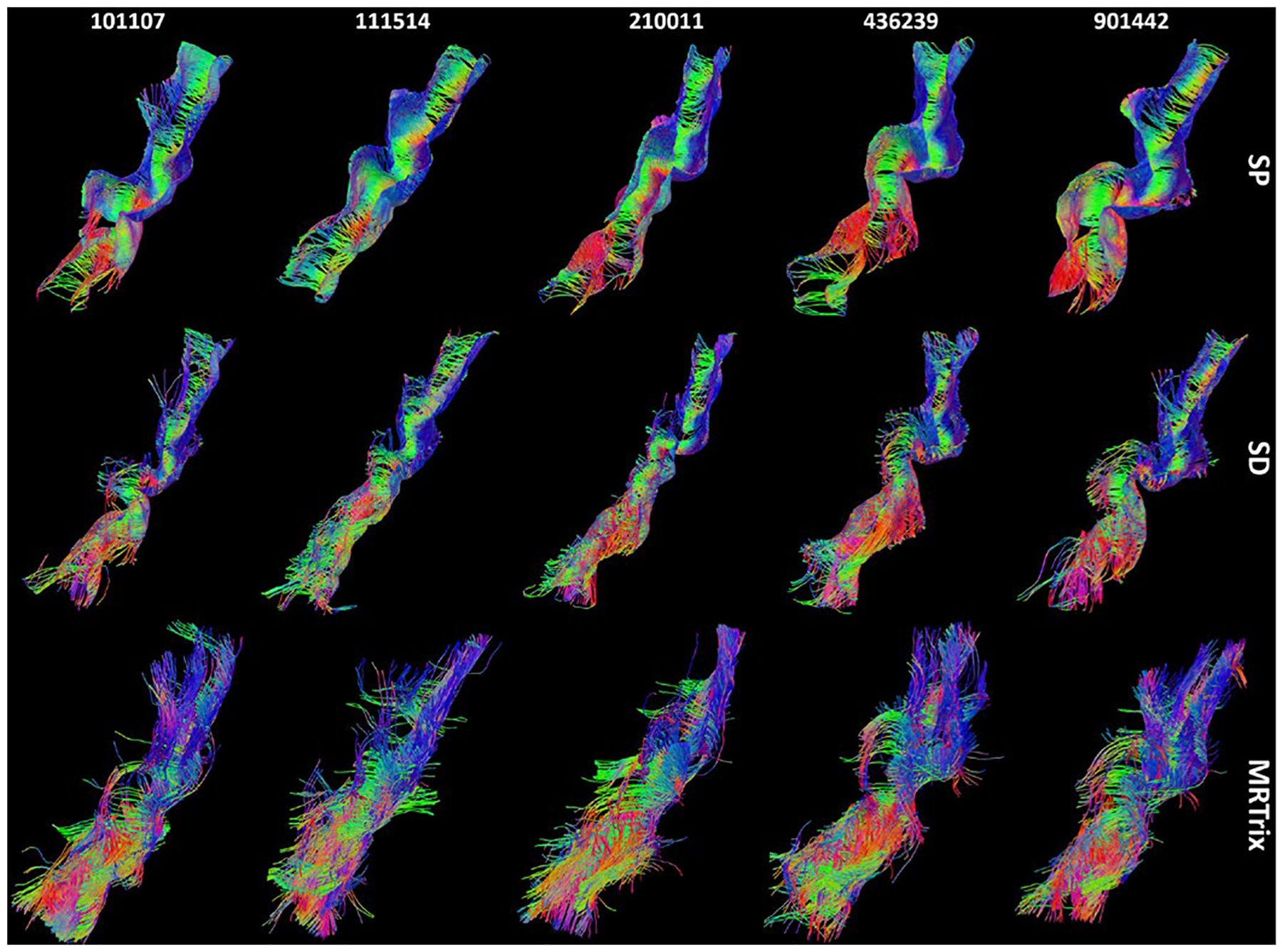
Representative HCP examples of U-fibers between the pre- and post-central gyrus reconstructed by the two surface-based methods (SP: surface-based probabilistic tracking; SD: surface-based deterministic tracking) and the MRtrix software. For better visualization, we downsampled all results to 1000 streamlines. The subject ID is plotted at the top of the results from each HCP subject.
To quantitatively evaluate the performance of the fiber tracking methods in the reconstruction of U-fibers in SWM, we use three similar measures proposed in [24]: ‘well-U-connected’, ‘well-distributed’, ‘well-U-shaped’, and an additional metric for topographic regularity. The ‘well-U-connected’ measure counts the number of reconstructed streamlines connecting two neighboring gyri given a fixed number of seed points. Considering the cortical thickness of the precentral and postcentral gyrus [38], we count the number of streamlines with their endpoints within 4mm to the gyral skeletons of the precentral and postcentral gyrus for each subject. The boxplot of this measure from all 484 HCP subjects is in Fig.7. (a). We can see the proposed method generates the most valid connections among all three methods, with 48.5% of seed points generating valid connections. For the surface-based deterministic method, 29.5% of tracts initiated from the seed points develop into valid connections. For the volume-based tracking from MRtrix, only 6% of the tracts from the seed points generate valid U-fiber connections even if we choose their seed points in the sulcal regions to minimize the need for highly curved U-turns during the tracking process. These results demonstrate the high efficiency of the proposed surface-based probabilistic tractography in reconstructing the U-fibers. The ‘well-distributed’ measure evaluates how completely the U-fibers connect the two gyri. Thus, we uniformly partitioned both the precentral and postcentral gyral skeletons into 20 sections and counted how many sections were hit by the streamlines. More specifically, one section of a gyral skeleton is hit if the endpoint of a streamline is within 4mm of the section. Fig.7. (b)~(c) show the boxplots of the ‘well-distributed’ measure of all three methods for both the pre- and post-central gyrus, which indicates that the fiber tracts reconstructed by the proposed method provide a complete representation of the U-fibers connecting the two gyri in the SWM. For the ‘well-U-shaped’ measure, we compute the U-ratio of an individual streamline as the distance between two endpoints divided by the streamline length. A smaller U-ratio is desirable for the successful reconstruction of valid U-shaped fibers. For each subject, we compute the mean U-ratio for all the streamlines. Fig.7. (d) shows the box plots of the mean U-ratio from all 484 HCP subjects. Results from the proposed method have much smaller U-ratios than the other two methods.
Fig. 7.

Quantitative comparisons of the U-fibers reconstructed by the proposed surface-based probabilistic (SP) fiber tracking, surface-based deterministic (SD) fiber tracking, and volume-based fiber tracking in the MRtrix software on 484 HCP subjects. (a) Box plots of the ‘well-U-connected’ measure of the three methods. Box plots of the ‘well-distributed’ measure on the precentral and postcentral gyrus are shown in (b) and (c), respectively. (d) Box plots of the U-ratio measure across subjects. (e) Box plots of the Procrustes distance to assess the topographic regularity of the reconstructed U-fibers from the three methods.
Topographic regularity is an important property widely present in various fiber pathways [39–41]. In particular, somatotopy is a well-known organizational principle in the motor and sensory system [42, 43]. Inspired by this anatomical property of brain pathways, several quantitative metrics [44–46] were proposed to measure the topographic regularity of the reconstructed fiber tracts. In this experiment, we use the metric proposed in [44] to measure the topographic regularity of the U-fibers. For each subject, we apply the classical multidimensional scaling (MDS) to project both the start points (precentral gyrus) and the endpoints (postcentral gyrus) of the streamlines to the 2-D R2 plane, respectively. Then we compute the Procrustes distance between the projected start and end points to measure their shape difference in the R2 plane. For the reconstructed tracts from all three methods, the box plots of the Procrustes distance of the U-fibers from all subjects are shown in Fig.7. (e). The lowest distance of the U-fibers from the proposed method suggests they are topographically the most organized. On the other hand, tracts from volume-based tractography have much higher Procrustes distances. These results demonstrate more topographically regular U-fibers can be generated by constraining the fiber tracking process along the SWM surface.
Compared to our novel surface-based tracking methods, we can see from Fig.7 that volume-based MRtrix tracking has lower performances in all measures. In these previous experiments, we fixed the number of seeds for all methods to 30,000 for each subject. Among all the measures, the ‘well-U-connected’ (ratio of valid connections), ‘well-U-shaped’, and topographic regularity are relatively stable with respect to tract numbers, but the ‘well-distributed’ measure in Fig.7. (b)~(c) can vary with respect to the number of valid tracts in MRtrix results. To further demonstrate that our proposed method provides more complete U-connections even if MRtrix dramatically increases the number of seeds, we ran the same experiment using MRtrix with varying the number of seeds from 3000 to 500,000. Boxplots of the number of sections in the two gyri touched by the valid U-fibers in MRtrix results are shown for each seed number in Fig. 8. For ease of comparison, the boxplot of results from our method (SP) obtained previously from only 30,000 seeds was also plotted in Fig. 8. For MRtrix results, we can see the number of touched sections in both gyri increases as the number of seeds grows. However, the number of touched sections stabilizes once the number of seeds arrives at around 200,000. Even if we generated tracts from 500,000 seeds using MRtrix, the number of touched sections on both gyri remains significantly lower than our method. This result shows that it is hard for traditional volume-based tractography to reconstruct complete U-connections even with excessive computations, mainly because they will keep generating connections with repeated patterns. On the contrary, the proposed surface-based tracking method can efficiently generate a more complete representation of SWM connections.
Fig. 8.

Across the HCP subjects, box plots of the number of touched sections in (a) pre- and (b) post-central gyrus by MRtrix results with varying numbers of seeds from 3000 to 50,000 are shown. For the ease of comparison, box plots of the number of touched sections by results from the proposed surface-based probabilistic (SP) method (30,000 seeds) are also shown.
B. Validation with 7T Post-mortem MRI
In this experiment, we will apply our surface-based fiber tracking algorithms to the high-resolution dMRI of two post-mortem brains and compare the reconstructed fiber tracts with manually segmented SWM masks on T2-weighted MRIs, where the higher iron concentration in SWM [47, 48] provides excellent contrast for manual segmentation.
Subjects were recruited from the Death Verification Service of the Capital in São Paulo (SVOC), and after obtaining informed consent from the family in situ MRI was performed right before autopsy at the PISA facility (Imaging Platform at the Autopsy Room) located at the Medical School of the University of São Paulo of Brazil. The cadavers were scanned in cranio on a 7T SIEMENS Magnetom scanner with a 32 receiver channel head coil (Nova Medical, USA) before brain procurement at room temperature. Following the HCP imaging protocol, we acquired T1-weighted MRI (0.75mm isotropic), multi-shell dMRI (1.3mm isotropic, 76 gradient directions over three b-values 1000 s/mm2, 2000 s/mm2 and 3000 s/mm2), and high-resolution T2-weighted MRI (0.45×0.45×2mm) that provides excellent contrast for SWM (Fig.9. (a)~(b)). In this experiment, we manually delineated the SWM with the ITK-SNAP software [49] on the frontal lobe of two post-mortem subjects (Fig.9 (c)~(d)) based on the T2-weighted MRI. These masks will be used to evaluate the reconstructed U-fibers quantitatively. Subject 1 is a 91-year-old male, and subject 2 is a 97-year-old female.
Fig. 9.

T2-weighted 7T MRIs of two post-mortem brains are shown in (a) Subject 1 (91 years old male) and (b) Subject 2 (97 years old female). SWM with higher iron concentrations is highlighted with blue arrows. Manually delineated SWM masks in the lateral frontal lobe for subjects 1 and 2 are shown in (c) and (d), respectively.
The same preprocessing steps used in the first experiment were applied to the post-mortem MRIs to generate the WM cortical surface from T1-weighted MRI and FODs from the dMRI. We tested different choices of the deformation distance parameter δ from 0.3mm to 0.7mm to generate the SWM mesh and evaluate its impact on the reconstructed U-fibers compared to the manually segmented SWM masks. For the proposed surface-based probabilistic fiber tracking on the SWM meshes, we use the same tractography parameters as in the first experiment: θin=10 degrees and FODmin=0.01. On the lateral frontal lobe of each subject, we applied the same Hamilton-Jacobi skeleton analysis methods as in the first experiment and extracted the gyral skeletons as the stopping condition and sulcal basins as the seed ROI.
For each SWM mesh generated from a given deformation distance δ, we randomly sampled 105 seed points to compute the U-fibers in the lateral frontal lobe with our algorithm. For the results with δ =0.5mm, we overlay the reconstructed U-fibers of the proposed method with the high-contrast T2-weighted MRI of the two post-mortem brains and plotted the results in Fig.10, where we can see U-fibers generated by our method agree very well with the SWM in these images. To quantitatively measure how accurately the reconstructed U-fibers follow the SWM, we computed the distance between the U-fibers and the SWM mask. For each point q from the U-fibers, its distance to the mask M is defined as follows:
| (20) |
Fig. 10.

Overlay of reconstructed U-fibers with the SWM on T2-weighted post-mortem MRIs. Top row: subject 1; Bottom row: subject 2. (a) and (d) show a zoomed view of the overlay of the U-fibers with the MRI in the red box highlighted in (b) and (e), respectively. (c) and (f) show a zoomed view of the overlay of the U-fibers with the MRI in the blue box highlighted in (b) and (e), respectively.
For accurate distance computation, we interpolated the SWM mask to an isotropic resolution of 0.1 mm. For each SWM mesh from a given δ, the mean distance of all the points on the reconstructed U-fibers is calculated to assess the impact of the deformation distance parameter. As shown in Fig.11. (a), the best deformation distance is around 0.5mm for both subjects. For this parameter choice (δ = 0.5mm), boxplots of the distance from the U-fibers to the SWM mask on the lateral frontal lobe are shown in Fig.11. (b) and (c) for the two subjects. We also compared the volume-based tractography algorithm in MRtrix with the same setup as in section III.A for seed region and mask generation and parameter choices. Similar to our surface-based tracking, 105 seed points were randomly sampled for the volume-based tractography method. In addition, we removed invalid streamlines from volume-based tractography that do not enter the gyral cortex. Boxplots of the distance from the fiber tracts generated by MRtrix to the SWM masks are plotted in Fig.11 (b) and (c). For both subjects, the reconstructed U-fibers from the proposed surface-based tracking method are distributed much closer to the SWM mask than the fiber tracts generated by volume-based tractography.
Fig. 11.

(a) The mean distance from the U-fibers reconstructed by the proposed algorithm to the SWM mask as a function of the deformation distance parameter δ. Boxplots of the distance of the reconstructed U-fibers to the SWM masks in (b) subject 1 and (c) subject 2. MRtrix: iFOD1 algorithm in the MRtrix software. SP: proposed surface-based probabilistic tracking method with δ=0.5mm.
C. U-Fiber Connectivity Changes in ADAD
In the third experiment, we will apply our surface-based fiber tracking method to a cohort of 26 ADAD patients. There are 13 males and 13 females in this cohort, and the age range is 21 to 47 years old. Unlike late-onset AD (LOAD), these ADAD patients all carry the A431E mutation in the PSEN1 gene and are predetermined to develop dementia at a similar age range [50]. In addition, these patients tend to present atypically high tau pathology in parietal cortices [51] instead of medial temporal cortices as in typical LOAD. It is thus interesting to examine how the SWM connectivity changes in the parietal cortices of these ADAD patients.
Following the HCP protocol, T1-weighted MRI and multi-shell dMRI were acquired from the 26 ADAD patients on a 3T Siemens Prisma scanner at the University of Southern California (USC). All subject recruitment and data acquisition were approved by the Institutional Review Board (IRB) at USC. For each subject, we use the Sum of Boxes (SOB) score of the Clinical Dementia Rating Scale (CDR) assessment [52] as the severity of dementia of Alzheimer’s type.
The same preprocessing steps, as in section III.A, were first conducted to generate the SWM mesh and FODs for surface-based fiber tracking. The same parameters were used: δ=0.5mm, θin=10 degrees, and FODmin = 0.01 for surface-based tracking with our novel algorithm in the parietal lobes of each subject, which include the postcentral, superior parietal, inferior parietal, and supramarginal gyrus based on FreeSurfer labels. 30,000 seed points were sampled from the sulcal regions for surface-based fiber tracking for all subjects. In Fig.12, we show the reconstructed U-fibers for two representative subjects: subject 1 is a 43-year-old female with a CDR-SOB score of 5.5, and subject 2 is a 37-year-old male with a CDR-SOB score of 18.
Fig. 12.

The reconstructed U-fibers in the parietal lobe of two ADAD patients are superimposed over their SWM meshes. The left and right hemispheres of subject 1 are shown in (a) and (b), respectively. The left and right hemispheres of subject 2 are shown in (c) and (d), respectively.
Next, we quantitatively evaluated the association between the connectivity of the reconstructed U-fibers and disease severity. Motivated by the apparent fiber density based on FOD magnitude in 3D [53], we computed the peak value of the FOD2D function along the U-fibers. We obtained the average peak values of FOD2D over the parietal lobe for each hemisphere. After that, we first fitted a linear regression model between the mean peak value and the CDR-SOB score of the 26 subjects in each hemisphere. The results are shown in Fig.13. (a) and (b), where the p-values of the linear coefficient for the left and right hemispheres are 1.34e-3 and 1.62e-2, respectively. For 25 of the 26 ADAD patients, tau PET scans based on the 18F-AV-1451 tracer were acquired [54]. Following the processing steps of PET-Surfer in FreeSurfer [55], standard uptake value ratios (SUVRs) of tau PET signals were calculated in cortical areas as their severity measure of tau pathology. Then, a linear regression model was fitted between the mean FOD2D peak value along the U-fibers and the tau SUVR of the parietal lobe in each hemisphere. The results are shown in Fig.13. (c) and (d), where the p-values of the linear coefficient for the left and right hemispheres are 7.67e-5 and 2.25e-4, respectively. These statistically significant results suggest that the U-fiber connectivity decreases with the increase of clinically assessed disease severity (CDR-SOB) and tau pathology in cortical areas with known AD pathology for ADAD.
Fig. 13.

The linear regression results between the CDR-SOB score, tau SUVR, and the mean FOD2D peak value on the U-fibers of the parietal cortices of the ADAD patients. (a), (c) are results from the left hemisphere and (b), (d) are results from the right hemisphere.
IV. Discussion
A. Parameters
We deform the WM inward by a distance δ, chosen as 0.5mm, to generate the SWM mesh across all experiments. In experiment III.B, we found that the SWM lies around 0.5 mm below the WM mesh based on manually delineated SWM mask in post-mortem data. Our measurement is consistent with previous SWM imaging research [48], which confirms the SWM lies around 0.5 mm below the WM surface based on a high iron contrast and ultrahigh resolution MR imaging technique. For future work, it will be interesting to vary the deformation distance for different cortical regions and examine whether this would enhance the performance in U-fiber reconstruction and modeling SWM connectivity changes in brain disorders.
To obtain the FOD2D on the SWM mesh, we interpolate the FOD3D at each triangle from a neighborhood of voxels. At the current dMRI resolution of HCP data, the width of the neighborhood is greater than the typical SWM thickness, which provides a sufficient window to incorporate related information of surrounding SWM at each surface point. For future work, if we have dMRI data with much higher spatial resolution than typical SWM thickness, it will be essential to adapt the interpolation techniques to include more neighboring voxels to ensure the interpolated FOD2Ds have sufficient information related to SWM.
For fiber tracking on the SWM mesh, the angular threshold θin is chosen to regularize the smoothness of the fiber tracts. We set θin to 10 degrees in all experiments to balance the streamlines’ regularity and the U-fibers’ completeness. For example, a lower θin for the experiment in section III.A will generate smoother tracts, but the overall U-fiber bundle will be less ‘well-connected’ between the pre- and post-central gyrus for a given number of seeds. This phenomenon is unsurprising since a strict regularization in fiber tracking often reduces the number of successfully tracked streamlines in tractography.
Another parameter related to fiber tracking is the minimum accepted FOD2D value FODmin in the rejection sampling procedure, which we set as 0.01 as the default value for all experiments in this work. This parameter is similar to the FOD cut-off thresholds in MRtrix and other FOD-based fiber tracking methods. However, as we project the FOD3D onto the tangent space of the SWM surface using formula (1), the FOD2D value is not directly comparable to the FOD3D value. Indeed, the FOD3D function distributed sparsely (concentrated within small areas) on the unit sphere, an integral in (1), which performs similarly to the weighted average, would reduce its amplitude. The default FODmin is around 1/10 of the mean FOD2D peak value in HCP data and is similar to the often-used cut-off value in volume-based tractography. Increasing FODmin will decrease the number of successful streamlines but improve regularity and consistency.
In experiments, we resampled each WM cortical surface into a mesh with 20,000 triangles. After the resampling, the triangles’ dimensions are comparable to the dMRI resolution, and the areas of the triangles are more uniform. Moreover, after resampling, the triangles’ areas between different subjects are similar, and we can use fixed tracking parameters for all subjects.
B. More General SWM Connectivity
Following the most widely used U-fiber reconstruction protocols in previous research [14, 17–21], we adopted the gyral crown as the termination point for surface-based fiber tracking in this work so that U-fibers will connect adjacent gyri. However, attributing to the surface-based representation and parallel-transport-based regularization, our method can choose ROIs and termination conditions on any cortical regions if anatomically needed. A post-mortem dissection study [3] reported the existence of intra-gyral SWM fibers that connect different parts of the same gyri. Moreover, the intra-gyral and inter-gyri U-fibers can converge into junctional areas and form pyramid-shaped structures. Another histological and dMRI-based macaque brain research [56] also found longitudinal fibers propagating along the gyral crown and forming a sheet structure. For future work, we will apply our method to explore these complex SWM fiber structures with more general anatomical protocols informed by histology findings.
C. Code and Computation Speed
We implemented the proposed method in MATLAB and C++ and distributed it publicly to the research community (https://github.com/Xinyu-Nie/SurfTracker). The C++ code is accessible to compile on Windows, Mac, and Linux. Our code automatically uses multiple threads, and the C++ version is efficient for fast computation. For example, our method needs less than two minutes to generate about 30,000 streamlines in experiment III.A on a Laptop with a 2.61GHz eight-core Intel CPU. The computational cost is primarily from the fiber tracking processes. The computation of FOD2Ds is speedy (within several seconds) because of our closed-form computation of FOD2Ds using formulas (4) and (15).
D. Clinical Applications
We applied the proposed method to an ADAD dataset in experiment III.C and found that the FOD2D peak amplitudes were significantly associated with the CDR-SOB clinical scores and tau pathology deposition. The reduction of the FOD2D amplitudes implies possible degeneration of fiber connectivity in the SWM of the parietal lobe of ADAD patients with the progression of disease severity. In future work, we will apply our method to more brain imaging datasets and examine the change of SWM connectivity due to aging and various pathological changes, including amyloid-beta deposition and hippocampal atrophy. Moreover, we will also apply our method for constructing U-fiber bundle atlases across cortical areas using HCP data and distributing related tools in the same software.
V. Conclusion
In this work, we developed a novel probabilistic tracking framework to reconstruct the human brain’s U-fibers from the high-resolution dMRI data based on the SWM’s surface representation beneath the cerebral cortex. Within our proposed framework, we focused on the accurate placement of the SWM surface in the dMRI data, efficient calculation of the projected 2D FOD from the SPHARM representation of 3D FODs on each triangle, and probabilistically tracking the U-fibers with parallel transport. Our method can be flexibly combined with various anatomical protocols to compute the U-fibers across different cortical regions, including the frontal and parietal cortices, as demonstrated in our experiments. With quantitative comparisons based on the large-scale HCP and post-mortem dMRI data, we showed that our method outperformed volume-based tractography in MRtrix and a surface-based deterministic tracking algorithm we developed previously. We also demonstrated the application of our method in the analysis of parietal U-fiber connectivity in ADAD patients.
Acknowledgments
This work was supported by the National Institute of Health (NIH) under grants R01EB022744, RF1AG077578, RF1AG056573, RF1AG064584, R21AG064776, R01AG062007, R01AG070826, P41EB015922, and P30AG066530.
Contributor Information
Xinyu Nie, Stevens Neuroimaging and Informatics Institute of Keck School of Medicine, and the Department of Electrical and Computer Engineering of Viterbi School of Engineering, University of Southern California, Los Angeles, CA, USA..
Jialiang Ruan, Stevens Neuroimaging and Informatics Institute of Keck School of Medicine, and the Department of Electrical and Computer Engineering of Viterbi School of Engineering, University of Southern California, Los Angeles, CA, USA..
Maria Concepción Garcia Otaduy, LIM44, Instituto e Departamento de Radiologia, Faculdade de Medicina, Universidade de Sao Paulo, Sao Paulo, Brazil..
Lea Tenenholz Grinberg, Department of Neurology, University of California at San Francisco, San Francisco, CA, USA..
John Ringman, Department of Neurology, Keck School of Medicine, University of Southern California, Los Angeles, CA, USA..
Yonggang Shi, Stevens Neuroimaging and Informatics Institute of Keck School of Medicine, and the Department of Electrical and Computer Engineering of Viterbi School of Engineering, University of Southern California, Los Angeles, CA, USA..
References
- [1].Vergani F, Mahmood S, Morris CM et al. , “Intralobar fibres of the occipital lobe: A post mortem dissection study,” Cortex, vol. 56, pp. 145–156, 2014/07/01/, 2014. [DOI] [PubMed] [Google Scholar]
- [2].Catani M, Robertsson N, Beyh A et al. , “Short parietal lobe connections of the human and monkey brain,” Cortex, vol. 97, pp. 339–357, 2017/12/01/, 2017. [DOI] [PubMed] [Google Scholar]
- [3].Shinohara H, Liu X, Nakajima R et al. , “Pyramid-Shape Crossings and Intercrossing Fibers Are Key Elements for Construction of the Neural Network in the Superficial White Matter of the Human Cerebrum,” Cerebral Cortex, vol. 30, no. 10, pp. 5218–5228, 2020. [DOI] [PubMed] [Google Scholar]
- [4].Ugurbil K, Xu J, Auerbach EJ et al. , “Pushing spatial and temporal resolution for functional and diffusion MRI in the Human Connectome Project,” Neuroimage, vol. 80, pp. 80–104, Oct 15, 2013. [DOI] [PMC free article] [PubMed] [Google Scholar]
- [5].Schuz A, and Braitenberg V, “The human cortical white matter: quantitative aspects of cortico-cortical long-range connectivity,” Cortical Areas: Unity and Diversity, Schuz A and Miller R, eds., pp. 377–385, London and New York: Taylor & Francis, 2002. [Google Scholar]
- [6].Phillips OR, Joshi SH, Piras F et al. , “The superficial white matter in Alzheimer’s disease,” Human Brain Mapping, vol. 37, no. 4, pp. 1321–1334, 2016/04/01, 2016. [DOI] [PMC free article] [PubMed] [Google Scholar]
- [7].Veale T, Malone IB, Poole T et al. , “Loss and dispersion of superficial white matter in Alzheimer’s disease: a diffusion MRI study,” Brain Communications, vol. 3, no. 4, pp. fcab272, 2021. [DOI] [PMC free article] [PubMed] [Google Scholar]
- [8].Wang S, Zhang F, Huang P et al. , “Superficial white matter microstructure affects processing speed in cerebral small vessel disease,” bioRxiv, pp. 2021.12.30.474604, 2022. [DOI] [PMC free article] [PubMed] [Google Scholar]
- [9].Nazeri A, Chakravarty MM, Rajji TK et al. , “Superficial white matter as a novel substrate of age-related cognitive decline,” Neurobiology of Aging, vol. 36, no. 6, pp. 2094–2106, 2015/06/01/, 2015. [DOI] [PubMed] [Google Scholar]
- [10].Tran G, and Shi Y, “Fiber Orientation and Compartment Parameter Estimation from Multi-Shell Diffusion Imaging,” IEEE Trans Med Imaging, vol. 34, no. 11, pp. 2320–2332, 2015. [DOI] [PMC free article] [PubMed] [Google Scholar]
- [11].Tournier JD, Calamante F, and Connelly A, “Robust determination of the fibre orientation distribution in diffusion MRI: Non-negativity constrained super-resolved spherical deconvolution,” NeuroImage, vol. 35, no. 4, pp. 1459–1472, 2007/05, 2007. [DOI] [PubMed] [Google Scholar]
- [12].Catani M, Dell’Acqua F, Vergani F et al. , “Short frontal lobe connections of the human brain,” Cortex, vol. 48, no. 2, pp. 273–291, Feb, 2012. [DOI] [PubMed] [Google Scholar]
- [13].Wu Y, Sun D, Wang Y et al. , “Tracing short connections of the temporo-parieto-occipital region in the human brain using diffusion spectrum imaging and fiber dissection,” Brain Res, vol. 1646, pp. 152–159, Sep 1, 2016. [DOI] [PubMed] [Google Scholar]
- [14].Pron A, Deruelle C, and Coulon O, “U-shape short-range extrinsic connectivity organisation around the human central sulcus,” Brain Structure & Function, vol. 226, no. 1, pp. 179–193, Jan, 2021. [DOI] [PubMed] [Google Scholar]
- [15].Burks JD, Boettcher LB, Conner AK et al. , “White matter connections of the inferior parietal lobule: A study of surgical anatomy,” Brain Behav, vol. 7, no. 4, pp. e00640, Apr, 2017. [DOI] [PMC free article] [PubMed] [Google Scholar]
- [16].Vergani F, Lacerda L, Martino J et al. , “White matter connections of the supplementary motor area in humans,” J Neurol Neurosurg Psychiatry, vol. 85, no. 12, pp. 1377–85, Dec, 2014. [DOI] [PubMed] [Google Scholar]
- [17].Zhang F, Wu Y, Norton I et al. , “An anatomically curated fiber clustering white matter atlas for consistent white matter tract parcellation across the lifespan,” Neuroimage, vol. 179, pp. 429–447, Oct 1, 2018. [DOI] [PMC free article] [PubMed] [Google Scholar]
- [18].Román C, Guevara M, Valenzuela R et al. , “Clustering of Whole-Brain White Matter Short Association Bundles Using HARDI Data,” Frontiers in Neuroinformatics, vol. 11, pp. 73, 2017. [DOI] [PMC free article] [PubMed] [Google Scholar]
- [19].Ouyang M, Jeon T, Mishra V et al. , “Global and regional cortical connectivity maturation index (CCMI) of developmental human brain with quantification of short-range association tracts,” Proc SPIE Int Soc Opt Eng, vol. 9788, Feb 27, 2016. [DOI] [PMC free article] [PubMed] [Google Scholar]
- [20].Guevara M, Roman C, Houenou J et al. , “Reproducibility of superficial white matter tracts using diffusion-weighted imaging tractography,” Neuroimage, vol. 147, pp. 703–725, Feb 15, 2017. [DOI] [PubMed] [Google Scholar]
- [21].Guevara M, Guevara P, Roman C et al. , “Superficial white matter: A review on the dMRI analysis methods and applications,” Neuroimage, vol. 212, pp. 116673, May 15, 2020. [DOI] [PubMed] [Google Scholar]
- [22].Maier-Hein KH, Neher PF, Houde JC et al. , “The challenge of mapping the human connectome based on diffusion tractography,” Nat Commun, vol. 8, no. 1, pp. 1349, Nov 07, 2017. [DOI] [PMC free article] [PubMed] [Google Scholar]
- [23].Shastin D, Genc S, Parker GD et al. , “Surface-based tracking for short association fibre tractography,” Neuroimage, vol. 260, pp. 119423, Jul 7, 2022. [DOI] [PMC free article] [PubMed] [Google Scholar]
- [24].Gahm JK, and Shi YG, “Surface-Based Tracking of U-Fibers in the Superficial White Matter,” Medical Image Computing and Computer Assisted Intervention - Miccai 2019, Pt Iii, vol. 11766, pp. 538–546, 2019. [PMC free article] [PubMed] [Google Scholar]
- [25].Fischl B, van der Kouwe A, Destrieux C et al. , “Automatically parcellating the human cerebral cortex,” Cerebral Cortex, vol. 14, no. 1, pp. 11–22, Jan, 2004. [DOI] [PubMed] [Google Scholar]
- [26].Dale AM, Fischl B, and Sereno MI, “Cortical surface-based analysis - I. Segmentation and surface reconstruction,” Neuroimage, vol. 9, no. 2, pp. 179–194, Feb, 1999. [DOI] [PubMed] [Google Scholar]
- [27].Glasser MF, Sotiropoulos SN, Wilson JA et al. , “The minimal preprocessing pipelines for the Human Connectome Project,” Neuroimage, vol. 80, pp. 105–24, Oct 15, 2013. [DOI] [PMC free article] [PubMed] [Google Scholar]
- [28].Tustison NJ, Cook PA, Klein A et al. , “Large-scale evaluation of ANTs and FreeSurfer cortical thickness measurements,” Neuroimage, vol. 99, pp. 166–79, Oct 1, 2014. [DOI] [PubMed] [Google Scholar]
- [29].Wigner EP, “Group Theory and Its Application to the Quantum Mechanics of Atomic Spectra,” American journal of physics, vol. 28, no. 4, pp. 408–409, 1960. [Google Scholar]
- [30].Aubert G, “An alternative to Wigner d-matrices for rotating real spherical harmonics,” AIP advances, vol. 3, no. 6, pp. 62121–062121, 2013. [Google Scholar]
- [31].Lai S-T, Palting P, and Chiu Y-N, “On the closed form of Wigner rotation matrix elements,” Journal of mathematical chemistry, vol. 19, no. 2, pp. 131–145, 1996. [Google Scholar]
- [32].Spivak M, A comprehensive introduction to differential geometry, 2d ed., Berkeley: Publish or Perish, inc., 1979. [Google Scholar]
- [33].de Goes F, Desbrun M, and Tong Y, “Vector field processing on triangle meshes,” SIGGRAPH ‘16. pp. 1–49. [Google Scholar]
- [34].Zhang E, Mischaikow K, and Turk G, “Vector field design on surfaces,” Acm Transactions on Graphics, vol. 25, no. 4, pp. 1294–1326, Oct, 2006. [Google Scholar]
- [35].Van Essen DC, Ugurbil K, Auerbach E et al. , “The Human Connectome Project: a data acquisition perspective,” Neuroimage, vol. 62, no. 4, pp. 2222–31, Oct 1, 2012. [DOI] [PMC free article] [PubMed] [Google Scholar]
- [36].Tournier JD, Smith R, Raffelt D et al. , “MRtrix3: A fast, flexible and open software framework for medical image processing and visualisation,” Neuroimage, vol. 202, pp. 116137, Nov 15, 2019. [DOI] [PubMed] [Google Scholar]
- [37].Shi YG, Thompson PM, Dinov I et al. , “Hamilton-Jacobi skeleton on cortical surfaces,” Ieee Transactions on Medical Imaging, vol. 27, no. 5, pp. 664–673, May, 2008. [DOI] [PMC free article] [PubMed] [Google Scholar]
- [38].Biega TJ, Lonser RR, and Butman JA, “Differential cortical thickness across the central sulcus: a method for identifying the central sulcus in the presence of mass effect and vasogenic edema,” AJNR Am J Neuroradiol, vol. 27, no. 7, pp. 1450–3, Aug, 2006. [PMC free article] [PubMed] [Google Scholar]
- [39].Jbabdi S, Sotiropoulos SN, and Behrens TE, “The topographic connectome,” Curr Opin Neurobiol, vol. 23, no. 2, pp. 207–15, Apr, 2013. [DOI] [PMC free article] [PubMed] [Google Scholar]
- [40].Patel GH, Kaplan DM, and Snyder LH, “Topographic organization in the brain: searching for general principles,” Trends Cogn Sci, vol. 18, no. 7, pp. 351–63, Jul, 2014. [DOI] [PMC free article] [PubMed] [Google Scholar]
- [41].Thivierge JP, and Marcus GF, “The topographic brain: from neural connectivity to cognition,” Trends Neurosci, vol. 30, no. 6, pp. 251–9, Jun, 2007. [DOI] [PubMed] [Google Scholar]
- [42].Grodd W, Hulsmann E, Lotze M et al. , “Sensorimotor mapping of the human cerebellum: fMRI evidence of somatotopic organization,” Hum Brain Mapp, vol. 13, no. 2, pp. 55–73, Jun, 2001. [DOI] [PMC free article] [PubMed] [Google Scholar]
- [43].Yousry TA, Schmid UD, Jassoy AG et al. , “Topography of the cortical motor hand area: prospective study with functional MR imaging and direct motor mapping at surgery,” Radiology, vol. 195, no. 1, pp. 23–9, Apr, 1995. [DOI] [PubMed] [Google Scholar]
- [44].Aydogan DB, and Shi Y, “Tracking and validation techniques for topographically organized tractography,” Neuroimage, vol. 181, pp. 64–84, Nov 1, 2018. [DOI] [PMC free article] [PubMed] [Google Scholar]
- [45].Nie X, and Shi Y, “Topographic Filtering of Tractograms as Vector Field Flows,” Medical Image Computing and Computer Assisted Intervention – MICCAI 2019. pp. 564–572. [PMC free article] [PubMed] [Google Scholar]
- [46].Wang J, Aydogan DB, Varma R et al. , “Modeling topographic regularity in structural brain connectivity with application to tractogram filtering,” Neuroimage, vol. 183, pp. 87–98, Dec, 2018. [DOI] [PMC free article] [PubMed] [Google Scholar]
- [47].Drayer B, Burger P, Darwin R et al. , “MRI of brain iron,” American journal of roentgenology (1976), vol. 147, no. 1, pp. 103–110, 1986. [DOI] [PubMed] [Google Scholar]
- [48].Kirilina E, Helbling S, Morawski M et al. , “Superficial white matter imaging: Contrast mechanisms and whole-brain in vivo mapping,” Sci Adv, vol. 6, no. 41, Oct, 2020. [DOI] [PMC free article] [PubMed] [Google Scholar]
- [49].Yushkevich PA, Piven J, Hazlett HC et al. , “User-guided 3D active contour segmentation of anatomical structures: significantly improved efficiency and reliability,” Neuroimage, vol. 31, no. 3, pp. 1116–28, Jul 1, 2006. [DOI] [PubMed] [Google Scholar]
- [50].Murrell J, Ghetti B, Cochran E et al. , “The A431E mutation in PSEN1 causing Familial Alzheimer’s Disease originating in Jalisco State, Mexico: an additional fifteen families,” Neurogenetics, vol. 7, no. 4, pp. 277–279, August/05, 2006. [DOI] [PMC free article] [PubMed] [Google Scholar]
- [51].Dincer A, Chen C, Marcus DS et al. , “Tau PET in autosomal dominant Alzheimer’s disease: relationship with cognition, dementia and other biomarkers,” Brain, vol. 142, no. 4, pp. 1063–1076, 2019. [DOI] [PMC free article] [PubMed] [Google Scholar]
- [52].Hughes CP, Berg L, Danziger WL et al. , “A new clinical scale for the staging of dementia,” Br J Psychiatry, vol. 140, pp. 566–72, Jun, 1982. [DOI] [PubMed] [Google Scholar]
- [53].Raffelt D, Tournier JD, Rose S et al. , “Apparent Fibre Density: a novel measure for the analysis of diffusion-weighted magnetic resonance images,” Neuroimage, vol. 59, no. 4, pp. 3976–94, Feb 15, 2012. [DOI] [PubMed] [Google Scholar]
- [54].Ringman JM, Dorrani N, Fernández SG et al. , “Characterization of spastic paraplegia in a family with a novel PSEN1 mutation,” Brain Communications, vol. 5, no. 2, 2023. [DOI] [PMC free article] [PubMed] [Google Scholar]
- [55].Greve DN, Svarer C, Fisher PM et al. , “Cortical surface-based analysis reduces bias and variance in kinetic modeling of brain PET data,” NeuroImage, vol. 92, pp. 225–236, 2014/05/15/, 2014. [DOI] [PMC free article] [PubMed] [Google Scholar]
- [56].Reveley C, Seth AK, Pierpaoli C et al. , “Superficial white matter fiber systems impede detection of long-range cortical connections in diffusion MR tractography,” Proc Natl Acad Sci U S A, vol. 112, no. 21, pp. E2820–8, May 26, 2015. [DOI] [PMC free article] [PubMed] [Google Scholar]