PXPermute reveals staining importance in multichannel imaging flow cytometry

Summary

Imaging flow cytometry (IFC) allows rapid acquisition of numerous single-cell images per second, capturing information from multiple fluorescent channels. However, the traditional process of staining cells with fluorescently labeled conjugated antibodies for IFC analysis is time consuming, expensive, and potentially harmful to cell viability. To streamline experimental workflows and reduce costs, it is crucial to identify the most relevant channels for downstream analysis. In this study, we introduce PXPermute, a user-friendly and powerful method for assessing the significance of IFC channels, particularly for cell profiling. Our approach evaluates channel importance by permuting pixel values within each channel and analyzing the resulting impact on machine learning or deep learning models. Through rigorous evaluation of three multichannel IFC image datasets, we demonstrate PXPermute’s potential in accurately identifying the most informative channels, aligning with established biological knowledge. PXPermute can assist biologists with systematic channel analysis, experimental design optimization, and biomarker identification.

Graphical abstract

Highlights

• •PXPermute identifies the most informative channels in imaging flow cytometry
• •The channels identified by PXPermute align with biological understanding
• •PXPermute facilitates biomarker discovery processes

Motivation

Imaging flow cytometry (IFC) is a high-throughput microscopic technique that gathers multiparametric fluorescent and morphological data from individual cells. However, fluorescent staining is time consuming, expensive, spectrally overlapping, and potentially harmful to cells. To reduce the number of fluorescent stainings to the most informative ones, we introduce PXPermute, a model-agnostic method that quantitatively guides IFC channel selection. Our approach streamlines workflows, reduces costs, and assists in optimizing experimental designs, addressing the need for more efficient and effective IFC analysis.

Shetab Boushehri et al. introduce PXPermute, a model-agnostic tool for optimizing imaging flow cytometry by accurately determining the most informative fluorescent channels. This method simplifies workflows and aids in precise biomarker identification.

Introduction

Imaging flow cytometry (IFC) is a high-throughput microscopic imaging technique that captures multiparametric fluorescent and morphological information from thousands of single cells. This versatile method allows researchers to rapidly record and analyze large cohorts of cells, providing valuable insights into cell populations.^1,2,3 IFC has been used for profiling complex cell phenotypes and identifying rare cells and transition states,³ making it an indispensable tool for various applications such as drug discovery,⁴ disease detection, diagnosis,³ and cell profiling.^5,6,7,8 Fluorescent staining of cells, while informative, is not without its limitations. The panel design process for IFC can be time consuming and expensive.⁹ Moreover, multiple stains can introduce complications such as spectral overlaps and compensation issues.⁹ Additionally, fluorescent staining can potentially harm cells, and artifacts may arise during the staining and sample preparation steps.⁴ To address these challenges, it is crucial to carefully select a restricted number of stainings, simplify laboratory procedures, reduce costs, preserve cell integrity, and enable the evaluation of new fluorescent stainings. There is a large body of literature¹⁰ on selecting multicolor fluorescent stainings and panel optimization.^{11,12,13,14,15,16} However, they are all mainly focused on flow and mass cytometry applications, and a method specialized in analysis for IFC data is currently lacking.

Machine learning promises to deliver accurate, consistent, fast, and reliable predictions for IFC.^17,18,19,20 A few open-source libraries have recently been published specializing in machine learning for IFC analysis.^17,21,22,23 These libraries provide in-model interpretability like random forest²⁴ or post-model interpretability using methods such as Grad-CAM²⁵ for convolutional neural networks. However, none them are designed specifically to evaluate the importance of fluorescent channels and require adaptation to address this specific task.^23,26,27,28

A natural solution to identify the most important fluorescent stainings is to extract predefined features from each channel, train an explainable classifier such as random forest, aggregate the feature importances per channel, and compare them.²⁷ In this case, the quality of features highly matters, as it has been shown that they can sometimes perform suboptimally compared to deep convolutional neural networks.^6,26,28 To solve this problem, Kranich et al.²⁸ proposed a convolutional autoencoder (CAE) to learn a high-quality embedding from the data. Each channel is embedded separately using an encoder and one shared decoder in their design. The model embeddings are then concatenated and passed to a random forest classifier. However, this method has two main limitations: (1) it is bound to the specific model architecture, and training the CAE is only manageable if the number of channels is limited, as training many separate encoders can be computationally very expensive; and (2) feature correlations across channels are ignored by extracting features from each channel separately, which can negatively affect model performance or miss meaningful correlations among stainings.^29,30 Nonetheless, in both cases, this model dependency can restrict the analysis and prediction pipelines and prohibits using state-of-the-art models such as deep convolutional neural networks. Another solution to this issue is identifying the most important fluorescent stainings by systematically removing single or multiple channels, retraining, and re-evaluating the prediction performance.^23,26 While this method provides a useful model-agnostic solution for ranking the channel contributions to the performance, it is time consuming and computationally costly, as it requires a minimum of n + 1 model training and a maximum of 2ⁿ − 1 for finding the best combination of channels, where n is the number of channels.

Thus, we have developed PXPermute, a model-agnostic post-model deep learning interpretability method that identifies channel importance and ranks channels according to their contributions to a downstream task’s performance. We compare PXPermute with adapted state-of-the-art post-model interpretability methods on three publicly available IFC datasets. Our work identifies the most important channels that align with each dataset’s biology. PXPermute can also identify the least informative stainings, which might be eliminated from the experiment without affecting model performance. To the best of our knowledge, PXPermute is the first interpretability method for deep learning that systematically studies channel importance and can lead to optimized workflows in multichannel fluorescent staining imaging experiments.

Results

PXPermute: A model-agnostic post hoc interpretability method for channel importance

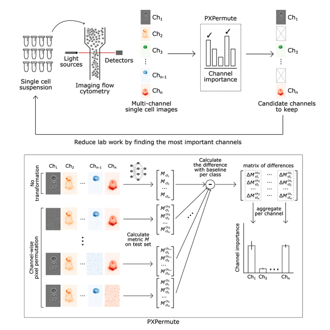
We propose PXPermute as a model-agnostic post hoc method for interpreting channel importance (Figure 1A). In our approach, we work with a dataset of images $x$ with $CH$ channels $x\in X,x:\left\{x^1,...,x^{CH}\right\}$ and their corresponding labels $y$ from $CL$ classes ($y\in Y,Y:\left\{y_1,...,y_{CL}\right\}$). We assume the existence of a supervised multiclass classifier model $f\left(x\right)$ that is trained to predict the label for each image: $f\left(x\right)=\hat{y}$. During the test phase, we apply PXPermute by randomly shuffling pixels in a given channel ($1\le ch\le CH$) of each input image. We evaluate a performance metric $M$ (e.g., accuracy) for each class ($1\le cl\le CL$) based on the classifier’s performance $M_{cl}^{ch,}$. This process is repeated iteratively for each channel of the input image, and we calculate the differences between the original performance $M_{cl}$ (without shuffling any channels) and the new performance $M_{cl}^{ch}$ (${\Delta M}_{cl}^{ch}=M_{cl}-M_{cl}^{ch}$). Finally, the channel importance is determined by aggregating these difference values (e.g., using the median) for each class $\left\{{\Delta M}_1^{ch},{\Delta M}_2^{ch},...,{\Delta M}_{CL}^{ch}\right\}$ across all images (Figure 1B; star methods).

Figure 1.

PXPermute allows identifying the most important fluorescent (FL) channels in a multichannel imaging flow cytometry experiment and thus reduces lab work and expenses

(A) Schematic of a PXPermute embedded end-to-end analysis. In the first part, biologists image thousands of single cells using imaging flow cytometry in different FL and bright-field (BF) channels. The second part, PXPermute, will select the most important channels based on the task.

(B) Schematic of PXPermute, a simple yet powerful method to find the most important channels. In the first step, a performance metric $M_{cl}$ (such as accuracy or F1-score) is calculated per class $cl$. Then, each channel $Ch$ is shuffled, and the performance per class $cl$ is calculated as $M_{cl}^{Ch}$. Finally, the difference between the original performance and the permuted one is calculated. These differences are averaged and yield the channel importance.

We selected three publicly available IFC datasets to demonstrate PXPermute’s potential to rank fluorescent stainings as well as stain-free channels in multichannel images. The first dataset contains 15,311 images of two classes, comprising 8,884 apoptotic cells and 6,427 non-apoptotic cells with only a bright field (BF) and one fluorescent channel (Figure 2A; STAR Methods). The second dataset contains 5,221 images of lymphocytes that form immunological synapses.^23,31 Images contain a single cell, two cells, or more than two cells. They are distributed into the following nine classes: B cells, T cells without signaling, T cells with signaling, T cell with smaller B cells, B and T cells in one layer, synapse without signaling, synapse with signaling, no cell-cell interaction, and multiplets. This dataset includes eight channels: BF, antibody (Ab), CD18, F-actin, major histocompatibility complex (MHC) class II, CD3, P-CD3ζ, and live/dead stainings (Figure 2B; STAR Methods). Considering that the dataset consists of live T or B cells with no Abs, the Ab and live/dead channels do not contain any relevant information. Therefore, they are used as a sanity check in the channel importance analysis. Finally, the white blood cell dataset¹⁸ includes 98,013 images with eight classes and twelve channels. The classes are CD14⁺ monocyte, CD15⁺ neutrophil, CD19⁺ B cell, CD4⁺ T cell, CD56⁺ natural killer (NK), CD8⁺ T cell, NK T cell, and eosinophil. The channels include BF1, CD15, SigL8, CD14, CD19, dark field (DF), CD3, CD45, BF2, CD4, CD56, and CD8 (Figure 2C; STAR Methods).

Figure 2.

Three datasets with various numbers of images and channels are used to evaluate PXPermute

Rows indicate classes, and columns indicate the channels. Channels marked with an asterisk (∗) indicate that those channels have been identified as the most important channels in previous works.

(A) Apoptotic cells: a dataset containing 15,311 images with one stain-free, BF, and an FL channel.

(B) Synapse formation: a dataset containing 5,221 images with one stain-free channel (BF) and seven FL channels, namely antibody (Ab), CD18, F-actin, MHC class II, CD3, P-CD3ζ and live/dead.

(C) White blood cells: a dataset containing 29,994 images with three stain-free channels, two BFs (BF1 and BF2), a dark-field (DF), and nine stained channels including CD15, SigL8, CD14, CD19, CD3, CD45, CD4, CD56, and CD8.

PXPermute detects the most important channels in alignment with biological knowledge

As a proof of concept, we used PXPermute on a ResNet18³² pretrained on ImageNet,³³ a widely used deep learning model for image classification.^34,35 Considering that this model was designed originally for natural images with three channels, we replaced the first layer of the network by matching the number of channels per dataset. Also, the classification layer was changed based on the number of classes in each dataset (see STAR Methods for details). We trained the ResNet18 on each dataset to classify the cells into the given cell types and compared it to the state-of-the-art performance. For the apoptotic vs. non-apoptotic cells, the model reached the performance of F1-macro = 0.97 ± 0.01 (mean and standard deviation from 5-fold cross-validation). The model reached an F1-macro performance of 0.95 ± 0.01 for the synapse formation dataset. Finally, for the white blood cell dataset, our model reached 0.98 ± 0.01 of F1-macro (STAR Methods).

Since no method has been developed for assessing channel importance, we adapted existing pixel-wise interpretation methods, including occlusion,³⁶ DeepLift,³⁷ Guided Grad-CAM,²⁵ integrated gradients,³⁸ and layerwise relevance propagation (LRP)³⁹ (Table 1; STAR Methods). We modified the occlusion method to occlude the images channel-wise to replace the whole channel with 0. Similar to PXPermute, the drop in model performance is considered the channel importance (Figure S1A). The other methods originally provided pixel-wise importance for each image, typically visualized as a heatmap.⁴⁰ We aggregate the pixel importance per channel to adapt them to calculate a channel-wise importance score (Figure S1B). Except for channel-wise occlusion, all these methods are not model agnostic and strongly depend on the quality of the pixel importance estimation and its aggregation to obtain a channel score.

Table 1.

Adaptation of used methods for benchmarking

Method name	Adaptation	Advantages	Disadvantages
PXPermute	none	+ open source + model agnostic + simple concept + keeps the data distribution + no parameter tuning	− higher runtime
Channel-wise occlusion	occluding channels instead of pixels	+ rapid runtime + model agnostic + simple concept + no parameter tuning	− changes the data distribution
Guided GradCAM (Selvaraju et al.25)	using the median of the values per channel	+ rapid runtime + open source	− model specific − requires parameter tuning − needs adaptation
Integrated gradients (Sundararajan et al.38)	using the median of the values per channel	+ rapid runtime + open source	− model specific − requires parameter tuning − needs adaptation
DeepLift (Shrikumar et al.37)	using the median of the values per channel	+ rapid runtime + open source	− model specific − requires parameter tuning − needs adaptation
LRP (Bach et al.39)	using the median of the values per channel	+ rapid runtime + open source	− model-specific − requires parameter tuning − needs adaptation

Apart from PXPermute, designed for channel importance, all other methods were adapted from their original design. Their other advantages and disadvantages are based on model specificity, design complexity, runtime, and the need for tuning.

We benchmarked all interpretation methods on the trained models in the next step. With each model training in the cross-validation scheme, we also run each interpretation method. Therefore, we have five values per method for each channel. To provide a comparative overview, we normalized each channel’s importance to the intervals of 0 and 1 (Figure 3). Hence, the most important channel obtained an importance score of 1, and the least important channel had a score of 0. For simplicity, based on the number of existing channels in the datasets and previous relevant works, we only focus on the top 1 channel for the apoptotic cell dataset and the top 3 channels for the synapse formation and the white blood cell datasets.

Figure 3.

PXPermute robustly identifies the most important channels

Each dataset’s channel importance is normalized between zero and one for PXPermute and five other methods, including channel-wise occlusion, Guided GradCAM, integrated gradients, DeepLift, and layerwise relevance propagation (LRP). The error bars are based on a 5-fold cross-validation scheme, representing the mean with a 95% confidence interval. Channels marked with an asterisk (∗) indicate that those channels have been identified as the most important channels in previous works. Note that PXPermute channel rankings align better with the findings from previous studies than any other method.

We first applied the channel importance methods to the apoptotic cells dataset. Kranich et al. previously showed on this dataset that the fluorescent channel is more important than the BF channel for predicting apoptotic cells.²⁸ PXPermute, channel-wise occlusion, and Guided GradCAM correctly identified the fluorescent channel as the most important channel for predicting apoptotic cells, which aligns with previous work.²⁸ In contrast, integrated gradients, DeepLift, and LRP identify BF as the most important channel (Figures 3A and S2A), leading to a false conclusion on this dataset.

For the synapse formation dataset, we previously showed that the most important channels are CD3, MHC class II, and P-CD3ζ.^23,31 PXPermute identifies the top channels P-CD3ζ, CD3, and MHC class II, in line with previous knowledge (Figures 3B and S2B). Channel-wise occlusion finds the same top 3 channels but in a different order. GradCAM identifies P-CD3ζ, live/dead, and CD18 as the most important channels. This order does not fit our prior knowledge because live/dead is an irrelevant channel, as the original authors only annotated the live cells. Integrated gradients and DeepLift identify CD3, P-CD3ζ, and BF as the most important channels. Finally, LRP identifies CD3, BF, and Ab as the most important channels. This contradicts our knowledge, as no Ab exists in the dataset.

The white blood cell dataset has the largest number of channels and the highest variation of the channel rankings. This dataset had not been used for channel importance before. However, from the work of Lippeveld et al.,¹⁸ it is possible to infer that CD3, CD4, CD56, and CD8 are the most important channels. PXPermute suggests that the top 3 channels are CD56, CD8, and CD4, confirming Lippeveld et al.’s work. Channel-wise occlusion suggests that CD56, CD3, and CD19 are the most important channels. Guided GradCAM suggests that BF1, CD56, and BF2 are the most important channels. Integrated gradients identified CD46, CD19, and BF1 as the most important channels. DeepLift indicates that CD56, CD19, and BF1 are the most important channels. Finally, LRP implies that CD19, BF2, and BF1 are the most important channels (Figures 3C and S2C). Our method-identified channel importance closely aligned with existing baselines and expert findings.^18,23,28

100 repetitions are enough for a stable channel-order identification

We conducted an ablation study using k = 5, 10, 20, 30, 40, 50, 100, 200, 500, and 1,000 to determine the number of repetitions required for PXPermute to yield stable results. Our findings revealed that for apoptotic cells, there was no change in the channel order. However, we observed a change in the channel order for k = 40 and 50 for the synapse formation dataset. Similarly, a difference was noted only for the white blood cell dataset for k = 30. The most significant observation was that the channel order remained unchanged from k = 100 onwards for all datasets. Therefore, we recommend using k = 100 for PXPermute to obtain reliable and robust results.

Identifying and removing unnecessary channels with PXPermute

To validate channel importance rankings suggested by PXPermute and the other methods, we applied the remove-and-retrain principle⁴¹: first, we sorted image channels according to their predicted importance score in ascending order, from the least important channel to the most important. Then, we iteratively removed channels from the dataset, from the least important to the most important channel. Secondly, after each removal, the classification model was retrained on the dataset containing the subset of channels to perform the same classification task as before. During the remove-and-retrain process, we fixed model hyperparameters. We repeated this procedure for every channel ranking (see Figure 3). In an ideal scenario, removing a channel that is not important for the model prediction should not affect model performance. Removing a channel that is important for the model should highly affect its performance. Therefore, if the performance of a model during the remove-and-retrain process drops faster for a given sequence of channels than for another sequence of channels, then it shows that the sequence ordering was not optimal. To numerically compare the drops in classification performance, we calculate the average F1-macro across all the runs (see Figure 3).

For the apoptotic cell dataset, the order suggested by PXPermute, channel-wise occlusion, and Guided GradCAM was the optimal sequence. They showed the highest performance (average F1-macro of 0.97 ± 0.01, n = 10 based on 5-fold cross-validation and two channels). They were followed by LRP (0.83 ± 0.14), integrated gradients (0.83 ± 0.15), and DeepLift (0.82 ± 0.15) (Figure 4A; Table S1).

Figure 4.

PXPermute outperforms other methods in identifying the correct channel ranking based on a remove-and-retrain procedure

The remove-and-retrain based on the channel ranking is performed on the apoptotic cell (2 channels), synapse formation (8 channels), and white blood cell (12 channels) datasets. The error bars represent the mean with a 95% confidence interval. In each case, the channels are sorted in ascending order according to their predicted importance score, from the least important channel to the most important. Then, the channels are iteratively removed from the dataset, from the least important to the most important channel. After each removal, the classification model was retrained on the dataset containing the subset of channels to perform the same classification task as before. Methods with better rankings would stay higher throughout the plot. PXPermute performed better than other methods in finding the optimal channel rankings.

For the synapse formation dataset, PXPermute predicted the best sequence of channels (average F1-macro = 0.92 ± 0.04, n = 40 based on 5-fold cross-validation and eight channels). It was followed by Guided GradCAM (0.90 ± 0.05), DeepLift (0.89 ± 0.07), channel-wise occlusion (0.89 ± 0.08), integrated gradients (0.88 ± 0.07), and LRP (0.86 ± 0.08) (Figure 4B; Table S1).

For the white blood cell dataset, PXPermute, channel-wise occlusion, and DeepLift predicted the best sequence of channels (average F1-macro = 0.97 ± 0.02, n = 60 based on 5-fold cross-validation and 12 channels). It was followed by integrated gradients (0.96 ± 0.02), Guided GradCAM (0.94 ± 0.06), and LRP (0.90 ± 0.05) (Figure 4C; Table S1). The same pattern could be observed for average F1-micro and accuracy. Therefore, PXPermute is the only method that correctly detects the order of the importance of the channels in all datasets (Figure 4).

PXPermute finds the optimal panel with a minimal number of stainings

Identifying a minimal set of stainings required for a downstream task has manifold advantages, such as the potential to reduce staining artifacts and save cost and time in sample preparation. It also allows adding new, more meaningful stainings to the panel. Therefore, identifying the minimum set of channels a model requires to deliver optimal performance is highly beneficial. To investigate this effect, we compared the model’s performance in three scenarios: (1) the model was trained with only non-stained channels (no florescent channels), (2) it was trained with only the most important channels according to PXPermute plus the non-stain channels (minimal number of florescent channels), and (3) it was trained with all the fluorescent and non-stain channels. We conducted these experiments on the synapse formation and the white blood cell dataset (Figure 5) and skipped the apoptotic cell dataset, as it has only two channels.

Figure 5.

PXPermute finds an optimal channel selection that performs similarly to using all the channels

For the synapse formation (A) and white blood cell (B) datasets, the model was trained on the stain-free channels (lower bound), stain-free + top 3 channels identified by PXPermute, and all channels (upper bound). The error bars represent the mean with a 95% confidence interval. PXPermute rankings lead to fewer stainings (3 out of 7 in A, 3 out of 8 in B) without a significant loss in performance.

For the synapse formation, the stain-free selection of channels (BF) achieves 0.78 ± 0.09 F1-macro in a 5-fold cross-validation setup. Adding the suggested channels from PXPermute, namely, MHC class II, CD3, and P-CD3ζ, improves the classification to 0.93 ± 0.01 F1-macro, which is not so different from 0.94 ± 0.01 F1-macro, which is the accuracy when using all channels. For the white blood cell dataset, the stain-free selection of channels (BF1, BF2, and DF) achieves 0.84 ± 0.04 F1-macro. By adding only the three most important channels identified by PXPermute, namely CD4, CD56, and CD8, the classifier archives the performance of 0.97 ± 0.01 F1-macro, which is not significantly less than a model trained on all channels, reaching 0.97 ± 0.00 F1-macro. We have shown that PXPermute can identify the most important channels for a cell classification task. The required channels can be halved without significantly decreasing the model’s performance.

Discussion

In this study, we introduced PXPermute, a post-model interpretability method that assesses the impact of fluorescent stainings on cell classification. By applying PXPermute to three publicly available IFC datasets, we demonstrated its efficacy in accurately identifying the most significant channels in accordance with biological principles. Moreover, PXPermute can facilitate panel optimization by recommending fewer stainings that maintain comparable performance to using all channels.

While multicolor fluorescent staining panel optimization for flow and mass cytometry is a well-established research field,¹⁰ there is little systematic analysis and methodology for IFC, with only a handful of works touching upon its significance. These works either use a feature importance from an explainable classifier such as random forest^27,28 or a greedy search by trying combinations of channels to find the most important channels.^23,26 Although these methods can be powerful tools, the former prohibits using deep learning algorithms, and the latter can be exhaustive and computationally costly. PXPermute addresses these limitations and provides a model-agnostic interpretability method for feature ranking that can be applied independently of the number of channels or model architecture. Additionally, our research represents one of the first comprehensive investigations into systematically exploring channel and staining importance for imaging data.

To demonstrate PXPermute’s robustness, we applied it to three different publicly available datasets. We identified that the fluorescent channel is more important than the BF channel for the apoptotic vs. non-apoptotic cells, which aligns with the previous work.²⁸ MHC class II, CD3, and P-CD3ζ were identified in the synapse formation study to detect immunological synapses, again in alignment with the original study.²³ While other methods also found a high-performing combination of channels, none aligned with underlying biology, and they were probably only hinting at possible artifacts in the dataset. Finally, the authors did not provide a clear channel importance ranking for the white blood cell dataset.¹⁸ However, it was possible to infer from their work that adding CD4, CD56, and CD8 can improve the classification performance significantly. This is the same combination as suggested by PXPermute. An essential point to consider is that these fluorescent channels are shown to be important for their respective downstream task, and their importance can change for a different task. Finally, apart from the current datasets, PXPermute can potentially be used on other data modalities, such as multiplex IF images^42,43,44 and multiplexed protein maps,^45,46 where the data include multiple fluorescent stainings with complex morphologies.

To effectively utilize PXPermute in laboratory conditions, we recommend performing a small experiment with all possible stainings and applying PXPermute to the data. After the post hoc analysis, the main experiment can be conducted using the selected channels. For example, let us assume the objective of optimizing the panel for a particular use case with 20 candidate markers. Considering that a machine like Amnis can capture ten fluorescent channels at a time, the experimental approach can be divided into three stages: in the first stage, an initial set of ten markers is examined, followed by an assessment of the remaining ten markers in the second stage. Upon completion of these preliminary runs, the top 5 markers in each experiment are identified. In the final stage, the experiment is conducted with the union of those top 5 markers, selected based on the results from the initial two stages (2 × 5 = 10). Again, PXPermute can be applied to find the best combination of markers.

A potential limitation in this work is the need to repeat the execution of PXPermute multiple times to enhance its robustness. This iterative process can be time consuming depending on the dataset size and the number of channels involved. Nonetheless, PXPermute is still faster than the leave-one-channel-out strategy. PXPermute takes 65 ± 10 min with 5-fold cross-validation for the white blood cell dataset with 12 channels on a machine with a GPU and 16 CPUs. We observed that training a ResNet18 model on the same data and hardware takes 28 ± 1 min. For the leave-one-channel-out strategy, one must train 13 independent models, which takes approximately 13 × 28 = 364 min, more than five times more than PXPermute. In the case of finding the best combination of channels, one needs to train 2¹² − 1 = 4,095 different models, which is highly exhaustive. Furthermore, it is worth noting that PXPermute has been designed to support parallelization, enabling significant acceleration of the calculations and mitigating this limitation. Another limitation is that PXPermute is designed for a supervised learning setup where experts must annotate the images. This process of annotation can be time consuming and, hence, challenging. Therefore, finding an unsupervised method for evaluating fluorescent stainings can be an attractive area for research.

In summary, PXPermute is the first method that systematically studies channel importance for deep learning models and can potentially lead to optimizing the workflow of biologists in the lab. PXPermute can be implemented for panel optimization and can benefit biologists in their lab work.

Limitations of the study

Notably, PXPermute must be executed multiple times to obtain robust results. This can be time consuming, especially with many channels. However, our approach is still faster than the baseline leave-one-channel-out strategy (see discussion). A general limitation is that PXPermute is designed for supervised learning scenarios and relies on annotated data. This limits the application of PXPermute for scenarios where sufficient high-quality annotations are available.

STAR★Methods

Key resources table

REAGENT or RESOURCE	SOURCE	IDENTIFIER
Deposited data
Apoptotic cells dataset	Kranich et al.28	https://doi.org/10.1080/20013078.2020.1792683
Synapse formation dataset	Essig et al.23,31	https://doi.org/10.5061/dryad.ht76hdrk7
White blood cell dataset	Lippeveld et al.18	https://doi.org/10.1002/cyto.a.23920
Software and algorithms
PXPermute	Current work	https://doi.org/10.5281/zenodo.10495259 https://github.com/marrlab/pxpermute
scifAI	Shetab Boushehri et al.23,31	https://github.com/marrlab/scifAI

Resource availability

Lead contact

Further information and requests for resources and reagents should be directed to and will be fulfilled by the lead contact, Carsten Marr (carsten.marr@helmholtz-munich.de).

Materials availability

This study did not generate or use any biological samples or generate new unique reagents.

Data and code availability

• •All datasets in this study are from public data. All the links and required information are provided in the Methods section. Additionally, the DOIs are listed in the key resources table.
• •The code and instructional notebooks on running the code and building analysis pipelines are here: https://github.com/marrlab/pxpermute with the DOI: https://doi.org/10.5281/zenodo.10495259
• •Any additional information required to reanalyze the data reported in this paper is available from the lead contact upon request.

Method details

Datasets

All data studied in this work was acquired through imaging flow cytometry. For model training and testing, brightfield and fluorescent channels were used. In the datasets with a strong imbalance, the training set was oversampled by randomly selecting indices from minority classes with replacement. All images were rescaled to 0 and 1 using the minimum and maximum of the datasets.

Apoptotic cells dataset -

This dataset was published by Kranich et al.,²⁸ who not only solved the binary classification task (apoptotic vs. non-apoptotic cell) but also studied the channel importance directly. Each class is represented by only two channels, one fluorescent (Figure 2A). The images were cropped to 32x32. The dataset was accessed here: https://github.com/theislab/dali/tree/master/data.

Synapse formation dataset -

Shetab Boushehri and Essig et al. published this dataset^23,31 to study the process of synapse formation using IFC. Their dataset includes nearly 2,8 million images containing T cells and B-LCL cells or their conjugates; only 5,221 are labeled by an expert. Each image contains eight channels containing brightfield (BF, stain-free), antibody (Ab, fluorescent), CD18 (fluorescent), F-actin (fluorescent), MHCII (fluorescent), CD3 (fluorescent), P-CD3ζ (fluorescent), and Live/Dead (fluorescent) (Figure 2B). This annotated subset only contains images of live cells with no antibodies. Therefore, Ab and Live/Dead channels are redundant. Moreover, they showed that for the classification of synapses, the most important channels are MHCII, CD3, and P-CD3ζ. Since the images are in different sizes, they have been padded to 128x128 to prepare them for training. The dataset was accessed here: https://doi.org/10.5061/dryad.ht76hdrk7.

White blood cell dataset -

The white blood cell dataset¹⁸ (WBC) contains 98,013 IFC images, each with twelve channels, which were obtained from two whole blood samples of patients. In each image, a single cell is contained, with eight classes (Figure 2C): natural killer (NK) cells (669 samples), neutrophils (18,325 samples), eosinophils (1,537 samples), monocytes (1,282 samples), B cells (889 samples), T cells CD8⁺ (1,788 samples) and CD4⁺ (4,476 samples), natural killer T (NKT) cells (1,028 samples), and a separate class comprising unidentifiable cells (1,286 samples). All images were reshaped to 64x64. The channels comprise two brightfield channels, one dark field channel, and nine stained channels. Lippeveld et al.¹⁸ have shown that stain-free data suffices to classify monocytes and neutrophils, but to classify others reliably, the dataset must include stained channels. The dataset was accessed here: https://cloud.irc.ugent.be/public/index.php/s/assnP3Z2FjTbztc.

Classification models

In this work, we analyzed a commonly used deep learning classifier. The models' decision-making process cannot be interpreted without applying explainability methods. We selected ResNet18 (16) from all image classification models due to its good performance reported in the previous works.^18,23,34 We used weights pre-trained on ImageNet³³ implemented in the PyTorch package.⁴⁷ To utilize the scikit-learn⁴⁸ pipeline for the deep learning model, we used the model wrapper from the Skorch library.⁴⁹ The pipeline comprises the data transformation step, which includes normalizing samples with the 1st and 99th percentile of images for each dataset, random vertical and horizontal flips, and random noise. To evaluate and compare model accuracy, we have used the F1-score. The model was trained with the cross-entropy loss and AdamW optimizer, with a batch size of 128. The learning rate was set to 0.001 when initializing a new model before starting the training and was kept decreasing by a factor of 0.5 if there was no improvement in the F1-macro score of the validation set for five epochs straight. We have also applied the early stopping technique, abrupting the training if the same metric stays constant ±0.0001 for 50 epochs.

Model interpretation

To the best of the authors’ knowledge, no methods can be directly applied to the pre-trained model to evaluate the channel importance. However, some methods evaluate the importance of a single or set of pixels. Thus, our first approach was to aggregate their results per channel. The aggregation method takes the median of the pixel values per channel.

In this study, we have used the following pixel-wise interpretation methods to analyze the channel importance.

PxPermutes -

Analog to pixel-wise interpretation, channel importance can be estimated via conducting sensitive analysis: measuring changes in the model output caused by changes in input. However, our method permutes pixels in the channel compared to occlusion,³⁶ which replaces a specific pixel area with an occluding mask. We avoid violating the critical principle of machine learning, which states that training and test sets must be drawn from the same distribution.

Permuting pixels per channel destroys the structural information contained in contours, edges, or areas. It can still be guaranteed that the degradation in the model performance was not due to the artifacts in the pixel intensity distribution.

PXPermute augments each image channel in a dataset by permuting the pixels of each channel $k$ times. For a dataset with $N$ images, PXPermute generates $N\ast k$ modified multichannel images; see Figure 1B. The user can define the parameter $k$: a larger $k$ leads to more robust results but requires more computational resources. For a very large $k$, the algorithm’s complexity increases and approaches the brute force search approach, in which the model is retrained and re-evaluated for all possible channel combinations. We test PXPermute on a single-cell classification task, measuring the drop in the F1-score as our metric for performance evaluation. PXPermute design is inspired by the previous works on feature importance as well as interpretability of CNN models,^36,50,51 which tries to solve the disadvantages of the other interpretability methods and combine all the strengths, such as independence on the model architecture, preserving the same train/test pixel intensity distribution, and simplicity in one method.

Occlusion

Zeiler et al.³⁶ introduced the idea of estimating the importance of the part of the scene by replacing it with a gray square and observing the classifier’s output. Such a technique was called sensitive analysis or occlusion sensitivity. Later, Zintgraf et al. initiated removing the information from an image completely and calculating the effect. In addition, the authors proposed optimizing the occluding strategy by introducing the marginalization of the occluded pixel. Finally, the method was studied further and formalized by Samek et al.⁵²: $R_i=f\left(x\right)-f\left(x⨀\left(1-m_i\right)\right)$, where $R$ is a heatmap, $f$ is a classifier function, $m$ is an indicator function for removing the patch or feature, and $⨀$ denotes the element-wise product. As a result, the heatmap highlights the patches (pixels) stronger if their removal affected the classifier results more. Due to its mechanism, the method is referred to as the perturbation-based forward propagation method.

Despite the simplicity of the concept, the method has its disadvantages. One of them is computational complexity. Every time one pixel or patch is occluded, the output must be recomputed. The computational time can rapidly become infeasible if the input is huge. Another problem of the approach is the saturation effect. It occurs when removing only one patch at a time does not affect the output, but removing multiple patches simultaneously does. This leads to misinterpretation and wrong conclusions. In addition, occluding the test image changes its pixel intensity distribution, which can lead to a corrupted interpretation.

Guided Grad-CAM

another way of interpreting a model is backpropagating an important signal from the output toward the input. If occlusion requires perturbing and passing the input forward multiple times, this approach needs to do a backward pass only once, making it computationally efficient. Nevertheless, gradient-based backpropagation methods have drawbacks, including the saturation effect and being designed for convolutional neural networks only.

Guided Grad-CAM is an element-wise product of the results of two other interpretational approaches: Guided Backpropagation and Grad-CAM.²⁵ On the one hand, Grad-CAM uses the last convolutional layer’s gradient information to evaluate each neuron’s importance for a specific class. On the other hand, Guided Backpropagation isn’t class-discriminative but rather highlights details of an image by visualizing gradients in high resolution. Thus, fusing both methods results in high-resolution class-discriminative saliency maps.

DeepLift

with this method, authors addressed the saturation problem by considering gradient-based interpretation approaches.³⁷ Instead of propagating the gradients, this approach suggests propagating the difference from a reference. For example, the reference input can be blurred images or images containing only the background color. Consequently, the method’s output strongly depends on the definition of reference input, which requires data or domain knowledge.

Layer-wise relevance propagation (LRP) -

the idea is to calculate the relevance of input features to the particular prediction.³⁹ The relevance is propagated from the output back to the input layers by distributing the output value into relevance scores for each underlying neuron sequentially based on the model’s weights and activations. So that the neuron with a positive contribution receives a proportionally bigger relevance score. The method applies the set of propagation rules depending on the activations and layers, making this method more difficult to implement and more computationally expensive if applied to a large-scale model.

Quantification and statistical analysis

Quantification and statistical analysis can be found in the text and figure legends. All necessary information, including the number of samples and the quantity measured, is reported in the corresponding section in the text or figure legend.

Published: February 26, 2024

References

- 1.Rane A.S., Rutkauskaite J., deMello A., Stavrakis S. High-Throughput Multi-parametric Imaging Flow Cytometry. Chem. 2017;3:588–602. doi: 10.1016/j.chempr.2017.08.005. [DOI] [Google Scholar]
- 2.Barteneva N.S., Vorobjev I.A. Imaging flow cytometry. J. Immunol. Methods. 2016 doi: 10.1007/978-1-4939-3302-0_1. [DOI] [PubMed] [Google Scholar]
- 3.Doan M., Vorobjev I., Rees P., Filby A., Wolkenhauer O., Goldfeld A.E., Lieberman J., Barteneva N., Carpenter A.E., Hennig H. Diagnostic Potential of Imaging Flow Cytometry. Trends Biotechnol. 2018;36:649–652. doi: 10.1016/j.tibtech.2017.12.008. [DOI] [PubMed] [Google Scholar]
- 4.Barteneva N.S., Fasler-Kan E., Vorobjev I.A. Imaging Flow Cytometry: Coping with Heterogeneity in Biological Systems. J. Histochem. Cytochem. 2012;60:723–733. doi: 10.1369/0022155412453052. [DOI] [PMC free article] [PubMed] [Google Scholar]
- 5.Blasi T., Hennig H., Summers H.D., Theis F.J., Cerveira J., Patterson J.O., Davies D., Filby A., Carpenter A.E., Rees P. Label-free cell cycle analysis for high-throughput imaging flow cytometry. Nat. Commun. 2016;7 doi: 10.1038/ncomms10256. [DOI] [PMC free article] [PubMed] [Google Scholar]
- 6.Eulenberg P., Köhler N., Blasi T., Filby A., Carpenter A.E., Rees P., Theis F.J., Wolf F.A. Reconstructing cell cycle and disease progression using deep learning. Nat. Commun. 2017;8:463. doi: 10.1038/s41467-017-00623-3. [DOI] [PMC free article] [PubMed] [Google Scholar]
- 7.Chlis N.-K., Rausch L., Brocker T., Kranich J., Theis F.J. Predicting single-cell gene expression profiles of imaging flow cytometry data with machine learning. Nucleic Acids Res. 2020;48:11335–11346. doi: 10.1093/nar/gkaa926. [DOI] [PMC free article] [PubMed] [Google Scholar]
- 8.Lee K.C.M., Wang M., Cheah K.S.E., Chan G.C.F., So H.K.H., Wong K.K.Y., Tsia K.K. Quantitative Phase Imaging Flow Cytometry for Ultra-Large-Scale Single-Cell Biophysical Phenotyping. Cytometry A. 2019;95:510–520. doi: 10.1002/cyto.a.23765. [DOI] [PubMed] [Google Scholar]
- 9.McLaughlin B.E., Baumgarth N., Bigos M., Roederer M., De Rosa S.C., Altman J.D., Nixon D.F., Ottinger J., Oxford C., Evans T.G., Asmuth D.M. Nine-color flow cytometry for accurate measurement of T cell subsets and cytokine responses. Part I: Panel design by an empiric approach. Cytometry A. 2008;73:400–410. doi: 10.1002/cyto.a.20555. [DOI] [PMC free article] [PubMed] [Google Scholar]
- 10.Mahnke Y., Chattopadhyay P., Roederer M. Publication of optimized multicolor immunofluorescence panels. Cytometry A. 2010;77:814–818. doi: 10.1002/cyto.a.20916. [DOI] [PubMed] [Google Scholar]
- 11.Roos E.O., Bonnet-Di Placido M., Mwangi W.N., Moffat K., Fry L.M., Waters R., Hammond J.A. OMIP-085: Cattle B-cell phenotyping by an 8-color panel. Cytometry A. 2023;103:12–15. doi: 10.1002/cyto.a.24683. [DOI] [PMC free article] [PubMed] [Google Scholar]
- 12.Mincham K.T., Snelgrove R.J. OMIP-086: Full spectrum flow cytometry for high-dimensional immunophenotyping of mouse innate lymphoid cells. Cytometry A. 2023;103:110–116. doi: 10.1002/cyto.a.24702. [DOI] [PMC free article] [PubMed] [Google Scholar]
- 13.Doyle C.M., Fewings N.L., Ctercteko G., Byrne S.N., Harman A.N., Bertram K.M. OMIP 082: A 25-color phenotyping to define human innate lymphoid cells, natural killer cells, mucosal-associated invariant T cells, and γδ T cells from freshly isolated human intestinal tissue. Cytometry A. 2022;101:196–202. doi: 10.1002/cyto.a.24529. [DOI] [PubMed] [Google Scholar]
- 14.Sponaugle A., Abad-Fernandez M., Goonetilleke N. OMIP-087: Thirty-two parameter mass cytometry panel to assess human CD4 and CD8 T cell activation, memory subsets, and helper subsets. Cytometry A. 2023;103:184–188. doi: 10.1002/cyto.a.24707. [DOI] [PMC free article] [PubMed] [Google Scholar]
- 15.Birrer F., Brodie T., Stroka D. OMIP-088: Twenty-target imaging mass cytometry panel for major cell populations in mouse formalin fixed paraffin embedded liver. Cytometry A. 2023;103:189–192. doi: 10.1002/cyto.a.24714. [DOI] [PubMed] [Google Scholar]
- 16.Barros-Martins J., Bruni E., Fichtner A.S., Cornberg M., Prinz I. OMIP-084: 28-color full spectrum flow cytometry panel for the comprehensive analysis of human γδ T cells. Cytometry A. 2022;101:856–861. doi: 10.1002/cyto.a.24564. [DOI] [PubMed] [Google Scholar]
- 17.Hennig H., Rees P., Blasi T., Kamentsky L., Hung J., Dao D., Carpenter A.E., Filby A. An open-source solution for advanced imaging flow cytometry data analysis using machine learning. Methods. 2017;112:201–210. doi: 10.1016/j.ymeth.2016.08.018. [DOI] [PMC free article] [PubMed] [Google Scholar]
- 18.Lippeveld M., Knill C., Ladlow E., Fuller A., Michaelis L.J., Saeys Y., Filby A., Peralta D. Classification of Human White Blood Cells Using Machine Learning for Stain-Free Imaging Flow Cytometry. Cytometry A. 2020;97:308–319. doi: 10.1002/cyto.a.23920. [DOI] [PubMed] [Google Scholar]
- 19.Ota S., Sato I., Horisaki R. Implementing machine learning methods for imaging flow cytometry. Microscopy. 2020;69:61–68. doi: 10.1093/jmicro/dfaa005. [DOI] [PubMed] [Google Scholar]
- 20.Luo S., Shi Y., Chin L.K., Hutchinson P.E., Zhang Y., Chierchia G., Talbot H., Jiang X., Bourouina T., Liu A.-Q. Machine-learning-assisted intelligent imaging flow cytometry: A review. Adv. Intell. Syst. 2021;3 doi: 10.1002/aisy.202100073. [DOI] [Google Scholar]
- 21.Lippeveld M., Peralta D., Filby A., Saeys Y. A scalable, reproducible and open-source pipeline for morphologically profiling image cytometry data. bioRxiv. 2022 doi: 10.1101/2022.10.24.512549. Preprint at. [DOI] [PubMed] [Google Scholar]
- 22.Timonen V.A., Kerkelä E., Impola U., Penna L., Partanen J., Kilpivaara O., Arvas M., Pitkänen E. DeepIFC: virtual fluorescent labeling of blood cells in imaging flow cytometry data with deep learning. bioRxiv. 2022 doi: 10.1101/2022.08.10.503433. Preprint at. [DOI] [PubMed] [Google Scholar]
- 23.Shetab Boushehri S., Essig K., Chlis N.-K., Herter S., Bacac M., Theis F.J., Glasmacher E., Marr C., Schmich F. Explainable machine learning for profiling the immunological synapse and functional characterization of therapeutic antibodies. Nat. Commun. 2023;14:7888. doi: 10.1038/s41467-023-43429-2. [DOI] [PMC free article] [PubMed] [Google Scholar]
- 24.Strobl C., Boulesteix A.-L., Kneib T., Augustin T., Zeileis A. Conditional variable importance for random forests. BMC Bioinf. 2008;9:307. doi: 10.1186/1471-2105-9-307. [DOI] [PMC free article] [PubMed] [Google Scholar]
- 25.Selvaraju R.R., Cogswell M., Das A., Vedantam R., Parikh D., Batra D. 2017 IEEE International Conference on Computer Vision. ICCV); 2017. Grad-CAM: Visual Explanations from Deep Networks via Gradient-Based Localization; pp. 618–626. [DOI] [Google Scholar]
- 26.Doan M., Case M., Masic D., Hennig H., McQuin C., Caicedo J., Singh S., Goodman A., Wolkenhauer O., Summers H.D., et al. Label-Free Leukemia Monitoring by Computer Vision. Cytometry A. 2020;97:407–414. doi: 10.1002/cyto.a.23987. [DOI] [PMC free article] [PubMed] [Google Scholar]
- 27.Nassar M., Doan M., Filby A., Wolkenhauer O., Fogg D.K., Piasecka J., Thornton C.A., Carpenter A.E., Summers H.D., Rees P., Hennig H. Label-Free Identification of White Blood Cells Using Machine Learning. Cytometry A. 2019;95:836–842. doi: 10.1002/cyto.a.23794. [DOI] [PMC free article] [PubMed] [Google Scholar]
- 28.Kranich J., Chlis N.-K., Rausch L., Latha A., Schifferer M., Kurz T., Foltyn-Arfa Kia A., Simons M., Theis F.J., Brocker T. In vivo identification of apoptotic and extracellular vesicle-bound live cells using image-based deep learning. J. Extracell. Vesicles. 2020;9 doi: 10.1080/20013078.2020.1792683. [DOI] [PMC free article] [PubMed] [Google Scholar]
- 29.Comeau J.W.D., Costantino S., Wiseman P.W. A guide to accurate fluorescence microscopy colocalization measurements. Biophys. J. 2006;91:4611–4622. doi: 10.1529/biophysj.106.089441. [DOI] [PMC free article] [PubMed] [Google Scholar]
- 30.Aaron J.S., Taylor A.B., Chew T.-L. Image co-localization - co-occurrence versus correlation. J. Cell Sci. 2018;131 doi: 10.1242/jcs.211847. [DOI] [PubMed] [Google Scholar]
- 31.Essig K., Boushehri S.S., Marr C., Schmich F., Glasmacher E. 2022. An Imaging Flow Cytometry Dataset for Profiling the Immunological Synapse of Therapeutic Antibodies. [DOI] [Google Scholar]
- 32.He K., Zhang X., Ren S., Sun J. 2016 IEEE Conference on Computer Vision and Pattern Recognition (CVPR) 2016. Deep Residual Learning for Image Recognition; pp. 770–778. [DOI] [Google Scholar]
- 33.Deng J., Dong W., Socher R., Li L.-J., Li K., Fei-Fei L. 2009 IEEE Conference on Computer Vision and Pattern Recognition. 2009. ImageNet: A large-scale hierarchical image database; pp. 248–255. [DOI] [Google Scholar]
- 34.Shetab Boushehri S., Qasim A.B., Waibel D., Schmich F., Marr C. Artificial Neural Networks and Machine Learning – ICANN 2022. Springer International Publishing; 2022. Systematic Comparison of Incomplete-Supervision Approaches for Biomedical Image Classification; pp. 355–365. [DOI] [Google Scholar]
- 35.Xie Y., Richmond D. Computer Vision – ECCV 2018 Workshops. Springer International Publishing; 2019. Pre-training on Grayscale ImageNet Improves Medical Image Classification; pp. 476–484. [DOI] [Google Scholar]
- 36.Zeiler M.D., Fergus R. Computer Vision – ECCV 2014. Springer International Publishing; 2014. Visualizing and Understanding Convolutional Networks; pp. 818–833. [DOI] [Google Scholar]
- 37.Shrikumar, A., Greenside, P., and Kundaje, A. (06--11 Aug 2017). Learning Important Features Through Propagating Activation Differences. In Proceedings of the 34th International Conference on Machine Learning Proceedings of Machine Learning Research., D. Precup and Y. W. Teh, eds. (PMLR), pp. 3145–3153
- 38.Sundararajan, M., Taly, A., and Yan, Q. (06--11 Aug 2017). Axiomatic Attribution for Deep Networks. In Proceedings of the 34th International Conference on Machine Learning Proceedings of Machine Learning Research., D. Precup and Y. W. Teh, eds. (PMLR), pp. 3319–3328
- 39.Bach S., Binder A., Montavon G., Klauschen F., Müller K.R., Samek W. On Pixel-Wise Explanations for Non-Linear Classifier Decisions by Layer-Wise Relevance Propagation. PLoS One. 2015;10 doi: 10.1371/journal.pone.0130140. [DOI] [PMC free article] [PubMed] [Google Scholar]
- 40.Teng Q., Liu Z., Song Y., Han K., Lu Y. A survey on the interpretability of deep learning in medical diagnosis. Multimed. Syst. 2022;28:2335–2355. doi: 10.1007/s00530-022-00960-4. [DOI] [PMC free article] [PubMed] [Google Scholar]
- 41.Hooker S., Erhan D., Kindermans P.-J., Kim B. A benchmark for interpretability methods in deep neural networks. arXiv. 2018 doi: 10.48550/arXiv.1806.10758. Preprint at. [DOI] [Google Scholar]
- 42.Eng J., Bucher E., Hu Z., Zheng T., Gibbs S.L., Chin K., Gray J.W. A framework for multiplex imaging optimization and reproducible analysis. Commun. Biol. 2022;5:438. doi: 10.1038/s42003-022-03368-y. [DOI] [PMC free article] [PubMed] [Google Scholar]
- 43.Lin J.-R., Izar B., Wang S., Yapp C., Mei S., Shah P.M., Santagata S., Sorger P.K. Highly multiplexed immunofluorescence imaging of human tissues and tumors using t-CyCIF and conventional optical microscopes. Elife. 2018;7 doi: 10.7554/eLife.31657. [DOI] [PMC free article] [PubMed] [Google Scholar]
- 44.Rojas F., Hernandez S., Lazcano R., Laberiano-Fernandez C., Parra E.R. Multiplex Immunofluorescence and the Digital Image Analysis Workflow for Evaluation of the Tumor Immune Environment in Translational Research. Front. Oncol. 2022;12 doi: 10.3389/fonc.2022.889886. [DOI] [PMC free article] [PubMed] [Google Scholar]
- 45.Spitzer H., Berry S., Donoghoe M., Pelkmans L., Theis F.J. Learning consistent subcellular landmarks to quantify changes in multiplexed protein maps. bioRxiv. 2022 doi: 10.1101/2022.05.07.490900. Preprint at. [DOI] [PMC free article] [PubMed] [Google Scholar]
- 46.Gut G., Herrmann M.D., Pelkmans L. Multiplexed protein maps link subcellular organization to cellular states. Science. 2018;361 doi: 10.1126/science.aar7042. [DOI] [PubMed] [Google Scholar]
- 47.Paszke A., Gross S., Massa F., Lerer A., Bradbury J., Chanan G., Killeen T., Lin Z., Gimelshein N., Antiga L., et al. PyTorch: An imperative style, high-performance deep learning library. arXiv. 2019 doi: 10.48550/arXiv.1912.01703. Preprint at. [DOI] [Google Scholar]
- 48.Pedregosa F., Varoquaux G., Gramfort A., Michel V., Thirion B., Grisel O., Blondel M., Müller A., Nothman J., Louppe G., et al. Scikit-learn: Machine Learning in Python. arXiv. 2012:2825–2830. doi: 10.48550/arXiv.1201.0490. Preprint at. [DOI] [Google Scholar]
- 49.Skorch Documentation — Skorch 0.12.1 Documentation https://skorch.readthedocs.io/en/stable/
- 50.Altmann A., Toloşi L., Sander O., Lengauer T. Permutation importance: a corrected feature importance measure. Bioinformatics. 2010;26:1340–1347. doi: 10.1093/bioinformatics/btq134. [DOI] [PubMed] [Google Scholar]
- 51.Breiman L. Random Forests. Mach. Learn. 2001;45:5–32. doi: 10.1023/A:1010933404324. [DOI] [Google Scholar]
- 52.Samek W., Binder A., Montavon G., Lapuschkin S., Muller K.-R. Evaluating the Visualization of What a Deep Neural Network Has Learned. IEEE Trans. Neural Netw. Learn. Syst. 2017;28:2660–2673. doi: 10.1109/TNNLS.2016.2599820. [DOI] [PubMed] [Google Scholar]
Associated Data
This section collects any data citations, data availability statements, or supplementary materials included in this article.
Supplementary Materials
Data Availability Statement