

Abstract
Background and Aims
Contrasting patterns of host and microbiome biogeography can provide insight into the drivers of microbial community assembly. Distance–decay relationships are a classic biogeographical pattern shaped by interactions between selective and non-selective processes. Joint biogeography of microbiomes and their hosts is of increasing interest owing to the potential for microbiome-facilitated adaptation.
Methods
In this study, we examine the coupled biogeography of the model macroalga Durvillaea and its microbiome using a combination of genotyping by sequencing (host) and 16S rRNA amplicon sequencing (microbiome). Alongside these approaches, we use environmental data to characterize the relationship between the microbiome, the host, and the environment.
Key Results
We show that although the host and microbiome exhibit shared biogeographical structure, these arise from different processes, with host biogeography showing classic signs of geographical distance decay, but with the microbiome showing environmental distance decay. Examination of microbial subcommunities, defined by abundance, revealed that the abundance of microbes is linked to environmental selection. As microbes become less common, the dominant ecological processes shift away from selective processes and towards neutral processes. Contrary to expectations, we found that ecological drift does not promote structuring of the microbiome.
Conclusions
Our results suggest that although host macroalgae exhibit a relatively ‘typical’ biogeographical pattern of declining similarity with increasing geographical distance, the microbiome is more variable and is shaped primarily by environmental conditions. Our findings suggest that the Baas Becking hypothesis of ‘everything is everywhere, the environment selects’ might be a useful hypothesis to understand the biogeography of macroalgal microbiomes. As environmental conditions change in response to anthropogenic influences, the processes structuring the microbiome of macroalgae might shift, whereas those governing the host biogeography are less likely to change. As a result, increasingly decoupled host–microbe biogeography might be observed in response to such human influences.
Keywords: Durvillaea, microbiome, holobiont, biogeography, distance decay, macroalgae
INTRODUCTION
Biogeographical patterns of host-associated microbial communities vary considerably, and understanding the drivers of these patterns is a crucial aspect of microbial ecology (Graco-Roza et al., 2022; Härer and Rennison, 2023). For example, shared biogeographical patterns of a host and its microbiome, or lack thereof, can provide crucial insight into biogeographical structure and the role of hosts as vectors for microbial dispersal (Tesson et al., 2015; Mony et al., 2022). Flamingos show a high degree of localized microbiome structure despite genetic panmixia of the host population (Gillingham et al., 2019), and the macroalga Phyllospora shares biogeographical structure with its microbiome (Wood et al., 2022). Conversely, microbiome structure of the macroalga Ecklonia radiata is shaped more by host conditions than geography (Marzinelli et al., 2015). Differing patterns of host–microbiome relationships can also indicate the relative importance of niche and neutral processes, although being associated with a host has the potential to result in phylosymbioses, i.e. shared evolutionary trajectories of the host and microbe (Lim and Bordenstein, 2020; Perez-Lamarque et al., 2022), microbial community assembly can often be explained by neutral ecological processes alone (Burns et al., 2016; Tong et al., 2019; Heys et al., 2020). Nevertheless, because microbes are frequently short-lived relative to their host and are subject to short-term environmental variations that can affect community structure (Mazel et al., 2018; Vargas et al., 2021), biogeographical patterns of hosts and their microbiomes can differ.
Myriad environmental and host factors can exert pressures on host-associated microbial communities (Marzinelli et al., 2015), including both macro-scale factors, such as temperature (Marzinelli et al., 2015; Qiu et al., 2019), and fine-scale factors driven by the host (Wood et al., 2022). For example, it has been well established that pH (Minich et al., 2018), temperature (Minich et al., 2018; Qiu et al., 2019), morphological complexity (Lemay et al., 2021), host genetics (Wood et al., 2022) and the physiological health of the host (Marzinelli et al., 2015) can all interact and affect the microbiome of macroalgae. The scale of influence of these factors can also vary. For example, temperature is likely to affect the microbiome regardless of tissue type owing to the high levels of mixing in the intertidal zone. Conversely, morphological complexity of macroalgal tissue relates directly to the tissue-specific microbiome in question, as does physiological health (whereby diseased tissues have more disrupted microbial communities than non-diseased tissues), even within the same host.
Over broader geographical scales, differences in microbiomes can become particularly pronounced, leading to large-scale differences in microbiome structure and biogeography of macroalgal microbiomes. Connectivity between host populations is also known to shape microbiome composition (Griffiths et al., 2019; Wood et al., 2022), and therefore biogeographical studies of the macroalgal microbiome ought to consider host genetics, connectivity and environmental conditions in order to disentangle the drivers of microbiome composition and structure. For example, hosts can act as vectors for microbial dispersal (Sieber et al., 2021), potentially promoting a cosmopolitan community, but can also impose selection on the community (Sutherland et al., 2022), resulting in a complex set of interactions between host, microbiome and environment. Although accounting for environmental variation in microbial biogeography is important (Martiny et al., 2006; Meyer et al., 2018), assumptions that might be applicable in the ecology of macro-organisms are not necessarily relevant to microbial ecology (Meyer et al., 2018; Li et al., 2020). For example, distance decay is a dominant hypothesis in macroecology, whereby dispersal limitation is thought to govern much biogeographical structure (Graco-Roza et al., 2022). Although geographical distance decay is frequently observed in microbial communities (Clark et al., 2021), such relationships are expected to be weaker than in macro-organisms owing to extremely high levels of microbial dispersal and high population densities (Joung et al., 2017). Mass dispersal of microbial communities (Clark et al., 2021) can therefore weaken geographical distance–decay relationships. Furthermore, because many microbes can enter states of dormancy and remain in situ even when environmental conditions are not ideal, the effect of environmental filtering (selection imposed by the environment) is weakened, resulting in an apparently more cosmopolitan distribution of microbes (Locey et al., 2020). Distance–decay relationships are nonetheless commonly reported in microbial biogeography (Clark et al., 2021), and the extent of such relationships is thought to be related mainly to environmental characteristics, e.g. soils with steep physiochemical gradients are expected to show higher degrees of distance decay (Dumbrell et al., 2010) than diffuse seawater communities (Clark et al., 2021). Studies focusing on microbial biogeography should therefore aim to test for environmental distance decay rather than focusing exclusively on geographical distance decay.
The microbiome, or at least elements of it, can be viewed as an extension of the host, i.e. a ‘holobiont’. The holobiont is an intriguing evolutionary unit, not least because microbes and hosts can be shaped by different ecological drivers (Perez-Lamarque et al., 2022). Indeed, recent work by Härer and Rennison (2023) highlighted the importance of host considerations in microbial biogeographical research. Here, we revisit two classic principles of biogeography in the context of host-associated microbiomes, in addition to considering phylosymbiosis. Phylosymbiosis is a phenomenon in which the evolutionary patterns of microbes reflect those of the host; it is distinct from the concept of a holobiont, because holobionts do not require shared microbe–host evolutionary relationships. The first principle is the classic Baas Becking hypothesis (Baas Becking, 1934), a microbial ecology hypothesis suggesting that ‘everything is everywhere, the environment selects’. This hypothesis posits that because microbes typically have extremely high dispersal potential, their distributions should not be driven by geography, but by the environment. The second principle, not specific to microbial communities, is the geographical distance–decay hypothesis that communities will become increasingly dissimilar as they become more geographically distant (Graco-Roza et al., 2022) and that dispersal limitation or climatic gradients promote declining similarity in community structure with increasing distance (Nekola and White, 1999). Both the Baas Becking hypothesis and distance–decay hypothesis have been considered within microbial ecology of non-host-associated communities but are less studied for host-associated microbiomes (Borer et al., 2013; Troussellier et al., 2017; Clark et al., 2021). Although these concepts are necessary simplifications of complex systems, there is evidence that both shape microbial ecosystems (Martiny et al., 2006; Hazard et al., 2013; Clark et al., 2021).
In this study, we examine the microbiomes of two species of the biogeographical model genus southern bull kelp (Durvillaea). The two species (Durvillaea antarctica and Durvillaea poha) are intertidal macroalgae found in exposed coastal environments across southern Aotearoa New Zealand (Velásquez et al., 2020). These species are capable of long-distance dispersal via rafting (Fraser et al., 2018, 2022), which is enabled by buoyant honeycomb structures in their blades, and have been widely used to understand biogeographical processes in the Southern Hemisphere (Fraser et al., 2020). Durvillaea antarctica has an expansive distribution, found throughout New Zealand, the sub-Antarctic and in parts of southern Chile. Conversely, D. poha is endemic to southern New Zealand and some New Zealand sub-Antarctic islands (Fraser et al., 2012). Both species exhibit high levels of population genetic structure, driven in part by past disturbances (e.g. earthquakes; Vaux et al., 2022). Owing to their broad geographical distributions across regions with varying environmental conditions and their high levels of genetic structure, these host species present an ideal system in which to examine distance–decay relationships in the microbiome. Using this system, we address the following four questions relating to microbiome biogeography:
(1) Does the microbiome of Durvillaea differ from surrounding microbial communities, including those of other algae? We expect that, based on other macroalgal studies, the host microbiomes will be distinct from the environment but will possess core microbial genera, such as Granulosicoccus.
(2) Do microbiomes reflect the biogeographical patterns of their hosts, and if so, do such patterns result from phylosymbiosis or from environmental filtering? We expect high levels of population structure within the microbiome associated with Durvillaea, and that such structure will reflect environmental conditions rather than host genetics owing to the high levels of environmental exposure of the blade microbiome. We also hypothesize that the rare microbiome will be most heavily influenced by environmental conditions, whereas the core microbiome will be most influenced by host genetics.
(3) How do environmental variables affect the biogeography of southern bull kelp microbiomes? We hypothesize that temperature and tidal range will have the greatest impact on the microbiome, because they affect environmental conditions dramatically for intertidal taxa.
(4) How are distance–decay relationships affected by the abundance of different microbes? We hypothesize that environmental distance–decay relationships will grow stronger as microbes become rarer as a result of higher levels of environmental filtering.
MATERIALS AND METHODS
Sampling
Kelp microbiome and tissue samples were collected from nine sites around the South Island of New Zealand (Fig. 1) during January 2022, representing populations of D. antarctica and D. poha. At each site, 2–20 paired microbe and host tissue samples (Fig. 1), alongside substrate swabs and seawater samples, were collected.
Fig. 1.

Sampling sites for Durvillaea around New Zealand. Numbers indicate the number of samples that were sequenced successfully for either the microbiome or the host.
Microbial samples were collected by first cutting a length of tissue 20 cm from the distal end of a blade, which was rinsed with sterilized artificial seawater and swabbed using a Qiagen OmniSwab over a 5 cm × 5 cm area of tissue. Swabs were stored in a solution of sterile DESS (20 % DMSO, 250 mM EDTA, saturated with NaCl solution), and substrate samples were collected in a similar manner by swabbing adjacent rock. A small (5 cm × 5 cm) area of tissue was also cut off and preserved on silica gel for host DNA analysis. At each site, we collected two seawater samples of 2 L each, which were filtered via vacuum filtration with bleach-sterilized equipment using a 0.22 μm polycarbonate filter. All samples were stored at −20 °C until DNA extraction.
Host tissue techniques
Because of the notoriously problematic nature of macroalgal genetic analyses (with polysaccharides and phenols blocking downstream amplification), an in-house optimal extraction protocol was developed. DNA was extracted from host tissue by initially grinding ~100 mg of dried kelp tissue to a fine powder using two 4 mm stainless-steel balls in a Domel MillMix at 20 Hz in three 30 s bursts. Tissue was lysed overnight at 65 °C in 1.2 mL of lysis buffer (6 m GuHCl, 250 mm EDTA, 100 mm Tris–HCl, 1 % sodium metabisulphite and 1 % polyvinylpyrollidone 30K) and 20 μL of proteinase K (20 mg/mL). After incubation, the lysate was centrifuged for 2 min at 10 000g, and the supernatant was transferred to a new tube containing 400 μL of 5 m potassium acetate. These solutions were mixed and incubated on ice for 20 min, followed by centrifugation for 2 min at 10 000g. One millilitre of the supernatant was transferred to a tube containing 1 mL of 20 % PEG8000, 1.2 m NaCl and mixed thoroughly, followed by 20 min incubation on ice. The mix was centrifuged, this time at 15 000g for 10 min; and the pellet was washed twice using 1 mL of wash buffer (70 % ethanol and 30 % TE buffer). The DNA pellet was air dried, resuspended in 100 μL of nuclease-free water, and cleaned with the Qiagen PowerClean Pro kit following the manufacturer’s instructions.
Genotyping-by-sequencing (GBS) libraries were prepared following a modified protocol from Elshire et al. (2011) and Wilson et al. (2016), optimized in previous work for use with Durvillaea (Peters et al., 2020). Briefly, 750 ng of DNA were digested using the PstI-HF enzyme, uniquely barcoded and amplified with 24 PCR cycles. Barcoded libraries were pooled together in an equimolar manner based on gel fluorescence (Vaux et al., 2022). DNA libraries were submitted for sequencing at the Biomolecular Resources Facility at the Australian National University, where size selection for 200–600 bp libraries was conducted via gel excision. Libraries were sequenced on an Illumina HiSeq with 75 bp paired-end reads.
The GBS sequence library was quality filtered using FastQC (Andrews, 2010) and trimmed, removing adapters, PhiX reads and homopolymers. Filtered sequences were demultiplexed and assembled into loci using STACKs (Rochette et al., 2019). Alignments to a D. antarctica reference genome (Fraser et al., 2022) were conducted using BWA (v.0.7.17) (Li, 2013). Variants were called using the ref_map and populations module, with values of -p 1 and -r 0.2. Single nucleotide polymorphisms (SNPs) were filtered for quality using the SNPfiltR R package (DeRaad, 2022), with a minimum depth of 5× and minimum genotype quality of 30. SNPs present in <80 % of samples were removed, and a minimum minor allele count of two was implemented. For principal component analyses, we replaced missing values with the mean of that SNP using adegenet (Jombart and Ahmed, 2011; Kamvar et al., 2014).
Microbiome techniques
DNA was extracted from microbial swabs and filters using the Qiagen PowerSoil Pro kit, following the manufacturer’s instructions, with inclusion of all optional steps. Samples were bead-beaten using a Domel MillMix in two 5-min periods at 25 Hz. After the first 5 min, the tubes were rotated in position to ensure equal lysis efficiency across all samples. DNA was eluted twice with 50 μL of nuclease-free water each time. Following extraction, DNA was transferred to 96-well microtitre plates and dried using an Eppendorf SpeedVac.
Dried microbial DNA was submitted to Argonne National Labs (USA) for 16S amplification and sequencing following established Earth Microbiome Project sequencing protocols (Caporaso et al., 2012). Briefly, DNA was amplified using 515F and 806R primers tagged with barcodes that enable highly multiplexed libraries (for detailed protocols, see Caporaso et al., 2018). Libraries were sequenced using 2 × 150 bp sequencing on an Illumina MiSeq V2 flowcell.
Amplicon sequences were demultiplexed using IDEMP (https://github.com/yhwu/idemp/), and amplicon sequence variants (ASVs) were called using DADA2 v.1.26 (Callahan et al., 2016). During this process, PhiX reads were removed, and sequences were truncated at the first instance of a base with a quality score less than two. Before analyses, we filtered our data to remove sequences from any contamination during DNA extractions by using the decontam R package (v.1.16) (Davis et al., 2018), using a prevalence approach with a threshold of 0.1. Thereafter, we rarefied our data to 10 000 reads per sample before analyses using the rarefy_even_depth function in phyloseq (v.1.4) (McMurdie and Holmes, 2013).
Phylogenetic relationships between ASVs were inferred using FastTree (v.2.1.11) with a GTR-CAT model. Alignments were created using MAFFT v.7.505 with FFT-NS-2 and maximum iterations of zero. Taxonomic classification of ASVs was then performed using lotus2 (Özkurt et al., 2022) with the taxonly mode. Taxonomic assignment was performed using BLAST (Madden, 2013) and a hierarchical ranking of databases, with the highest priority database being PR2 (Guillou et al., 2013), followed by SILVA (Quast et al., 2013), GreenGenes (DeSantis et al., 2006) and, finally, HITdb (Ritari et al., 2015).
Environmental data
Mean sea surface temperature (SST), salinity and current velocity were retrieved from Bio-ORACLE v.2.2 (Assis et al., 2018). Average tidal amplitude was retrieved from the Swedish National Data service (Obst, 2017). Environmental noise (β-SST), a proxy for predictability, was calculated following Marshall and Burgess (2015) using daily SST data retrieved from the Moana 24-year (1994–2017) hindcast output (Souza, 2022; Azevedo Correia de Souza et al., 2023). For each 5 km × 5 km cell, a time series was compiled, and long-term linear trends and seasonal components were removed using the residuals of a linear model and a monthly moving average, respectively (Oksanen et al., 2010). We approximated β-SST as the negative slope of a linear regression fitted to log10-transformed spectral density and frequency (Vasseur and Yodzis, 2004; Oksanen et al., 2010) obtained from spectra of Lomb-Scargle Periodograms applied to each SST time series. Values of β-SST < 0.5 represent environments dominated by white noise with low temporal autocorrelation, and thus are indicative of an unpredictable environment (for a detailed explanation, see Marshall and Burgess, 2015). Meanwhile, higher values of β-SST represent environments dominated by low-frequency ‘red’ noise; such environments are characterized by increased temporal autocorrelation, which makes them generally more predictable than environments dominated by stochastic white noise (Vasseur and Yodzis, 2004).
Microbiome analyses
Non-metric dimensional scaling analyses were conducted using Bray–Curtis dissimilarity in the R package vegan (Oksanen et al., 2010). PERMANOVAs were conducted using the adonis2 function in vegan (v.2.6.2). To test for phylosymbiosis and environmental filtering, we focused on D. poha because we had a much higher number of samples than for D. antarctica (45 for D. poha and 23 for D. antarctica). We conducted generalized dissimilarity modelling (GDM), creating two models using either host genetic distance or weighted UniFrac (WuniFrac) (Lozupone et al., 2007) distance as the response variable, and using environmental and geographical distances as predictors using the gdm R package (v.1.5.0-9.1). Weighted UniFrac distance is a measure of microbiome dissimilarity that accounts for the phylogenetic structure of the community and the abundances of taxa. Symmetric geographical distance matrices were calculated using least-cost sea surface distance between sites within a transition matrix depths of 0 and −2000 m using the lc.dist function from the marmap R package (v.1.0.9) (Pante and Simon-Bouhet, 2013). The environmental distance between populations was calculated as the Euclidean distance between the previously used environmental variables.
To examine the different patterns and effects on common and uncommon microbes, we split the microbiome into three types of subcommunity: core, abundant and rare. The core microbiome was determined following Shade and Stopnisek (2019), whereby microbes that contribute the greatest 2 % to Bray–Curtis similarity are the core. This approach essentially identifies the taxa that make the greatest contribution to the overall beta diversity of the community. We classified the remaining taxa into abundant and rare taxa, whereby if a taxon had a mean relative abundance of >0.1 % it was considered abundant. Taxa with a mean relative abundance of <0.1 % were classified as rare.
For each subcommunity, we calculated Bray–Curtis structure (BCST), a modified form of principal component structure (Linck and Battey, 2019) as a measure of geographical structure in microbial communities. The BCST was calculated using the formula:
where k is the population of interest, i and j the individual communities being examined, and is the mean Bray–Curtis distance between host populations. Therefore, this metric represents the average distance of individuals within a population divided by the overall distance between all individuals, hence high values indicate high levels of population structure.
We also calculated the overall BCST for seawater and substrate communities, and the overall beta diversity of each community type (i.e. substrate, seawater, core, rare and abundant). Beta diversity was calculated in the R package vegan (Oksanen et al., 2010) based on Bray–Curtis dissimilarity. Differences in beta diversity between species of Durvillaea were assessed based on Mann–Whitney U tests between the distances to the group centroids. For each community group (i.e. core, rare or abundant), we conducted partial redundancy analyses examining the relationships between microbial subcommunities and environmental variables, as retrieved above. As above, we performed GDMs between the Bray–Curtis dissimilarity of microbiomes (core, rare and abundant) and host genetic, environmental and geographical distance.
In addition to examining the drivers of core, abundant and rare microbiomes directly, we also conducted sliding window analyses across the full range of abundances within D. poha to understand how the relative abundance of microbes influences the structure of the microbiome. This sliding window analysis was restricted to D. poha because too few samples were available for D. antarctica. Initially, we discarded quadrupleton ASVs, because retention of these ASVs resulted in the tail end of abundances having less samples than the most abundant microbial windows, resulting in reduced comparability across windows. After discarding these taxa, we sorted ASVs by mean abundance and then created a range of windows of 500 ASVs, with a step size of five, resulting in a set of windows ranging from the 500 most abundant ASVs to the 500 least abundant ASVs (see Fig. 4). For each window, we repeated the analyses as above (calculating BCST, and GDMs between host genetic, geographical and environmental distance).
Fig. 4.
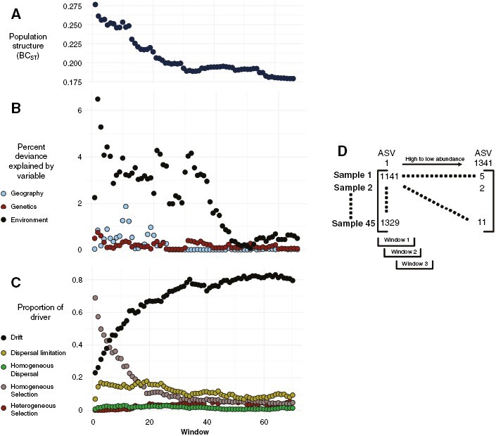
Abundance based sliding window analyses (initial windows are high abundance, final windows are low abundance) of Durvillaea poha microbiomes across southern New Zealand. Rank abundance groups represent windows of 500 ASVs, in step sizes of five, from the most to least abundant ASVs. (A) Amount of population structure associated with the microbiome; high values indicate high structure. (B) Deviance explained by each variable alone based on a generalized dissimilarity model. (C) The relative influence of different ecological factors on the structure of each microbial group. (D) Diagrammatic explanation of window analysis; windows reflect abundances of microbes.
Finally, to understand how selection and neutral processes vary across community abundance, we calculated the contribution of different ecological drivers to community structure using the iCAMP framework (Stegen et al., 2013; Ning et al., 2020). This framework initially calculates phylogenetic turnover as the beta nearest taxon index (BNTI), with values of |BNTI| > 2 indicative of selective/deterministic processes and values of |BNTI| ≤ 2 indicative of stochastic/neutral processes. Then within those neutral processes, taxonomic turnover relative to a randomized null community is calculated as Raup-Crick (RC) index. Values of RC > 0.95 are indicative of dispersal limitation, values of RC < −0.95 are indicative of homogenizing dispersal, and values of |RC| ≤ 0.95 are indicative of ecological drift.
Results
Sequencing summary
Forty-five samples were sequenced successfully for both microbiome and host for D. poha, and 24 samples were sequenced successfully for D. antarctica (Fig. 1). After filtering, 11 390 SNPs were retained for both D. poha and D. antarctica. For microbial samples, an average of 27 231 sequences were present per sample (minimum of 10 180 reads and maximum of 150 423 reads); following decontamination and rarefaction, 1320 ASVs for D. poha and 921 for D. antarctica were retained.
The core microbiome of Durvillaea
We found that the core community for D. poha and D. antarctica comprised 39 and 33 taxa respectively, with 21 taxa shared by both species. Nineteen ASVs were assigned to the genus level (Supplementary Data Table S1). The core microbiome was dominated by Bacteroidia in both D. poha and D. antarctica; however, the former was dominated secondarily by Gammaproteobacteria, whereas the latter was dominated secondarily by Alphaproteobacteria (Supplementary Data Table S2). In D. poha, the core microbiome accounted for, on average, 70.5 % of the community, and for D. antarctica it accounted for 71.1 %.
Algal microbiomes were distinct from the substrate and surrounding seawater communities
Using non-metric dimensionality analyses, we showed that algal microbiomes were distinct from the surrounding seawater and substrate communities. These were distinct from each other based on PERMANOVAs (Fig. 2; Table 1), with seawater, substrate and macroalgal microbiomes all being distinct from each other.
Fig. 2.
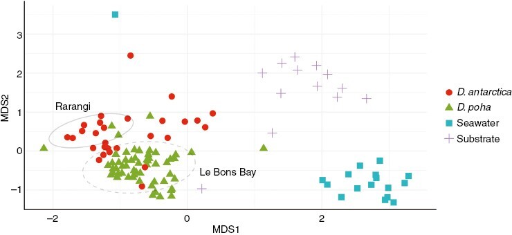
Non-metric dimensionality scaling analyses of marine microbial communities. Green triangles represent samples from specimens genetically identified as Durvillaea poha, and red dots represent Durvillaea antarctica. Blue squares are seawater microbial communities, and grey crosses are substrate samples. The stress value for this non-metric dimensionality analysis is 0.15. Ellipses for Le Bons Bay (dashed) and Rarangi (solid) represent specific locations to demonstrate that locations cluster together. Ellipses are based on 95 % confidence using stat_ellipse in ggplot2 with a normal distribution.
Table 1.
PERMANOVA results from for different sample groups of microbiome data.
| Group | Degrees of freedom | Sum of squares | R 2 | F (P) |
|---|---|---|---|---|
| Sample type (kelp, seawater, substrate) | 2 | 9.05 | 0.22 | 15.70 (0.001) |
| Kelp vs. seawater | 1 | 6.49 | 0.19 | 23.75 (0.001) |
| Kelp vs. substrate | 1 | 3.06 | 0.01 | 10.33 (0.001) |
| Substrate vs. seawater | 1 | 2.64 | 0.23 | 8.40 (0.001) |
| Location (within kelp) | 8 | 9.86 | 0.43 | 6.98 (0.001) |
| Species (within kelp) | 1 | 0.08 | 3.43 × 10⁻³ | 0.44 (0.98) |
We also observed that microbiomes of D. antarctica and D. poha were typically distinct from each other; however, this structure was associated primarily with the collection site. The influence of location on structure appeared to be important, because species outliers (i.e. a sample from D. antarctica clustering within D. poha) were grouped by their location rather than species, alongside significant PERMANOVA results (Table 1).
Microbiome biogeography vs. host biogeography; phylosymbiosis vs. environmental filtering
Broadly, we found evidence for population structure in both the microbiome and host; however, generalized dissimilarity models revealed that the contribution of host genetics was non-significant after considering geographical and environmental distances (Table 2; variable importance for D. poha), suggesting that environmental filtering might lead to population structure in the microbiome rather than host genetics.
Table 2.
Extent of geographical and environmental distance–decay relationships with host genetics and host microbiome data for Durvillaea antarctica and D. poha. Microbiome distance is based on weighted UniFrac to test for phylosymbiosis. Results are from generalized dissimilarity models. In both instances, geographical distance was removed because it explained zero deviance. Significance was assessed via 1000 random permutations. In some instances, P-values cannot be computed owing to insufficient variables to assess the relative importance of variables (indicated by a dash in parentheses). Predictor importance is assessed as the percentage change in deviance explained in models with and without the variable randomized. Nevertheless, the overall model significance is found in the percentage deviance explained column.
| Species | Model (predictor importance; P) | Percentage deviance explained (P) | Total deviance |
|---|---|---|---|
| Durvillaea poha | WuniFrac ~ Environment (–) | 15.44 (<0.001) | 60.8 |
| Genetics ~ Environment (–) | 30.27 (<0.001) | 163.3 | |
| WuniFrac ~ Genetics (0.09 %; <0.001) + Environment (99.03 %; <0.001) | 15.44 (<0.001) | 60.8 | |
| Durvillaea antarctica | WuniFrac ~ Environment (–) | 9.01 (<0.001) | 13.5 |
| Genetics ~ Environment (2.49 %; <0.001) + Geography (4.83 %; <0.001) | 85.38 (<0.001) | 162.5 | |
| WuniFrac ~ Genetics + Environment (–) | 7.13 (<0.001) | 13.5 |
Distance–decay relationships reflect abundance and drivers of community structure, rather than geography
Geographical distance (Fig. 3A) and environmental distance (Fig. 3B) exhibited strong relationships with genetic distance for D. poha, although geographical distance was dropped (Table 3) in variable importance testing owing to an absence of explanatory power relative to geographical distance. There was strong evidence of microbiome distance–decay relationships, with environmental distance (Fig. 3C, D) being a better predictor of microbiome dissimilarity than geographical distance. No significant relationship between host genetic distance and microbiome distance was observed (Fig. 3E). Population structuring (BCST) was stronger in D. poha microbiomes than in those of D. antarctica (Table 3; Supplementary Data Fig. S1).
Fig. 3.

Biogeographical structure of microbiomes and host genetics of Durvillaea poha. Lines and deviance explained derive from the resultant predictive model from the generalized dissimilarity models. (A) Relationship between geographical distance and host genetic distance. (B) Relationship between environmental distance and host genetic distance. (C) Relationship between geographical distance and weighted UniFrac distance. (D) Relationship between environmental distance and weighted UniFrac distance. (E) Relationship between host genetic distance and weighted UniFrac distance; absence of a line indicates that there was no significant relationship between weighted UniFrac distance and host genetic distance.
Table 3.
Beta diversity (Bray–Curtis) values for microbiomes. BCST represents the degree of within vs. between population structure, and beta diversity represents the mean distance to the species centroid. High values of BCST indicate higher levels of population structure (i.e. more distinct population clusters on an ordination).
| Durvillaea antarctica | Durvillaea poha | |||
|---|---|---|---|---|
| BCST | Beta diversity | BCST | Beta diversity | |
| Core | 0.52 | 0.36 | 0.29 | 0.36 |
| Rare | 0.41 | 0.64 | 0.20 | 0.62 |
| Abundant | 0.43 | 0.59 | 0.25 | 0.52 |
| Seawater | 0.95 | 0.14 | 0.80 | 0.18 |
| Substrate | 0.78 | 0.59 | 0.59 | 0.58 |
We hypothesized that the core microbiome would exhibit the least amount of location-related structure, whereas the rare microbiome would have the highest degree of structure, but we observed the opposite (Table 3). Between species of Durvillaea, with regard to Bray–Curtis dissimilarities, there were no differences between species across the core (Z = −0.16, P = 0.87) and rare (Z = 1.3, P = 0.2) microbiomes; however, the abundant microbiomes were significantly different (Z = 2.5, P = 0.01) based on Mann–Whitney U tests.
There were no significant distance–decay relationships in D. antarctica for the core and rare microbiomes; however, the abundant microbiome was strongly associated with environmental distance (Table 4). Likewise, environmental distance–decay relationships were typically strongest for D. poha, with the highest importance and explanatory power relative to other variables.
Table 4.
Deviance explained by variables themselves for generalized dissimilarity between Bray–Curtis distance and geographical, genetic and environmental distances. Values given as NA for variable importance result from such variables being dropped because they explained negligible deviance of in the model. Predictor importance is assessed as the percentage change in deviance explained in models with and without the variable randomized.
| Species | Subcommunity | Variable | Variable importance (P) | Percentage deviance explained by variable alone |
|---|---|---|---|---|
| Durvillaea antarctica | Core | Geography | NA | 0.00 |
| Host genetics | NA | 0.01 | ||
| Environment | NA | 0.00 | ||
| Abundant | Geography | 0 % (1) | 0.01 | |
| Host genetics | NA | 0.57 | ||
| Environment | 3.96 % (<0.001) | 0.05 | ||
| Rare | Geography | NA | 0.00 | |
| Host genetics | NA | 1.7 | ||
| Environment | NA | 0 | ||
| Durvillaea poha | Core | Geography | 3.4 % (<0.001) | 0.49 |
| Host genetics | 0.1 % (<0.001) | 0.02 | ||
| Environment | 53.7 % (<0.001) | 7.77 | ||
| Abundant | Geography | NA | 0.00 | |
| Host genetics | 0.02 % (<0.001) | 0.00 | ||
| Environment | 95.8 % (<0.001) | 1.8 | ||
| Rare | Geography | NA | 0.00 | |
| Host genetics | 0.81 % (<0.001) | 0.18 | ||
| Environment | 94.1 % (<0.001) | 3.18 |
Sliding window analyses revealed that biogeographical structure declined substantially as microbiomes shifted towards a dominance of rarer microbes (Fig. 4A). This decline was associated with reduced strength of environmental and geographical distance–decay relationships (Fig. 4B), alongside a shift towards dominance of neutral processes in the microbiome (Fig. 4C).
As microbial communities shifted towards rarer ASVs, we saw increased contributions of ecological drift to community structure (Fig. 4). Although our data suggest that neutral processes predominantly shape the Durvillaea microbiome, we saw that the influence of selection was mostly limited to the most abundant microbes and that this influence declined with rarity. Likewise, dispersal limitation primarily affected the abundant microbiome, with declining influence of dispersal limitation with rarity.
How do environmental variables affect the microbiome?
There was a notably stronger relationship between geographical distance and genetic distance for the host than there was for the microbiome (Table 2; Fig. 3). We explored these relationships further to attempt to determine the relative influences of geography, host genetics and environmental variables on shaping microbial communities. We found that tidal range was important in shaping both host genetics and microbiome across all categories considered, and that temperature, β-SST and seawater velocity were all frequently important in shaping microbiome and host genetic structure (Table 5).
Table 5.
Relationships between environmental variables and microbiome structure of Durvillaea. Based on partial redundancy analyses of Hellinger-transformed microbiome data, the final model represents the results of stepwise model selection using the ordistep function in vegan.
| Species | Subcommunity | Final model (F; P) | R 2 |
|---|---|---|---|
| Durvillaea antarctica | Core | Tidal range (9.2; <0.001) + Velocity (3.5; <0.001) + β-SST (3.5; 0.001) | 0.43 |
| Abundant | Tidal range (5.1; <0.001) + β-SST (2.3; 0.002) + Velocity (2.5; <0.001) + Salinity (1.7; <0.001) | 0.26 | |
| Rare | Tidal range (1.9; <0.001) + β-SST (1.4; 0.026) + Velocity (1.4; 0.006) | 0.08 | |
| Host genetics | Tidal range (92.8; <0.001) + Velocity (8.5; 0.025) + Temperature (7; <0.001) + β-SST (2.3; 0.1) | 0.83 | |
| Durvillaea poha | Core | Tidal range (8.5; <0.001) + Salinity (5.1; 0.002) + Temperature (4.4; 0.003) + β-SST (5.4; 0.001) | 0.3 |
| Abundant | Temperature (4.1; <0.001) + Tidal range (3.5; <0.001) + Velocity (3.3; <0.001) + β-SST (2.5; 0.004) | 0.18 | |
| Rare | Temperature (2.8; <0.001) + Tidal Range (1.9; <0.001) + Velocity (2.1; <0.001) + β-SST (1.6; 0.003) | 0.09 | |
| Host Genetics | Tidal Range (6.7; <0.001) + Temperature (5.2; <0.001) + Velocity (4.5; <0.001) + Salinity (3.2; <0.001) | 0.26 |
DISCUSSION
Although geographical distance–decay relationships have been noted previously for microbiome biogeography, we show that for Durvillaea microbiomes this relationship is driven primarily by environmental distance. However, for host genetics, there is considerable evidence for joint environmental and geographical distance–decay relationships. These data suggest that the Baas Becking hypothesis (Baas Becking, 1934) that ‘everything is everywhere, the environment selects’ is a useful underlying hypothesis to understand the biogeography of macroalgal microbiomes. We find that the drivers of microbiome assembly transition from selection to neutral processes with abundance, and that abundant microbes show the least biogeographical structure, contrary to our initial hypotheses.
The biogeographical structure of the microbiome results more from environmental filtering than from phylosymbiosis
Although we found that both the hosts and the microbiomes exhibited high levels of population structure, we infer that the drivers of population structure differ between the host genetics and microbiome. Environmental distance decay appears to be the dominant driver of microbiome biogeography, whereas geographical distance decay underpins host phylogeography (Fig. 3). These differences are likely to result from the greater influence of long-term evolutionary processes on host genetics, whereas short-term variations are more likely to drive the structure of the microbiome owing to their relatively shorter time spans and the potential for within-host evolution of microbes (Dapa et al., 2023). Therefore, although the biogeographical patterns are correlated between host genetics and host microbiome, the host genetic patterns arise from long-term evolutionary processes, whereas the microbiome patterns arise from environmental conditions (Fig. 3). The shared biogeographical structure between host and microbiome does not, therefore, reflect phylosymbiosis, but rather environmental filtering.
Our results differ from those of Wood et al. (2022), who inferred strong genetic and geographical distance–decay relationships in the alga Phyllospora comosa but did not consider environmental conditions in examining microbiome variation. Because environmental conditions are known to influence microbiome variation across broad geographical scales (Marzinelli et al., 2015), geographical distance–decay relationships in P. comosa could represent environmental gradients. Without considering environmental conditions, a similar pattern emerges from our data. However, we demonstrate that this pattern results from correlation between environment and geography, with environmental conditions being the underlying driver (Fig. 3).
Distance–decay relationships are driven by abundant bacteria under selection from environmental conditions
Unsurprisingly, the strongest relationships between microbiome and host genetics were within the core and abundant microbiome for D. poha. However, in contrast to our initial hypotheses there was very little evidence of geographical distance decay after accounting for environmental and host genetic distances, suggesting that the Baas Becking hypothesis cannot necessarily be refuted because the strength of environmental distance decay is greatest for high abundance microbes. Such a result is congruent with recent work suggesting that stronger environmental distance–decay relationships are found when communities are dominated by abundant taxa, perhaps resulting from dormant taxa dominating the rare biosphere (Locey et al., 2020).
Contrary to our initial hypotheses, we found that the rarer elements of the microbial communities exhibited the least, rather than the most, population structure (Fig. 4; Table 3). We observed that rarer communities were more predominantly influenced by ecological drift, which, alongside dispersal limitation, is thought to promote differentiation of communities (Gilbert and Levine, 2017). In the case of kelp-associated microbial communities, dispersal limitation and homogeneous selection dominate the abundant microbial communities and decline with abundance, while drift becomes increasingly important. These results contrast with those of sediment communities, where rarer communities are dominated by dispersal limitation and reduced influence of drift (Liu et al., 2023). We suggest that this can be explained by the weaker geographical structure of seawater microbial communities, with seawater samples typically being more similar to each other than kelp samples are to each other. Because drift becomes increasingly important as microbes decline in abundance, the new microbes (which will have reduced abundance initially within the host) must be recruited from the seawater and other algal taxa (Lemay et al., 2018). Recruitment from the environment means that as communities become increasingly drift dominated they are more likely to be representative of the seawater communities and thus, in turn, reflect assemblages of the seawater (Davis et al., 2023).
This potential for environmental microbial diversity to constrain host microbiome diversity does, however, largely assume that kelp-associated microbes are predominantly acquired horizontally rather than vertically. If the latter were the case, then we would expect to see that the population structure of the host would be reflective of that of the microbiome (Griffiths et al., 2019). We suggest that although vertical transmission might play a small role in the community structure of these microbiomes, it is largely outweighed by the contributions of horizontal transmission. Only a small proportion of microbiome variation can be explained by host genetic variation, with the rarest microbes showing the least relationship with host genetics (Fig. 4). Therefore, although vertical acquisition of microbes might occur in Durvillaea, its role is relatively small and occurs primarily in the core microbiome rather than the rare microbiome. The purported dominance of horizontal acquisition of microbes in our data also aligns with expectations owing to our exclusive focus on the external microbiome, which is often assembled via horizontal acquisition of microbes (van Veelen et al., 2017). Finally, across all sliding windows we observed either weak or absent geographical distance–decay relationships (Fig. 4), further supporting the original Baas Becking hypothesis.
Environmental predictability and tidal range are important contributors to microbiome assembly
As with previous research (Marzinelli et al., 2015; Wood et al., 2022), we found that there was a strong influence of environmental conditions on microbiome composition and host genomic variation. Environmental noise, which reflects the degree of short-term environmental variation or the ‘predictability’ over time within a location (Marshall and Burgess, 2015), was frequently implicated as a factor shaping microbiome variation for both D. antarctica and D. poha (Table 5). As a result, lower levels of predictability would be expected to affect the microbiome, because such noise occurs on relatively short time scales (Santillan et al., 2019). These short time scales are ecologically relevant to the microbe owing to their shorter life cycle but would not be anticipated to be a significant factor in shaping host genetics owing to the relatively long life cycle of the host. Such variables might also shape the extent of vertical transmission and perhaps explain the absence of phylosymbiosis patterns within our data. Recent work has shown that low environmental predictability combined with high environmental variation favour lower levels of vertical transmission (Bruijning et al., 2022). Intertidal zones are highly variable owing to tidal action, and marine environments at southern latitudes are less predictable than their Northern Hemisphere counterparts (Di Cecco and Gouhier, 2018). Together, these factors might select against vertical transmission in favour of horizontal transmission and reduce the likelihood of phylosymbiosis.
The influence of tidal range on both microbial and host variation could be attributable to the degree to which a host is exposed to variable environments (Okamoto et al., 2022). With narrower tidal ranges, the population sizes of Durvillaea might be smaller and thus a density effect might be observed, whereby there are fewer kelp to ‘buffer’ the microbiome, leading to higher diversity within these populations (Härer and Rennison, 2023; Pearman et al., 2023). In addition, higher tidal ranges result in more extreme variation in exposure levels, fluctuating from full inundation at high tide to largely out-of-water exposure at low tide. Such changes are likely to result in both selection on the microbiome for tolerant microbes and selection for exposure tolerance in host genetics.
Conclusions
Microbiomes of Durvillaea are distinct from those of the surrounding environment and share many taxa with other macroalgae. Although the biogeographical patterns of both host and microbiome were found to be similar, these patterns arose from different processes, with environmental filtering dominating the microbiome, whereas geographical distance decay best explained host genetic biogeography. Of the environmental variables shaping the microbiome of Durvillaea, environmental predictability was particularly important, alongside tidal range, temperature and current velocity. Finally, we found that rarer components of the microbiome had the least biogeographical structure, despite the expectation that ecological drift would lead to higher geographical structure. We suggest that horizontal transmission probably dominates community assembly for Durvillaea. Given the absence of strong vertical transmission, we suggest that there is a need for better understanding of how holobiont formation occurs in macroalgae and whether vertical transmission makes a contribution. While raising intriguing questions for future studies to address, our findings improve our understanding of how environmental microbial diversity might constrain and shape host diversity, providing valuable insights into the assembly processes and biogeographical structuring of host-associated microbial communities. In particular, the distinct drivers of host and microbiome biogeography might lead to further decoupling under increased anthropogenic pressure owing to the strong role of selection in shaping microbial communities.
SUPPLEMENTARY DATA
Supplementary data are available at Annals of Botany online and consist of the following.
Figure S1: biogeographical structure of microbiomes and host genetics of Durvillaea antarctica. Table S1: core taxa that reached at least genus-level assignment, with functional assignments based on FAPROTAX. Table S2: core taxa at the class level.
ACKNOWLEDGEMENTS
We would like to acknowledge the contributions of Gary Brittenden in sample collection in Le Bons Bay, and the help in laboratory work provided by Linda Groenewegen.
Contributor Information
William S Pearman, Department of Marine Science, University of Otago, New Zealand; Department of Anatomy, School of Biomedical Sciences, University of Otago, New Zealand; Department of Microbiology & Immunology, School of Biomedical Sciences, University of Otago, New Zealand.
Grant A Duffy, Department of Marine Science, University of Otago, New Zealand.
Xiaoyue P Liu, Department of Marine Science, University of Otago, New Zealand.
Neil J Gemmell, Department of Anatomy, School of Biomedical Sciences, University of Otago, New Zealand.
Sergio E Morales, Department of Microbiology & Immunology, School of Biomedical Sciences, University of Otago, New Zealand.
Ceridwen I Fraser, Department of Marine Science, University of Otago, New Zealand.
FUNDING
W.S.P. was funded by a doctoral scholarship from the University of Otago. X.P.L., C.I.F. and G.A.D. were supported by the Marsden Fund Council from Government funding, managed by Royal Society Te Apārangi (MFP-20-UOO-173). C.I.F. was funded by a Rutherford Discovery fellowship (RDF-UOO1803).
CONFLICTS OF INTEREST
The authors have no conflicts of interest to declare.
DATA AVAILABILITY
Because these data originate from a species of significance to the indigenous people of New Zealand, data underlying this paper are available through the Aotearoa Genomic Data Repository (AGDR) at https://doi.org/10.57748/RDXN-1598. The AGDR is a resource for the storage and sharing of genomic data of taonga (culturally significant) species. AGDR was developed by Genomics Aotearoa and New Zealand eScience Infrastructure to provide a secure place for the Aotearoa research community to store and share genomic data within a Māori values context, following the principles of Māori Data Sovereignty.
LITERATURE CITED
- Andrews S. 2010. FastQC: a quality control tool for high throughput sequence data. https://www.bioinformatics.babraham.ac.uk/projects/fastqc/ [computer software] (6 September 2022, date last accessed).
- Assis J, Tyberghein L, Bosch S, Verbruggen H, Serrão EA, De Clerck O.. 2018. Bio-ORACLE v20: extending marine data layers for bioclimatic modelling. Global Ecology and Biogeography 27: 277–284. doi: 10.1111/geb.12693. [DOI] [Google Scholar]
- Azevedo Correia de Souza JM, Suanda SH, Couto PP, Smith RO, Kerry C, Roughan M.. 2023. Moana Ocean Hindcast – a 25-year simulation for New Zealand waters using the Regional Ocean Modeling System (ROMS) v39 model. Geoscientific Model Development 16: 211–231. doi: 10.5194/gmd-16-211-2023. [DOI] [Google Scholar]
- Baas Becking LGM. 1934. Geobiologie of inleiding Tot de Milieukunde. The Hague: WP Van Stockum & Zoon. [Google Scholar]
- Borer ET, Kinkel LL, May G, Seabloom EW.. 2013. The world within: quantifying the determinants and outcomes of a host’s microbiome. Basic and Applied Ecology 14: 533–539. doi: 10.1016/j.baae.2013.08.009. [DOI] [Google Scholar]
- Bruijning M, Henry LP, Forsberg SKG, Metcalf CJE, Ayroles JF.. 2022. Natural selection for imprecise vertical transmission in host–microbiota systems. Nature Ecology & Evolution 6: 77–87. doi: 10.1038/s41559-021-01593-y. [DOI] [PMC free article] [PubMed] [Google Scholar]
- Burns AR, Stephens WZ, Stagaman K, et al. 2016. Contribution of neutral processes to the assembly of gut microbial communities in the zebrafish over host development. The ISME Journal 10: 655–664. doi: 10.1038/ismej.2015.142. [DOI] [PMC free article] [PubMed] [Google Scholar]
- Callahan BJ, McMurdie PJ, Rosen MJ, Han AW, Johnson AJA, Holmes SP.. 2016. DADA2: high-resolution sample inference from Illumina amplicon data. Nature Methods 13: 581–583. doi: 10.1038/nmeth.3869. [DOI] [PMC free article] [PubMed] [Google Scholar]
- Caporaso JG, Lauber CL, Walters WA, et al. 2012. Ultra-high-throughput microbial community analysis on the Illumina HiSeq and MiSeq platforms. The ISME Journal 6: 1621–1624. doi: 10.1038/ismej.2012.8. [DOI] [PMC free article] [PubMed] [Google Scholar]
- Caporaso JG, Ackermann G, Apprill A, et al. 2018. EMP 16S Illumina Amplicon Protocol. https://www.protocols.io/view/emp-16s-illumina-amplicon-protocol-nuudeww
- Clark DR, Underwood GJC, McGenity TJ, Dumbrell AJ.. 2021. What drives study-dependent differences in distance–decay relationships of microbial communities? Global Ecology and Biogeography 30: 811–825. doi: 10.1111/geb.13266. [DOI] [Google Scholar]
- Dapa T, Wong DP, Vasquez KS, Xavier KB, Huang KC, Good BH.. 2023. Within-host evolution of the gut microbiome. Current Opinion in Microbiology 71: 102258. doi: 10.1016/j.mib.2022.102258. [DOI] [PMC free article] [PubMed] [Google Scholar]
- Davis KM, Zeinert L, Byrne A, et al. 2023. Successional dynamics of the cultivated kelp microbiome. Journal of Phycology 59: 538–551. doi: 10.1111/jpy.13329. [DOI] [PubMed] [Google Scholar]
- Davis NM, Proctor DM, Holmes SP, Relman DA, Callahan BJ.. 2018. Simple statistical identification and removal of contaminant sequences in marker-gene and metagenomics data. Microbiome 6: 226. doi: 10.1186/s40168-018-0605-2. [DOI] [PMC free article] [PubMed] [Google Scholar]
- DeRaad DA. 2022. snpfiltr: an R package for interactive and reproducible SNP filtering. Molecular Ecology Resources 22: 2443–2453. doi: 10.1111/1755-0998.13618. [DOI] [PubMed] [Google Scholar]
- DeSantis TZ, Hugenholtz P, Larsen N, et al. 2006. Greengenes, a chimera-checked 16S rRNA gene database and workbench compatible with ARB. Applied and Environmental Microbiology 72: 5069–5072. doi: 10.1128/AEM.03006-05. [DOI] [PMC free article] [PubMed] [Google Scholar]
- de Souza JMAC. 2022. Moana Ocean Hindcast [dataset]. Zenodo. doi: 10.5281/zenodo.5895265. [DOI] [Google Scholar]
- Di Cecco GJ, Gouhier TC.. 2018. Increased spatial and temporal autocorrelation of temperature under climate change. Scientific Reports 8: 14850. doi: 10.1038/s41598-018-33217-0. [DOI] [PMC free article] [PubMed] [Google Scholar]
- Dumbrell AJ, Nelson M, Helgason T, Dytham C, Fitter AH.. 2010. Relative roles of niche and neutral processes in structuring a soil microbial community. The ISME Journal 4: 337–345. doi: 10.1038/ismej.2009.122. [DOI] [PubMed] [Google Scholar]
- Elshire RJ, Glaubitz JC, Sun Q, et al. 2011. A robust, simple genotyping-by-sequencing (GBS) approach for high diversity species. PLoS One 6: e19379. doi: 10.1371/journal.pone.0019379. [DOI] [PMC free article] [PubMed] [Google Scholar]
- Fraser CI, Spencer HG, Waters JM.. 2012. Durvillaea poha sp. nov. (Fucales, Phaeophyceae): a buoyant southern bull-kelp species endemic to New Zealand. Phycologia 51: 151–156. doi: 10.2216/11-47.1. [DOI] [Google Scholar]
- Fraser CI, Morrison AK, Hogg AM, et al. 2018. Antarctica’s ecological isolation will be broken by storm-driven dispersal and warming. Nature Climate Change 8: 704–708. doi: 10.1038/s41558-018-0209-7. [DOI] [Google Scholar]
- Fraser CI, Velásquez M, Nelson WA, Macaya EC, Hay CH.. 2020. The biogeographic importance of buoyancy in macroalgae: a case study of the southern bull-kelp genus Durvillaea (Phaeophyceae), including descriptions of two new species. Journal of Phycology 56: 23–36. doi: 10.1111/jpy.12939. [DOI] [PubMed] [Google Scholar]
- Fraser CI, Dutoit L, Morrison AK, et al. 2022. Southern Hemisphere coasts are biologically connected by frequent, long-distance rafting events. Current Biology: CB 32: 3154–3160.e3. doi: 10.1016/j.cub.2022.05.035. [DOI] [PubMed] [Google Scholar]
- Gilbert B, Levine JM.. 2017. Ecological drift and the distribution of species diversity. Proceedings Biological Sciences 284: 20170507. doi: 10.1098/rspb.2017.0507. [DOI] [PMC free article] [PubMed] [Google Scholar]
- Gillingham MAF, Béchet A, Cézilly F, et al. 2019. Offspring microbiomes differ across breeding sites in a panmictic species. Frontiers in Microbiology 10: 35. doi: 10.3389/fmicb.2019.00035. [DOI] [PMC free article] [PubMed] [Google Scholar]
- Graco-Roza C, Aarnio S, Abrego N, et al. 2022. Distance decay 20 – a global synthesis of taxonomic and functional turnover in ecological communities. Global Ecology and Biogeography 31: 1399–1421. doi: 10.1111/geb.13513. [DOI] [PMC free article] [PubMed] [Google Scholar]
- Griffiths SM, Antwis RE, Lenzi L, et al. 2019. Host genetics and geography influence microbiome composition in the sponge Ircinia campana. The Journal of Animal Ecology 88: 1684–1695. doi: 10.1111/1365-2656.13065. [DOI] [PMC free article] [PubMed] [Google Scholar]
- Guillou L, Bachar D, Audic S, et al. 2013. The Protist Ribosomal Reference database (PR2): a catalog of unicellular eukaryote Small Sub-Unit rRNA sequences with curated taxonomy. Nucleic Acids Research 41: D597–D604. doi: 10.1093/nar/gks1160. [DOI] [PMC free article] [PubMed] [Google Scholar]
- Härer A, Rennison DJ.. 2023. The biogeography of host-associated bacterial microbiomes: revisiting classic biodiversity patterns. Global Ecology and Biogeography 32: 931–944. doi: 10.1111/geb.13675. [DOI] [Google Scholar]
- Hazard C, Gosling P, van der Gast CJ, Mitchell DT, Doohan FM, Bending GD.. 2013. The role of local environment and geographical distance in determining community composition of arbuscular mycorrhizal fungi at the landscape scale. The ISME Journal 7: 498–508. doi: 10.1038/ismej.2012.127. [DOI] [PMC free article] [PubMed] [Google Scholar]
- Heys C, Cheaib B, Busetti A, et al. 2020. Neutral processes dominate microbial community assembly in Atlantic salmon, Salmo salar. Applied and Environmental Microbiology 86: e02283-19. doi: 10.1128/AEM.02283-19. [DOI] [PMC free article] [PubMed] [Google Scholar]
- Jombart T, Ahmed I.. 2011. adegenet 13-1: new tools for the analysis of genome-wide SNP data. Bioinformatics 27: 3070–3071. doi: 10.1093/bioinformatics/btr521. [DOI] [PMC free article] [PubMed] [Google Scholar]
- Joung YS, Ge Z, Buie CR.. 2017. Bioaerosol generation by raindrops on soil. Nature Communications 8: 14668. doi: 10.1038/ncomms14668. [DOI] [PMC free article] [PubMed] [Google Scholar]
- Kamvar ZN, Tabima JF, Grünwald NJ.. 2014. Poppr: an R package for genetic analysis of populations with clonal, partially clonal, and/or sexual reproduction. PeerJ 2: e281. doi: 10.7717/peerj.281. [DOI] [PMC free article] [PubMed] [Google Scholar]
- Lemay MA, Martone PT, Keeling PJ, et al. 2018. Sympatric kelp species share a large portion of their surface bacterial communities. Environmental Microbiology 20: 658–670. doi: 10.1111/1462-2920.13993. [DOI] [PubMed] [Google Scholar]
- Lemay MA, Davis KM, Martone PT, Parfrey LW.. 2021. Kelp-associated microbiota are structured by host anatomy. Journal of Phycology 57: 1119–1130. doi: 10.1111/jpy.13169. [DOI] [PubMed] [Google Scholar]
- Li H. 2013. Aligning sequence reads, clone sequences and assembly contigs with BWA-MEM. arXiv:1303.3997 [q-Bio]. http://arxiv.org/abs/1303.3997
- Li S, Wang P, Chen Y, et al. 2020. Island biogeography of soil bacteria and fungi: similar patterns, but different mechanisms. The ISME Journal 14: 1886–1896. doi: 10.1038/s41396-020-0657-8. [DOI] [PMC free article] [PubMed] [Google Scholar]
- Lim SJ, Bordenstein SR.. 2020. An introduction to phylosymbiosis. Proceedings Biological Sciences 287: 20192900. doi: 10.1098/rspb.2019.2900. [DOI] [PMC free article] [PubMed] [Google Scholar]
- Linck E, Battey CJ.. 2019. Minor allele frequency thresholds strongly affect population structure inference with genomic data sets. Molecular Ecology Resources 19:639–647. [DOI] [PubMed] [Google Scholar]
- Liu X, Li H, Song W, Tu Q.. 2023. Distinct ecological mechanisms drive the spatial scaling of abundant and rare microbial taxa in a coastal sediment. Journal of Biogeography 50: 909–919. doi: 10.1111/jbi.14584. [DOI] [Google Scholar]
- Locey KJ, Muscarella ME, Larsen ML, Bray SR, Jones SE, Lennon JT.. 2020. Dormancy dampens the microbial distance–decay relationship. Philosophical Transactions of the Royal Society B: Biological Sciences 375: 20190243. doi: 10.1098/rstb.2019.0243. [DOI] [PMC free article] [PubMed] [Google Scholar]
- Lozupone CA, Hamady M, Kelley ST, Knight R.. 2007. Quantitative and qualitative β diversity measures lead to different insights into factors that structure microbial communities. Applied and Environmental Microbiology 73: 1576–1585. doi: 10.1128/AEM.01996-06. [DOI] [PMC free article] [PubMed] [Google Scholar]
- Madden T. 2013. The BLAST sequence analysis tool. Bethesda, Maryland: National Center for Biotechnology Information (USA). [Google Scholar]
- Marshall DJ, Burgess SC.. 2015. Deconstructing environmental predictability: seasonality, environmental colour and the biogeography of marine life histories. Ecology Letters 18: 174–181. doi: 10.1111/ele.12402. [DOI] [PubMed] [Google Scholar]
- Martiny JBH, Bohannan BJM, Brown JH, et al. 2006. Microbial biogeography: putting microorganisms on the map. Nature Reviews Microbiology 4: 102–112. doi: 10.1038/nrmicro1341. [DOI] [PubMed] [Google Scholar]
- Marzinelli EM, Campbell AH, Zozaya Valdes E, et al. 2015. Continental-scale variation in seaweed host-associated bacterial communities is a function of host condition, not geography. Environmental Microbiology 17: 4078–4088. doi: 10.1111/1462-2920.12972. [DOI] [PubMed] [Google Scholar]
- Mazel F, Davis KM, Loudon A, Kwong WK, Groussin M, Parfrey LW.. 2018. Is host filtering the main driver of phylosymbiosis across the tree of life? mSystems 3: e00097-18. doi: 10.1128/mSystems.00097-18. [DOI] [PMC free article] [PubMed] [Google Scholar]
- McMurdie PJ, Holmes S.. 2013. phyloseq: an R Package for reproducible interactive analysis and graphics of microbiome census data. PLoS One 8: e61217. doi: 10.1371/journal.pone.0061217. [DOI] [PMC free article] [PubMed] [Google Scholar]
- Meyer KM, Memiaghe H, Korte L, Kenfack D, Alonso A, Bohannan BJM.. 2018. Why do microbes exhibit weak biogeographic patterns? The ISME Journal 12: 1404–1413. doi: 10.1038/s41396-018-0103-3. [DOI] [PMC free article] [PubMed] [Google Scholar]
- Minich JJ, Morris MM, Brown M, et al. 2018. Elevated temperature drives kelp microbiome dysbiosis, while elevated carbon dioxide induces water microbiome disruption. PLoS One 13: e0192772. doi: 10.1371/journal.pone.0192772. [DOI] [PMC free article] [PubMed] [Google Scholar]
- Mony C, Uroy L, Khalfallah F, Haddad N, Vandenkoornhuyse P.. 2022. Landscape connectivity for the invisibles. Ecography 2022: e06041. doi: 10.1111/ecog.06041. [DOI] [Google Scholar]
- Nekola JC, White PS.. 1999. The distance decay of similarity in biogeography and ecology. Journal of Biogeography 26: 867–878. doi: 10.1046/j.1365-2699.1999.00305.x. [DOI] [Google Scholar]
- Ning D, Yuan M, Wu L, et al. 2020. A quantitative framework reveals ecological drivers of grassland microbial community assembly in response to warming. Nature Communications 11: 4717. doi: 10.1038/s41467-020-18560-z. [DOI] [PMC free article] [PubMed] [Google Scholar]
- Obst M. 2017. Globala tidvattensvariabler. Global tide variables (1.0) [dataset]. University of Gothenburg. doi: 10.5879/C49R-X993 [DOI] [Google Scholar]
- Okamoto N, Keeling PJ, Leander BS, Tai V.. 2022. Microbial communities in sandy beaches from the three domains of life differ by microhabitat and intertidal location. Molecular Ecology 31: 3210–3227. doi: 10.1111/mec.16453. [DOI] [PubMed] [Google Scholar]
- Oksanen J, Blanchet FG, Kindt R, et al. 2010. Vegan: community ecology package. R package version 1.17-4. https://cran.r-project.org/web/packages/vegan (1 September 2023, date last accessed).
- Özkurt E, Fritscher J, Soranzo N, et al. 2022. LotuS2: an ultrafast and highly accurate tool for amplicon sequencing analysis. Microbiome 10: 176. doi: 10.1186/s40168-022-01365-1. [DOI] [PMC free article] [PubMed] [Google Scholar]
- Pante E, Simon-Bouhet B.. 2013. marmap: a package for importing, plotting and analyzing bathymetric and topographic data in R. PLoS One 8: e73051. doi: 10.1371/journal.pone.0073051. [DOI] [PMC free article] [PubMed] [Google Scholar]
- Pearman WS, Morales SE, Vaux F, Gemmell N, Fraser CI.. 2023. Differences in density: taxonomic but not functional diversity in seaweed microbiomes affected by an earthquake (p 20230208527737). bioRxiv. doi: 10.1101/2023.02.08.527737. [DOI] [Google Scholar]
- Perez-Lamarque B, Krehenwinkel H, Gillespie RG, Morlon H.. 2022. Limited evidence for microbial transmission in the phylosymbiosis between Hawaiian spiders and their microbiota. mSystems 7: e0110421. doi: 10.1128/msystems.01104-21. [DOI] [PMC free article] [PubMed] [Google Scholar]
- Peters JC, Waters JM, Dutoit L, Fraser CI.. 2020. SNP analyses reveal a diverse pool of potential colonists to earthquake-uplifted coastlines. Molecular Ecology 29: 149–159. doi: 10.1111/mec.15303. [DOI] [PubMed] [Google Scholar]
- Qiu Z, Coleman MA, Provost E, et al. 2019. Future climate change is predicted to affect the microbiome and condition of habitat-forming kelp. Proceedings Biological Sciences 286: 20181887. doi: 10.1098/rspb.2018.1887. [DOI] [PMC free article] [PubMed] [Google Scholar]
- Quast C, Pruesse E, Yilmaz P, et al. 2013. The SILVA ribosomal RNA gene database project: improved data processing and web-based tools. Nucleic Acids Research 41: D590–D596. doi: 10.1093/nar/gks1219. [DOI] [PMC free article] [PubMed] [Google Scholar]
- Ritari J, Salojärvi J, Lahti L, de Vos WM.. 2015. Improved taxonomic assignment of human intestinal 16S rRNA sequences by a dedicated reference database. BMC Genomics 16: 1056. doi: 10.1186/s12864-015-2265-y. [DOI] [PMC free article] [PubMed] [Google Scholar]
- Rochette NC, Rivera-Colón AG, Catchen JM.. 2019. Stacks 2: analytical methods for paired-end sequencing improve RADseq-based population genomics. Molecular Ecology 28: 4737–4754. doi: 10.1111/mec.15253. [DOI] [PubMed] [Google Scholar]
- Santillan E, Seshan H, Constancias F, Drautz-Moses DI, Wuertz S.. 2019. Frequency of disturbance alters diversity, function, and underlying assembly mechanisms of complex bacterial communities. NPJ Biofilms and Microbiomes 5: 8. doi: 10.1038/s41522-019-0079-4. [DOI] [PMC free article] [PubMed] [Google Scholar]
- Shade A, Stopnisek N.. 2019. Abundance-occupancy distributions to prioritize plant core microbiome membership. Current Opinion in Microbiology 49: 50–58. doi: 10.1016/j.mib.2019.09.008. [DOI] [PubMed] [Google Scholar]
- Sieber M, Traulsen A, Schulenburg H, Douglas AE.. 2021. On the evolutionary origins of host–microbe associations. Proceedings of the National Academy of Sciences of the United States of America 118: e2016487118. doi: 10.1073/pnas.2016487118. [DOI] [PMC free article] [PubMed] [Google Scholar]
- Stegen JC, Lin X, Fredrickson JK, et al. 2013. Quantifying community assembly processes and identifying features that impose them. The ISME Journal 7: 2069–2079. doi: 10.1038/ismej.2013.93. [DOI] [PMC free article] [PubMed] [Google Scholar]
- Sutherland J, Bell T, Trexler RV, Carlson JE, Lasky JR.. 2022. Host genomic influence on bacterial composition in the switchgrass rhizosphere. Molecular Ecology 31: 3934–3950. doi: 10.1111/mec.16549. [DOI] [PMC free article] [PubMed] [Google Scholar]
- Tesson SVM, Okamura B, Dudaniec RY, et al. 2015. Integrating microorganism and macroorganism dispersal: modes, techniques and challenges with particular focus on co-dispersal. Écoscience 22: 109–124. doi: 10.1080/11956860.2016.1148458. [DOI] [Google Scholar]
- Tong X, Leung MHY, Wilkins D, Cheung HHL, Lee PKH.. 2019. Neutral processes drive seasonal assembly of the skin mycobiome. mSystems 4: e00004-19. doi: 10.1128/mSystems.00004-19. [DOI] [PMC free article] [PubMed] [Google Scholar]
- Troussellier M, Escalas A, Bouvier T, Mouillot D.. 2017. Sustaining rare marine microorganisms: macroorganisms as repositories and dispersal agents of microbial diversity. Frontiers in Microbiology 8: 947. doi: 10.3389/fmicb.2017.00947. [DOI] [PMC free article] [PubMed] [Google Scholar]
- van Veelen HPJ, Falcao Salles J, Tieleman BI.. 2017. Multi-level comparisons of cloacal, skin, feather and nest-associated microbiota suggest considerable influence of horizontal acquisition on the microbiota assembly of sympatric woodlarks and skylarks. Microbiome 5: 156. doi: 10.1186/s40168-017-0371-6. [DOI] [PMC free article] [PubMed] [Google Scholar]
- Vargas S, Leiva L, Wörheide G.. 2021. Short-term exposure to high-temperature water causes a shift in the microbiome of the common aquarium sponge Lendenfeldia chondrodes. Microbial Ecology 81: 213–222. doi: 10.1007/s00248-020-01556-z. [DOI] [PMC free article] [PubMed] [Google Scholar]
- Vasseur DA, Yodzis P.. 2004. The color of environmental noise. Ecology 85: 1146–1152. doi: 10.1890/02-3122. [DOI] [Google Scholar]
- Vaux F, Parvizi E, Craw D, Fraser CI, Waters JM.. 2022. Parallel recolonizations generate distinct genomic sectors in kelp following high-magnitude earthquake disturbance. Molecular Ecology 31: 4818–4831. doi: 10.1111/mec.16535. [DOI] [PMC free article] [PubMed] [Google Scholar]
- Velásquez M, Fraser CI, Nelson WA, Tala F, Macaya EC.. 2020. Concise review of the genus Durvillaea Bory de Saint-Vincent, 1825. Journal of Applied Phycology 32: 3–21. doi: 10.1007/s10811-019-01875-w. [DOI] [Google Scholar]
- Wilson LJ, Weber XA, King TM, Fraser CI.. 2016. DNA extraction techniques for genomic analyses of macroalgae. In: Hu Z-M, Fraser C, eds. Seaweed phylogeography: adaptation and evolution of seaweeds under environmental change. Dordrecht, Netherlands: Springer Netherlands, 363–386. doi: 10.1007/978-94-017-7534-2_15 [DOI] [Google Scholar]
- Wood G, Steinberg PD, Campbell AH, Vergés A, Coleman MA, Marzinelli EM.. 2022. Host genetics, phenotype and geography structure the microbiome of a foundational seaweed. Molecular Ecology 31: 2189–2206. doi: 10.1111/mec.16378. [DOI] [PMC free article] [PubMed] [Google Scholar]
Associated Data
This section collects any data citations, data availability statements, or supplementary materials included in this article.
Supplementary Materials
Data Availability Statement
Because these data originate from a species of significance to the indigenous people of New Zealand, data underlying this paper are available through the Aotearoa Genomic Data Repository (AGDR) at https://doi.org/10.57748/RDXN-1598. The AGDR is a resource for the storage and sharing of genomic data of taonga (culturally significant) species. AGDR was developed by Genomics Aotearoa and New Zealand eScience Infrastructure to provide a secure place for the Aotearoa research community to store and share genomic data within a Māori values context, following the principles of Māori Data Sovereignty.