Understanding change in benthic marine systems

Abstract

Background

The unprecedented influence of human activities on natural ecosystems in the 21st century has resulted in increasingly frequent large-scale changes in ecological communities. This has heightened interest in understanding such changes and effective means to manage them. Accurate interpretation of state changes is challenging because of difficulties translating theory to empirical study, and most theory emphasizes systems near equilibrium, which may not be relevant in rapidly changing environments.

Scope

We review concepts of long-transient stages and phase shifts between stable community states, both smooth, continuous and discontinuous shifts, and the relationships among them. Three principal challenges emerge when applying these concepts. The first is how to interpret observed change in communities – distinguishing multiple stable states from long transients, or reversible shifts in the phase portrait of single attractor systems. The second is how to quantify the magnitudes of three sources of variability that cause switches between community states: (1) ‘noise’ in species’ abundances, (2) ‘wiggle’ in system parameters and (3) trends in parameters that affect the topography of the basin of attraction. The third challenge is how variability of the system shapes evidence used to interpret community changes. We outline a novel approach using critical length scales to potentially address these challenges. These concepts are highlighted by a review of recent examples involving macroalgae as key players in marine benthic ecosystems.

Conclusions

Real-world examples show three or more stable configurations of ecological communities may exist for a given set of parameters, and transient stages may persist for long periods necessitating their respective consideration. The characteristic length scale (CLS) is a useful metric that uniquely identifies a community ‘basin of attraction’, enabling phase shifts to be distinguished from long transients. Variabilities of CLSs and time series data may likewise provide proactive management measures to mitigate phase shifts and loss of ecosystem services. Continued challenges remain in distinguishing continuous from discontinuous phase shifts because their respective dynamics lack unique signatures.

INTRODUCTION

Large-scale changes in the structure of ecological communities (i.e. species composition, relative abundance, distribution, diversity, organizing processes) can occur in a short time in response to acute pulse, or chronic press, events and persist for long periods. The late 20th and early 21st centuries have been increasingly marked by dramatic changes of communities in natural ecosystems. Transitions of redwood or oak hardwood forests to woody shrublands have been linked to increased severity of wildfires associated with pathogenic infection by a water mould that increases the fuel load in California forests (Cobb et al., 2012; Metz et al., 2013). Nutrient loading of oligotrophic, shallow freshwater lakes beyond a critical threshold increases phytoplankton biomass and turbidity that adversely affect the community of submerged aquatic vegetation and zooplankton that are key to maintaining the clear water state (Scheffer and Carpenter, 2003; Carpenter et al., 2008). In the oceans, many coral reefs switch among coral and algal, soft coral or sponge-dominated communities (Hughes, 1994; Dudgeon et al., 2010; Pawlik, 2011). Macroalgal forests around the globe have been observed to switch among kelp (or other macroalgae) and algal turf, or sea urchin/crustose coralline-dominated states (Ling et al., 2009, 2015; Filbee-Dexter and Scheibling, 2014; Strain et al., 2014; Krumhansl et al., 2016; Filbee-Dexter and Wernberg, 2018). Some temperate rocky shore communities switch between macroalgal- or mussel-dominated states (Petraitis et al., 2009; Petraitis and Dudgeon, 2015a; Dudgeon and Petraitis, 2022). Particularly in this period of rapidly changing climate, ecologists need to determine both the causes (i.e. anthropogenic or not) and consequences (e.g. potential loss of ecosystem services) of such changes. This is important not only to advance fundamental understanding of how natural communities assemble and collapse or otherwise change, but also to convey understanding to managers and policy-makers in the context of useful management guidance.

This is easier said than done. Ecologists face challenges in interpreting accurately what observed changes of community state represent. A change of state of a community may represent a transient (successional) stage from which the prior, or a new, asymptotic (equilibrium) community will emerge. The state change may represent a fluctuating or oscillatory behaviour within a single long-term domain of attraction. Long transients are not uncommon and may appear stable and persist over a long time (Hastings et al., 2018) if they are detected at all. They pose an interpretive challenge of recognizing and distinguishing them from asymptotic states (Morozov et al., 2020). Likewise, there are challenges of interpreting observed changes of community state near or at a different (new) stable equilibrium. Whether the change is a response to a persistent change in system parameters (e.g. environmental), a temporary extrinsic perturbation to state variables (without persistent environmental change) or perhaps both can be difficult to discern. The consequences of a change in community state are similarly crucial to determine, especially where there is reliance on ecosystem services provided. The central issues here are whether changes of community state are transient or persistent and whether they can be reversed (assuming the will and resources to restore a desired former state exist) commensurate with the efforts to restore environmental conditions that prevailed prior to the shift. Ecosystem managers face great challenges if community restoration requires that environmental conditions be reversed well beyond those that precipitated collapse in the first place. With respect to transient stages, managers must recognize them as such, as well as the asymptotic state to which they belong, and decide whether investment of resources to either reverse conditions or accelerate succession is justified, presumably depending upon the anticipated longevity of the transient and expected loss of ecosystem services. Accurately inferring ecological phenomena from outcomes of empirical investigation can be as vexing to ecologists as they are important to understanding and managing natural ecosystems in the face of rapid environmental change.

A large body of theory developed over decades provides guidance for interpreting possible outcomes and explanation for sudden, large changes of community state. Catastrophe theory (Arnol’d, 1992; Thom, 1975; Zeeman, 1976) and the theory of alternative stable states (Lewontin, 1969; May, 1977) describe stable, asymptotic behaviours of systems and their possible outcomes, which have been a focus of ecologists and the topic of several reviews (e.g. Connell and Sousa, 1983; Peterson, 1984, Knowlton, 1992; Scheffer et al., 2001; Petraitis and Dudgeon, 2004, 2015b; Schröder et al., 2005; Dudgeon et al., 2010). Given the pace of environmental change and the need to manage desirable outcomes of sudden, large-scale changes in ecosystems, recent emphasis has used dynamical systems theory to develop a systematic framework for studying transient (non-asymptotic) behaviour of ecological systems (Hastings et al., 2018, 2021; Morozov et al., 2020; Francis et al., 2021). Collectively, these theories have provided key insights to guide interpretation of ecological dynamics. Nevertheless, as discussed by Petraitis (2013) and Petraitis and Dudgeon (2015b), navigation by empiricists of the maps provided by theory remain a challenge in terms of identifying and translating useful facets of theory appropriately such that they can be applied to experimental and/or sampling designs of empirical tests.

The principal aim of this contribution is to compare essential attributes of theories of asymptotic and transient dynamics that summarizes the state of current thinking in ecology to serve as a practical guide to the interpretation of community dynamics in natural ecosystems. We begin by defining our terminology and review recent examples of sudden, large-scale changes of community state in coastal marine ecosystems in which macroalgae form a foundational functional group by providing energy from their production and habitat from their size and structure. We summarize remaining challenges faced by empiricists interpreting ecological dynamics in the context of theory. Methods are proposed to quantitatively characterize the magnitudes of sources of variability that can cause abrupt changes of community state and shape the nature of evidence useful for interpreting outcomes of changes. Finally, we review an approach using critical length scales to: (1) distinguish phase shifts from ecological transients of a resident assemblage, (2) distinguish among community states of an ecosystem and (3) enable assignment of transient ecological stages to corresponding asymptotic stable states.

CHARACTERIZING CHANGE IN COMMUNITY STRUCTURE

Terminology

Despite attempts by several authors to provide a tightly defined and precise lexicon (e.g. Schröder et al., 2005; Dudgeon et al., 2010; Petraitis, 2013), the spaghetti of terminology used by ecologists to describe change in community composition (and sometimes, by implication, change in function) has caused confusion, been inconsistent and even been contradictory.

Regime shift and phase shift have been used synonymously to indicate a large and (usually) persistent shift in composition at the community level, with researchers of open-water systems tending to use the former while the latter is often used to describe change in community structure on reefs and other benthic systems (e.g. Conversi et al., 2015). Here we use ‘phase shift’, in part because its historical use also permits us to differentiate between continuous and discontinuous phase shift, which is an important distinction (Fig. 1). Also, there are several different definitions of regime shift in the literature, and its definition often requires a time scale of change, i.e. a rapid shift (e.g. Conversi et al., 2015; Pedersen et al., 2020). Particularly with the accumulating effects of climate change, empirical observations of community change in marine systems often record relatively abrupt shifts (e.g. Hare and Mantua, 2000), but there is no theoretical requirement that a phase shift be rapid or sudden (Petraitis and Dudgeon, 2015b).

Fig. 1.

Schematic representing (A) various trajectories of continuous phase shift and (B) discontinuous phase shift. Continuous phase shifts (A) may be linear or non-linear, and have thresholds or tipping points, or not. For discontinuous phase shifts (B) there are forwards and backwards tipping points between which lie environmental conditions able to support multiple stable states and which defines an ecological hysteresis. (C) Two ‘controlling’ environmental variables can yield a catastrophe fold (or cusp) in the equilibrium surface so that depending on the value of Variable 2, the state response to changes in Variable 1 can represent either a continuous or discontinuous phase shift. Different coloured pathways with arrows depict community trajectories between alternative stable states. The manifold surface contains the potential for hysteresis by virture of its shape, but hysteresis is not detectable from the actual path the system takes. The Green curve shows a one-jump path. Grey arrows depict pathways crossing the cusp that diverge into alternative stable states from different initial conditions. (D) Folding of the equilibrium phase surface in a way that supports three different stable states in particular areas of environmental parameter space (the example here shown as stable states X, Y and Z at the same point of parameter space). The surface, which appears as one cusp atop another, is a slice taken from the butterfly catastrophe, which contains four folds and three cusps, and shown here with respect to values of two control parameters with the other two parameters held constant. More than three stable states are possible in the one model. After Scheffer et al. (2001) and Petraitis (2013).

Importantly, a continuous phase shift is associated with only a single stable state in any environment (Fig. 1A). In contrast, by definition, discontinuous phase shifts, sometimes referred to as catastrophic shifts, arise from alternative (aka multiple) stable states over some range of environmental conditions (Fig. 1B). The distinction between a continuous and discontinuous shift is important because they connote vastly different challenges for managers. In a continuous phase shift, whether linear or not, managers can return a community to a previous configuration to the extent that environmental conditions can be returned to previous levels. However, in the case of a discontinuous phase shift, the ecological system does not return to its previous configuration once conditions are returned to values characteristic of the pre-shift environment; it remains stubbornly in its ‘new’ stable configuration. This is the essence of hysteresis: trajectories of a community among equilibria do not follow the same path in ‘forward’ and ‘backward’ shifts (Fig. 1B). Thus, in this circumstance ‘prevention’ is much easier (and thus cheaper) than ‘cure’; discontinuous phase shift is a manager’s nightmare.

Perhaps no less of a nightmare is the phenomenon of long-transient ecological stages. Given the pace of climate change and associated changes in ecological communities, several authors have persuasively argued that applying theory of asymptotic community states that may not occur until well into the future is irrelevant to the demands for management of rapidly changing ecosystems far from equilibrium in the present (Hastings et al., 2018, 2021; Morozov et al., 2020; Francis et al., 2021). Instead, theory describing dynamic behaviours of transient successional stages to accompany that of asymptotic states is required. Here, we follow the terminology of Hastings et al. (2018, 2021) and Morozov et al. (2020) to define and describe transient phenomena. Transient ecological stages are those that do not persist indefinitely (i.e. by definition they are not asymptotic, though they may be long) and their replacement occurs without any forcing (e.g. without change in parameters or perturbations to state variables). Long transients are those that last longer than the characteristic timescales of community dynamics and generation times of long-lived species in the system. Thus, they probably appear to be a stable state to the observer and the manager’s nightmare in this case is the difficulty of distinguishing the long transient as such, recognizing the basin of attraction to which the transient belongs and deciding what, if any, action should be taken given an unknown longevity that may last many years. An added difficulty is the potential for multiple transient stages in a successional sequence that eventually leads to an asymptotic state.

Theory and practice

The challenge for ecologists and real-world managers, therefore, is how to interpret and respond to (or not) observed community change. Despite the differences between long transient stages versus a stable configuration, and between continuous and discontinuous phase shifts, there remain difficulties in distinguishing among them from a practical perspective. For example, on the one hand, while a phase shift is often persistent, it need not be; the drivers of a continuous phase shift might be reversed, returning the system to its previous configuration. On the other, transient ecological stages may persist for very long periods and appear stable owing to their longevity, and the eventual asymptotic state may be uncertain.

Long transient stages

Long transients arise both from the collective traits of species in the assemblage and from where the ecosystem lies along axes of environmental condition (i.e. parameter values; Hastings et al., 2018; Morozov et al., 2020). Traits of species and ecosystems that make long transients a common occurrence include (1) occupation by long-lived species, (2) species with very different generation times (some fast, others slow), (3) time lags, (4) spatial structure and/or (5) environmental stochasticity (Morozov et al., 2020; Hastings et al., 2021); basically, commonly occurring, realistic features of many natural ecosystems.

Long transients also occur when an ecosystem lies in the proximity of steep thresholds, folds, unstable equilibria or cusps in the equilibrial surface. Figure 2 is Fig. 1B modified to map the loci of long-transient phenomena relative to the equilibria. The inset panels depict the ball and cup model of the surface potential characterizing ecosystem resilience at points a, b and c representing different environmental conditions. As the environment changes (beginning at ‘a’ and moving left to right), the potential surface flattens, greatly slowing the recovery time of community state to perturbation. As the system crosses ‘c’ a stable equilibrium is lost and the surface becomes flat there and almost flat in the vicinity just beyond. The subsequent slowing where there used to be a stable equilibrium, named a ‘ghost attractor’, is an important cause of long transients because flat potential surfaces imply very slow ecological dynamics (Hastings et al., 2018). Another feature associated with long transients is unstable equilibria, or equilibria of the saddle type. In this case, the potential surface in the vicinity of a saddle can likewise be very flat such that the dynamics of a system entrained within it move very slowly causing a long transient named a ‘crawl-by’ (shaded region). Importantly, the traits of an ecosystem, such as stochasticity, and its position with respect to features of a basin of attraction can interact with one another to affect the dynamics of long transients, including increasing or decreasing their duration (Hastings et al., 2021).

Fig. 2.

The schematic curve of Fig. 1B including inset panels showing the potential of the system (V) at various points along the curve of equilibria. Curved blue lines give the equilibria for the state variable at different levels of an environmental condition. Solid lines show stable states; dashed lines show unstable states. Inset panels are the cup-and-ball models; note how the potential surface flattens as the system approaches and passes a fold (points a, b and c). Point c is a ghost attractor because the cup shown as point b disappears. The shaded purple region shows a crawl-by in the vicinity of the unstable equilibria (saddle region) where, like ghost attractors, dynamics slow down causing long transients (Hastings et al., 2018).

Limitations of metrics to identify phase shifts

Continuous phase shifts can also show largely overlapping signatures with discontinuous phase shifts in a way that hampers correct identification of the type of phase shift. This stems from the fact that they are not mutually exclusive alternative models. On the contrary, both occur within the single model known as a cusp catastrophe (Fig. 1C), which is described by a single state variable and two parameters that join the smooth continuous shift with discontinuous jumps (Zeeman, 1976; Petraitis, 2013; Petraitis and Dudgeon, 2015b). Like discontinuous jumps (i.e. catastrophes), continuous phase shifts may show tipping points or thresholds at which unexpectedly abrupt changes of state may happen, yet in neither case is it implied that the shift is necessarily rapid. The approach to the new equilibria in both cases may be very slow (Petraitis, 2013; Petraitis and Dudgeon, 2015b; Hastings et al., 2018; Morozov et al., 2020). Thus, rates of change of state are not useful as evidence of the potential number of asymptotic states for an environment.

Recently, attention has focused on the behaviour of state variables associated with equilibria near a cusp or fold where the potential surface flattens and dynamics slow. The concept of early warning signals (EWS) is worth considering briefly if only because managers would be in a stronger position if there were reliable EWS that preceded phase shifts in macroalgal systems. Most work on EWS has been with model systems, and focused on the phenomenon of ‘critical slowing down’ and its related properties of increased variance, autocorrelation and non-linear response of state variables as a system approaches a tipping point (Poston and Stewart, 1978; Gilmore, 1981; Scheffer et al., 2009, 2012; Dakos et al., 2015; Clements and Ozgul, 2018). Critical slowing down refers to a behaviour where responses to perturbations and the tendency of a system to return to a previous state slow down, decreasing resilience near tipping points. However, while it has been claimed as a generic property of phase (or regime) shifts, it is clear that critical slowing down is completely absent in some ecological models manifesting discontinuous phase shifts and which show so-called ‘silent catastrophes’ (Hastings and Wysham, 2010; Boerlijst et al., 2013). Completely different approaches to the question of EWS, for example based on information theoretic statistics such as global transfer entropy (Bossomaier et al., 2016), are at a very early stage and are also based on theoretical models.

It remains an open question whether any of these approaches developed from the study of model systems might usefully be applied to real ecological systems with their inherently noisy signals and difficulties in obtaining robust empirical data at appropriate scales [both Boettiger and Hastings (2012) and Clements and Ozgul (2018) offer thoughtful and pragmatic discussions of questions and limitations]. EWS ahead of ‘regime shift’ have been detected for real aquatic systems (e.g. Carpenter et al., 2011), including plankton communities in the North Sea (Wouters et al., 2015), but both of these analyses were retrospective. In the context of macroalgal systems, Benedetti-Cecchi et al. (2015) and Rindi et al. (2018) induced phase shift in an experimental rocky shore system and showed that EWS based on metrics of spatial variance measuring critical slowing down reliably predicted approach to the tipping point in the transition between canopy-forming algae and algal turf. It is encouraging that their results for a real-world system that is variable and spatially noisy were consistent with theoretical predictions, although they found that the particular metric that was most reliable as an EWS depended on the level of disturbance to which they subjected their experimental system (Benedetti-Cecchi et al., 2015).

There are three further caveats that potentially limit the use of EWS in studies of natural ecosystems (Petraitis and Dudgeon, 2015b). First, they require very large sample sizes, atypical of field studies, to calculate confidence intervals for variances to resolve meaningful differences (see also Boettiger and Hastings, 2012). Second, EWS occur in both continuous and discontinuous phase shifts so cannot be used to distinguish them (Gilmore, 1981; Scheffer et al., 2009; Hastings and Wysham, 2010; Boerlijst et al., 2013; Petraitis and Dudgeon, 2015b). Finally, in variable environments (discussed below), EWS do not occur early and cannot predict the approach to a fold; they occur at the jump between states (Petraitis, 2013).

There is clearly much development that is needed before managers of real macroalgal systems can reliably predict approach to tipping points based on critical slowing down or other statistical signals. In the meantime, application of validated quantitative simulation models of real-world systems in which macroalgae are a key component, and which are parameterized from empirical measurement and where phase shift arises as an emergent property of the model (e.g. Melbourne-Thomas et al., 2011; Marzloff et al., 2013), can arguably provide managers with the information they need to discern when ecosystems under their responsibility might be approaching critical transitions and whether transitions are to an alternative stable state.

Limitations of metrics to distinguish discontinuous phase shifts

When alternative stable states occur over a range of environments, the cusp and folds corresponding to shifts among states occur under different environmental conditions. The distance between the folds corresponding to the forward and backward tipping points represents the magnitude of hysteresis in the system. Hysteresis is a well-recognized phenomenon among ecologists in which the reversal of environmental parameters to the level that precipitated the forward shift does not return the system to its previous configuration because the backward shift requires pushing the environment past the point where the forward jump occurred (Fig. 1B). That the forward and backward paths are not the same is the signature of hysteresis that ecologists attempt to detect and take as evidence of the existence of alternative stable states. Reliance on hysteresis for evidence of alternative states is somewhat impractical because it requires experimental demonstration of two state shifts at two different environmental conditions. A shift in community state in response to an environmental press in a controlled experiment is a difficult task to achieve once, let alone twice. Inference of hysteresis without such direct evidence suffers from problems of logic, interpretation and practicality (Dudgeon et al., 2010).

Less well appreciated is the fact that whereas hysteresis constitutes evidence for alternative stable states, it is not always observable (i.e. alternative stable states can occur without observable hysteresis; Petraitis, 2013). There are four ways in which hysteresis may be absent from observations of an ecosystem that supports alternative stable states. The simplest means is the case where alternative states exist in only one environmental condition (or an indetectably small range) precluding detection of hysteresis. Two additional paths without displaying hysteresis among alternative states are apparent from the equilibrium surface of a cusp catastrophe (Fig. 1C; Petraitis and Dudgeon, 2015b). A one-jump path shows a community state that changes by crossing a fold in one direction, but return of that state occurs by taking a path around the cusp, thereby avoiding crossing another fold. In the case of a divergence catastrophe, changes in parameters that move a system through a cusp (bifurcation perpendicular to the axis containing the folds) give rise to different stable states contingent upon the initial conditions as the system approaches the cusp.

Perhaps the most likely scenario for the absence of hysteresis in a system with alternative stable states occurs in ecosystems with lots of environmental variability, i.e. where there is large stochastic variation in state variables and/or variability in ecological processes. In other words, species abundances, represented by the ball rolling around the cup in the ball-and-cup model, change noisily because of extrinsic environmental perturbations (e.g. storms) and/or ecological processes underlying community structure that vary in space and time. This is represented by wiggling of the cup surface, dynamically altering its shape, steepness and/or depth relative to other cups (Beisner et al., 2003; Petraitis and Dudgeon, 2015b). In variable environments, arguably common in nature, neither hysteresis nor divergence occur so cannot be used as a test for evidence of alternative stable states (Petraitis, 2013). That is because within the bifurcation set (i.e. region of the surface bounded by the cusp and curves defining the folds where multiple stable states occur; sensuZeeman, 1976) the system immediately jumps to adjacent deeper cups. This also is the reason for EWS not occurring early (Petraitis and Dudgeon, 2015b). The expectation by ecologists that hysteresis, divergence and EWS occur and are predictable assumes that the system studied represents a stable environment with relatively little stochastic noise in state variables, low variability in ecological processes and fast ecological dynamics relative to the generation times of inhabitants (Petraitis, 2013; Petraitis and Dudgeon, 2015b).

In summary, there are several difficulties distinguishing whether a large change in the state of a community represents a long transient that will eventually return the previous asymptotic state, or a continuous or discontinuous phase shift leading to a new asymptotic state. These difficulties are, in part, associated with shortcomings of metrics and lack of specificity of signatures to identify what the change represents. In what follows, we first review recent examples of phase shifts in marine macroalgal communities that demonstrate experimental approaches to test these concepts. Then, we discuss additional metrics to characterize variability of the ecosystem as a means to assess when existing metrics are suitable for use and review use of characteristic length scales (CLSs) as a new metric for detecting community states unique to their basin of attraction.

EXAMPLES OF PHASE SHIFT IN MARINE MACROALGAL COMMUNITIES

Arguably, the most common and widely recognized phase shift in macroalgal communities is the shift between kelp beds and sea urchin barrens (e.g. Ling et al., 2015). The capacity of sea urchins to overgraze seaweeds to form so-called ‘barrens’ habitat has long been recognized (Lawrence, 1975), as has the capacity of urchins to survive and their populations persist on barrens over many generations (Johnson and Mann, 1982). The transition between productive macroalgal beds and depauperate urchin barrens occurs commonly in temperate seas worldwide and is widely accepted as a discontinuous phase shift in which the density of urchins required to create a barren is greater than that necessary to maintain one, thus defining a hysteresis (Ling et al., 2015). The global analysis of Ling et al. (2015) suggests that recovery of macroalgae on urchin barrens requires urchin densities to be ~1–10 % of that leading to barrens formation in the first place, although there have been remarkably few studies in which urchins have been manipulated to quantitatively determine and compare the densities at tipping points for the ‘forward’ shift to barrens and ‘backwards’ shift to macroalgae (see Andrew and Underwood, 1993; Hill et al., 2003; Kreigisch et al., 2016). One complication is that tipping points may not be determined solely by urchin density, but also by their behaviour dependent on the relative availability of attached macroalgae and other sources of food (e.g. Duggins, 1981; Harrold and Reed, 1985; Kriegisch et al., 2019a). Regardless, it is clear that in macroalgal systems in which this kind of hysteresis has the potential to arise, it is far simpler and easier for managers to prevent a phase transition than to reverse one (e.g. Marzloff et al., 2016).

Some of the largest changes in macroalgal communities recorded in recent decades are as a direct result of climate change, associated with gradual ocean warming or heatwaves (e.g. Johnson et al., 2011; Krumhansl et al., 2016; Smale et al., 2019; Filbee-Dexter et al., 2020; Smith et al., 2023). It might be tempting – particularly in the case of transient heatwaves – to assume that these shifts represent continuous phase shift such that communities would return to their previous configurations once water temperature characteristics, acidity and other physicochemical parameters of ocean climate change revert to previous settings, but this often seems not to be the case. The example of a major heatwave event in Western Australia causing extensive loss of the key habitat-forming kelp (Ecklonia radiata; Wernberg et al., 2016) is particularly interesting because, in addition to the kelps being replaced by turfing algae, another response to the event was a pronounced range shift and population increase in sub-tropical fish species, particularly rabbit fish which grazed actively on kelp (Bennett et al., 2015). Thus, along much of the coastline this system manifests a pronounced hysteresis in that, after subsidence of the heatwave and return to more typical water temperatures, in the decade following the heatwave the kelp has not recovered as a result of competition from turf algae and grazing from siganids and other fish (Wernberg, 2021). Transition from macroalgal systems dominated by kelp and other large seaweeds to dense mats of turfing algae and/or a matrix of filamentous algae and sediment seems to be an increasing global issue driven by, among other things, poor water quality and climate change (Strain et al., 2014; Filbee-Dexter and Wernberg, 2018). Given the capacity of turf mats to inhibit kelp recruitment and grow rapidly in conditions of high light, this too represents a discontinuous phase shift, and the hysteresis represents a significant issue for managers.

Cases of more than two alternative stable states in macroalgal systems

Although ecologists studying catastrophic phase shift most often discuss two alternative states in their systems, as mentioned earlier, it is theoretically possible that ecological systems may manifest three or more distinct stable community configurations (Fig. 1D; see also Petraitis, 2013; Petraitis and Dudgeon, 2015b). In this context, it is an important result that models of coral reef system dynamics parameterized from direct empirical observation show the possibility of three alternative stable states (coral-dominated, macroalgal-dominated and turf-dominated) across some parts of parameter space (Fung et al., 2011, 2013). Here we outline two examples of temperate marine rocky reef systems, one from a subtidal system (Fig. 3) and one from an intertidal rocky shore (Fig. 4), where there is strong evidence of three distinct stable community states in which a macroalgal-dominated community is one, or more, of them.

Fig. 3.

Diagram showing three stable states (kelp beds, urchin barrens, semi-consolidated turf–sediment matrix) evident on shallow sub-tidal reefs in Port Phillip Bay, Australia, and transitions between them. Red circles indicate positive feedbacks (which are described in the boxes adjacent them) that act to maintain each configuration of the community. Purple arrows and captions indicate key drivers in the transitions. Photos provided by Scott Ling.

Fig. 4.

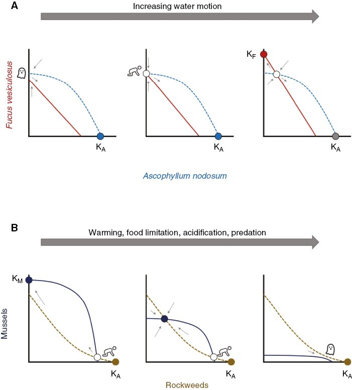
Models describing the transition between single stable and multiple stable states with changes in controlling parameters of environmental conditions. (A) Lotka–Volterra-like two species competition model showing variation of outcomes between Ascophyllum nodosum (dashed, blue line) and Fucus vesiculosus (solid, red line) in different hydrodynamic environments. Ka and Kf refer to the carrying capacities of A. nodosum and F. vesiculosus, respectively. On sheltered shores (top left), A. nodosum forms a single stable state (solid blue circle) with F. vesiculosus as a long-transient intermediate successional stage caused by a ghost attractor. With slightly increased water motion (top middle) leading to greater abundance of F. vesiculosus, the phase portrait contains an unstable equilibrium (open circle) with F. vesiculosus and a stable equilibrium with A. nodosum. The saddle associated with the unstable equilibrium results in F. vesiculosus being a long transient in the A. nodosum attractor caused by a ‘crawl-by’. On moderately exposed shores (top right), greater abundance of F. vesiculosus leads to alternative stable states of either F. vesiculosus (solid red circle) or A. nodosum and an unstable equilibrium of coexistence. (B) Lotka–Volterra-like two species competition model showing variation of outcomes between rockweeds (dashed, gold line) and mussels (solid, black line) under different environmental conditions on sheltered shores. Ka and Km refer to the carrying capacities of rockweeds (usually A. nodosum) and mussels, respectively. In cool, high pH, productive seawater (bottom left and middle) alternative stable states of mussels, rockweeds or a mix occur. With warming and acidification of seawater, less productivity and greater predation pressure also occur and the performance of mussels declines, shifting their isocline downward and annihilating both stable (solid black circle) and unstable (open circle) equilibria associated with mussels, leaving a ghost attractor and a single stable rockweed state (solid, gold circle).

Subtidal reefs of Port Phillip Bay, Australia

The first case study is from shallow subtidal reefs in Port Phillip Bay adjacent to the city of Melbourne and Australia’s largest urbanized embayment, which manifest at least three stable states as kelp beds (with Ecklonia radiata as the principal canopy-forming species), algal turf communities or sea urchin (Heliocidaris erythrogramma) barrens (Fig. 3). Different configurations in which fucoids or the invasive Asian kelp (Undaria pinnatifida) dominate the macroalgal community may represent further stable states, but more experimentation is required to determine this, so the account here will focus only on transitions between E. radiata-dominated kelp beds, turf assemblages and sea urchin barrens. Each of these configurations is maintained by strong positive feedbacks, and the mechanisms for transition from one state to another are well understood.

Manipulative experiments have demonstrated the urchin density at which destructive grazing of kelp occurs to form urchin barrens, and the density to which urchins much be reduced for the kelp to recover (Kriegisch et al., 2016, 2020), although increased availability of drift kelp will also reduce foraging on attached Ecklonia (Kriegisch et al., 2019a). Recruitment of the kelp is highest in dense kelp, where sweeping of the substratum by the Ecklonia blades and relatively low light levels prevents turf communities from establishing (Kriegisch et al., 2016; Reeves et al., 2018). These positive feedbacks to maintain Ecklonia beds and inhibit turf algae are also demonstrated at other locations in eastern and southern Australia (e.g. Kennelly, 1989; Gorman and Connell, 2009; Layton et al., 2019a). In this context it is interesting to note that Ecklonia beds provide a fluctuating chemical microenvironment that stimulates growth of juvenile Ecklonia (Britton et al., 2016).

Once urchin overgrazing removes the kelp, turf algae proliferate providing urchin density is not too high, and the resultant matrix of filamentous turf and semi-consolidated sediment inhibits kelp recruitment (Reeves et al., 2018; Kriegisch et al., 2019b), as has been observed for E. radiata beds elsewhere in south-east Australia (Kennelly, 1987; Valentine and Johnson, 2003, 2005; Gorman and Connell, 2009; Layton et al., 2020). Once it forms, urchin grazing is not required for the turf–sediment matrix to be maintained, and extensive turf cover devoid of any kelp but with zero or low numbers of urchins occur in some parts of the bay. The effect of a turf–sediment matrix inhibiting recruitment of larger macroalgae on shallow reefs is reported widely from around the world (see reviews by Strain et al., 2014; Filbee-Dexter and Wernberg, 2018), and may result from the particular light and chemistry of the turf microenvironment and/or lack of a solid substratum on which kelp gametophytes and microsporophytes can develop (Kennelly, 1987; Layton et al., 2019b). Moreover, it can be expected that availability of kelp spores is low over extensive areas of turf where the nearest kelp may be some distance away.

Where urchin grazing is sufficiently high in Port Phillip Bay, the urchins can maintain a ‘typical’ barrens configuration characterized by bare rock (Reeves et al., 2022).

Rocky shores of Maine, USA

Sheltered bays in Maine comprise habitats ranging from moderate to very low hydrodynamic exposure and large stretches of shoreline can be occupied by either of three different persistent community states: assemblages dominated by fucoid algae, either Ascophyllum nodosum – the most common state, stands of Fucus vesiculosus (collectively referred to as rockweeds), or beds of barnacles (Semibalanus balanoides) and mussels (Mytilus edulis and to a lesser extent in eastern Maine M. trossulus) (Petraitis et al., 2009; Dudgeon and Petraitis, 2019, 2022). Many common species are shared among these communities differing in abundances relative to one another among states.

The butterfly catastrophe model accommodates the complexity of experimental outcomes observed in sheltered bay habitats (Fig. 1D). Pulse perturbations to A. nodosum-dominated communities that mimicked ice scour clearing patches of rocky shore ranging in size from ~1 to 50 m² during winter 1997 resulted in large clearings switching to persistent communities of F. vesiculosus, or mussels and barnacles at the very same site. These outcomes meet the criterion of Peterson (1984) for alternative stable states. In contrast, small clearings mostly reverted to A. nodosum, and controls remained dominated by A. nodosum (Petraitis and Dudgeon, 2005; Petraitis et al., 2009). Transitions between states were enabled by greater recruitment and less consumption of F. vesiculosus, barnacles and mussels in large compared to small experimental clearings associated with reduced influence of consumers from the surrounding community on succession in large clearings. Additionally, recruitment and survivorship of A. nodosum were poor in large clearings (Petraitis and Dudgeon, 1999; Dudgeon and Petraitis, 2001, 2005; Petraitis et al., 2003). Recruitment data for rockweeds and mussels used as linear combinations of controlling parameters supported the bi-modal distribution of assigned states of either rockweed- or mussel-dominated communities to experimental plots (Petraitis and Dudgeon, 2015a).

A second pulse perturbation during winter 2011 to half of the originally cleared plots showed three important, and complex, outcomes (Dudgeon and Petraitis, 2022). First, large clearings showed variable outcomes with respect to the prior clearings; mussels, which have largely disappeared from the Gulf of Maine since 2010 (discussed below), did not recolonize and instead were replaced either by F. vesiculosus or A. nodosum. This suggests an important role for contingency, consistent with hypotheses of the origin of alternative stable states. Second, many stands of F. vesiculosus that quickly colonized and persisted for several generations in the original clearings were resilient to perturbation of their populations, consistent with the hypothesis of Fucus as a potential stable state in some sheltered bays, especially among sites with a greater range of water motion. However, in habitats that tend to have less water motion F. vesiculosus colonized slowly and was a long transient that was eventually replaced by A. nodosum after 15–18 years in small clearings, or after 23–25 years in large clearings.

The positive correlation between resilience of F. vesiculosus populations and water motion suggests that on moderately exposed to slightly sheltered shores, Fucus and A. nodosum represent alternative stable states determined by priority effects enabling either species to inhibit the other as implied by the phase portrait of the competition model with two stable equilibrium points and one unstable equilibrium point (Fig. 4A; Dudgeon and Petraitis, 2022). Recruitment, growth, survivorship and resilience of F. vesiculosus populations decline with water motion, and hence its zero-growth isocline crosses below that of A. nodosum leaving the former species as a long transient in a community dominated by the latter (Fig. 4A).

It is worth emphasizing that as parameters change, the equilibrium surface of the model changes, either wiggling due to variability in ecological processes or reshaping in response to environmental trends that affect relationships among species and their environment as the system moves towards a fold or cusp. Historically, communities of A. nodosum or beds of mussels and barnacles were the most frequent community states in sheltered bays. By 2010, mussel beds were in an accelerating decline throughout New England and now are relatively rare (Sorte et al., 2017; Commito et al., 2019; Petraitis and Dudgeon, 2020). Contemporaneously with the decline of mussels, warming and continued ocean acidification in the Gulf of Maine as well as eutrophication, habitat modification, invasions and range expansions, fishing and extreme events have directly and indirectly impacted coastal ecosystems. We suggest these changes have reshaped the rocky shore ecosystem in Maine from a system supporting one to three community states (i.e. butterfly catastrophe, Fig. 1D) to one that supports one or two states (i.e. cusp catastrophe, Fig. 1C) of fucoid algae and loss of the mussel-dominated community state. Present evidence suggests that alternative hypotheses causing the decline of mussels in the Gulf of Maine are warming, food availability and/or acidification affecting larval stages in the water column, and predation by non-native crabs on juveniles (Pechenik et al., 1990; Miller, 2013; Matassa and Trussell, 2015; Petraitis and Dudgeon, 2020). In the context of a phase portrait of a Lotka–Volterra-like competition model, these factors are hypothesized to change the position of the mussel isocline relative to fucoid algae from largely competitive dominance (left panel) to alternative stable states (middle panel) to dominance by fucoids (right panel; Fig. 4B).

USING CHARACTERISTIC LENGTH SCALES TO INDICATE PHASE SHIFT

Ecological systems are inherently ‘noisy’, i.e. some level of variability in time and space is ubiquitous. For species such as the giant kelp (Macrocystis pyrifera), inter-seasonal and inter-annual variability can be very large, dependent on storm patterns (Schiel and Foster, 2015). How then does an ecologist determine what is ‘normal’ variability and fluctuating dynamics within a single domain of attraction, and distinguish this from community change that represents some form of phase shift that demands a deft response from managers? It is clear that observing system state alone is insufficient to determine phase shift because there may be large and/or persistent transients within a single basin of attraction (see previous comments; also Scheffer and Carpenter, 2003; Scheffer et al., 2012).

The application of CLSs may offer an unambiguous means to detect phase shift in natural systems. The concept of the CLS was originally applied to ecology by Keeling et al. (1997) and Pascual and Levin (1999), and defines the optimal spatial scale at which to observe the deterministic dynamics of an ecosystem, i.e. where the signal to noise ratio is maximal. The CLS is a community-level property, and can be calculated from the spatio-temporal dynamics of any one species in a community of interacting species. The underlying tenet is that if the nature of the attractor of a system changes (i.e. there is a phase shift), then the CLS of that system will change. In other words, if there is a fundamental shift in the nature of underlying dynamics, then the optimum scale at which to most clearly observe those dynamics will also change; as the attractor changes, the capacity to predict the path of the attractor must also change at a given scale of observation (see below). Conversely, if community composition changes but there is no change in the CLS, this does not represent a phase shift. Transients such as these might arise, for example, when one or more haphazard forcing events push a system around in a single basin of attraction.

The theoretical approach of Keeling et al. (1997) and Pascual and Levin (1999) was applied to long time series of single species, and used time-delay embedding (Takens, 1981) to reconstruct the attractor for the entire system (or community). The time series was observed at a particular scale, or size of the window of observation on the system of interest. The position of the phase-space trajectory at time t + 1 was estimated from its position at time t and the movement of its k nearest neighbours in a single time step, assuming that neighbouring points on the reconstructed attractor have similar trajectories. The difference between the predicted and observed phase space trajectories determine the magnitude of the prediction error (a form of variance). This process is repeated for a large number of window sizes (i.e. across a range of scales of observation of the system), and a variance spectrum is produced by plotting the prediction error against scale (i.e. window size). The point of inflection in this curve where the spectrum begins to flatten out is defined as the CLS.

A key problem with the initial theoretical approach is that it required very long time series of highly spatially resolved data, which are not usually available for real ecosystems. However, Habeeb et al. (2005) showed that the data problem could be solved by substituting space for time, i.e. either by sliding ‘windows’ (i.e. quadrats) of different sizes around on a two-dimensional (2-D) map or ‘landscape’, or constructing the attractor piecemeal by considering a large number of windows (across a range of sizes) on a landscape over very few (e.g. two or three) times steps. Recognizing that sometimes even 2-D spatial data are not available for ecological systems, Ward et al. (2018) developed the approach further and showed that CLSs could be derived from 1-D spatial data, i.e. transect data. Transects are commonly used to provide descriptive data of marine systems, and widely used to quantify community structure in macroalgal systems.

This approach shows some promise. Johnson (2009) used spatial models to show that the CLS did not change for systems where community composition fluctuated massively around a single attractor (i.e. within a single basin of attraction), and that the CLS was agnostic to the single species chosen for observation and whether that chosen species tended to be rare or abundant at the time of observation. In contrast, if the dynamics of the system changed in a fundamental way (i.e. the position or shape of the attractor was changed) as a result of a shift in the environment that allowed, for example, proliferation of an invasive species, or which impacted relative growth rates, recruitment patterns or other facets of competitive ability, then the change in dynamics was reflected by a shift in the CLS.

When applied to a real ecological system (a highly biodiverse subtidal marine fouling community on a cave wall), the CLS calculated from any one of several taxonomically disparate interacting species was similar, as predicted by theory (Johnson et al., 2017). In this study, the single species examined that manifested a different CLS was one whose abundance was largely independent of other species on the wall, i.e. there was no evidence of strong interactions with other species in the system. Earlier work showed that length scales could also be measured from the spatial dynamics of different marine habitat types, and in this case was also insensitive to overall cover per se of a particular habitat type (Habeeb et al., 2007).

While these collective results are encouraging, the application of CLSs to assist with interpretation of changes in community structure and the detection of phase shift requires further testing. With the relatively recent advent of a method to estimate CLSs from transect data (Ward et al., 2018), there is the possibility of more widespread testing of the approach, particularly as applied to macroalgal-dominated systems. However, using length scales to detect a phase shift cannot differentiate between continuous and discontinuous shifts, which should be a critical question for managers. Options to determine the nature of a phase shift include conducting experiments to test for hysteresis (e.g. Kriegisch et al., 2016; although these kinds of experiments are conducted relatively rarely) or whether a pulse perturbation can cause a shift between states, and assessing the emergent dynamics of validated quantitative simulation models to determine the likelihood and characteristics of phase shift (Melbourne-Thomas et al., 2011; Marzloff et al., 2013). Overall, there would seem to be a long way to go yet in closing the gap between theoretical frameworks and real-world detection of phase shift (see review Andersen et al., 2008), particularly in applying detection methods that are not dependent only on system state.

QUANTIFYING ENVIRONMENTAL VARIABILITY TO ESTIMATE POTENTIAL FOR PHASE SHIFTS

One goal of ecology should be to provide tools facilitating effective, proactive management of ecosystems. Such an approach to management reduces the likelihood of ecological surprises, reactive responses in haste to restore an ecosystem and, hopefully, the incidence of large-scale changes that effect a loss of ecosystem services. A key strategy to proactive management should include quantitative estimates of vulnerability of an ecosystem to long transient stages or phase shifts under current, or projected, environmental conditions. We suggest the need to quantify metrics of environmental variability to estimate the potential of these kinds of changes.

This is not an easy task because it requires collecting a lot of data from both routine monitoring and experiments to characterize latent variables (i.e. resilience, thresholds and relative locus of the system) that are difficult to measure and accurately characterize (van Nes and Scheffer, 2007; Petraitis and Dudgeon, 2015b). Nevertheless, it is important because that characterization provides some estimate of the likelihood of change of state (extreme events notwithstanding) and, as importantly, defines the kind of evidence that can be expected and is relevant to addressing the nature of a hypothesized phase shift (i.e. expectation, or not, of EWS, hysteresis and divergence to occur; see above).

There are three important sources of variability to characterize: (1) noise in state variables, especially associated with extrinsic-environment-caused perturbation; (2) variability in parameters, which represent small ephemeral changes, or wiggling, of the potential surface of the basin of attraction; and (3) environmental trends that are known, or hypothesized, to have a correlative, or functional, relationship with parameter(s) hypothesized as drivers of phase shift dynamics. The latter two are depicted by horizontal movements of the system parallel to the environmental variables axes in each panel of Fig. 1, whereas noise in state variables from extrinsic perturbations are vertical vectors (parallel to the ordinate). Small changes in parameters that ‘wiggle the surface’ might also ‘jiggle the ball around’ such that the net vector summing vertical and horizontal movement represents noise in state variables.

The principal challenge is to estimate these variabilities relative to estimates of system resilience (i.e. as a proportion of distances to tipping points). One approach is time- and labour-intensive and involves combining collections of time series data from monitoring programmes or experiments with data from experiments to estimate resilience. The variable of interest in time series data is the standard deviation of variables from the collection of sampling units in space and time. Assuming that variance from observer error is negligible, the standard deviation of state variable(s) reflects their noise. It can be correlated with environmental time series data to identify anomalous observations as candidate natural perturbations. The variable of interest from an experiment perturbing state variables and measuring recovery time is resilience. A range of levels of perturbation allows estimation of resilience from small perturbations using the method of van Nes and Scheffer (2007), and potentially by direct observation by bracketing the tipping point (Petraitis and Dudgeon, 2004). In this way, the distribution over time of the state of the system (to the extent that the time period sampled is representative of the environment) can be compared relative to the estimate(s) of resilience to assess the probability of a phase shift by the proximity of the distribution tails to the tipping point. In addition to press experiments of a hypothesized controlling parameter(s) to test resilience (i.e. the domain of states from which the system can recover) and detect phase shift (e.g. Benedetti-Cecchi et al., 2015), experiments designed to estimate the variability of a controlling parameter estimate wiggling of the surface and its potential to push a system beyond a tipping point.

We suggest that another, simpler and less-labour intensive approach may be fruitful to characterize the variability of the ecosystem using CLSs. Given that CLS measures appear to be a means of reconstructing a basin of attraction, then (again, assuming negligible observation variance) the coefficient of variation calculated from repeated estimates of CLSs from the same ecosystem taken from different species at different times and locations in the same habitat directly capture ephemeral variability of the surface wiggling.

CONCLUSIONS

Many instances of large changes in the species composition of several different ecosystems has made phase shifts a familiar concept among ecologists. Despite widespread conceptual understanding of phase shifts, it nevertheless remains largely a ‘black box’ that is difficult to apply in a practical manner because of the lack of ‘fingerprint’ metrics to identify and distinguish phase shifts and which are easily quantifiable and uniquely characterize the signature of a community. We have reviewed the use of the CLS as a useful metric that uniquely identifies the basin of attraction of a community, thereby enabling distinction between phase shifts from long transients within a perturbed assemblage. Variabilities of CLSs and time series data may likewise provide metrics that shed light on the variabilities of state variables and parameters of natural ecosystems. Such metrics could be useful to managers to evaluate the propensity of a community to undergo phase shifts as a means of proactive, effective management to mitigate against potential phase shifts and the loss of ecosystem services.

FUNDING

Steve Dudgeon’s research is supported by the US National Science Foundation, grant numbers DEB-1020480 and DEB-1555641.

LITERATURE CITED

- Andersen T, Carstensen J, Hernandez-Garcia E, Duarte CM.. 2008. Ecological thresholds and regime shifts: approaches to identification. Trends in Ecology and Evolution 24: 49–57. [DOI] [PubMed] [Google Scholar]
- Andrew NL, Underwood AJ.. 1993. Density-dependent foraging in the sea urchin Centrostephanus rodgersii on shallow subtidal reefs in New South Wales, Australia. Marine Ecology Progress Series 99: 89–98. [Google Scholar]
- Arnol'd, VI. 1992. Catastrophe Theory, 3rd Edition. New York: Springer-Verlag. [Google Scholar]
- Beisner BE, Haydon DT, Cuddington K.. 2003. Alternative stable states in ecology. Frontiers in Ecology and the Environment 1: 376–382. [Google Scholar]
- Benedetti-Cecchi L, Tamburello L, Maggi E, Bulleri F.. 2015. Experimental perturbations modify the performance of early warning indicators of regime shift. Current Biology 25: 1867–1872. [DOI] [PubMed] [Google Scholar]
- Bennet S, Wernberg T, Harvey ES, Santana-Garcon J, Saunders BJ.. 2015. Tropical herbivores provide resilience to a climate-mediated phase shift on temperate reefs. Ecology Letters 18: 714–723. [DOI] [PubMed] [Google Scholar]
- Boerlijst M, Oudman T, de Roos AM.. 2013. Catastrophic collapse can occur without early warning: examples of silent catastrophes in structured ecological models. PLoS One 8: e62033. [DOI] [PMC free article] [PubMed] [Google Scholar]
- Boettiger C, Hastings A.. 2012. Quantifying limits to the detection of early warning for critical transitions. J Roy Soc. Interface 9: 2527–2539. [DOI] [PMC free article] [PubMed] [Google Scholar]
- Bossomaier T, Barnett L, Harré M, Lizier JT.. 2016. An introduction to transfer entropy. Berne: Springer. [Google Scholar]
- Britton D, Cornwall CE, Revill AT, Hurd CL, Johnson CR.. 2016. Ocean acidification reverses the positive effects of seawater pH fluctuations on growth and photosynthesis of the habitat-forming kelp, Ecklonia radiata. Scientific Reports 6: 26036. [DOI] [PMC free article] [PubMed] [Google Scholar]
- Carpenter SR, Brock WA, Cole JJ, Kitchell JF, Pace ML.. 2008. Leading indicators of trophic cascades. Ecology Letters 11: 128–138. [DOI] [PubMed] [Google Scholar]
- Carpenter SR, Cole JJ, Pace ML, et al. 2011. Early warnings of regime shifts: a whole-ecosystem experiment. Science 332: 1079–1082. [DOI] [PubMed] [Google Scholar]
- Clements CF, Ozgul A.. 2018. Indicators of transitions in biological systems. Ecology Letters 21: 905–919. [DOI] [PubMed] [Google Scholar]
- Cobb RC, Filipe JAN, Meentemeyer RK, Gilligan CA, Rizzo DM.. 2012. Ecosystem transformation by emerging infectious disease: loss of large tanoak from California forests. Journal of Ecology 100: 712–722. [Google Scholar]
- Commito JA, Jones BR, Jones MA, Winders SE, Como S.. 2019. After the fall: Legacy effects of biogenic structure on wind-generated ecosystem processes following mussel bed collapse. Diversity 11: 1, 11. https://doi:10.3390/d1101001134712100 [Google Scholar]
- Connell JH, Sousa WP.. 1983. On the evidence needed to judge ecological stability or persistence. American Naturalist 121: 789–824. [Google Scholar]
- Conversi A, Dakos V, Gårdmark A, et al. 2015. A holistic view of marine regime shifts. Philosophical Transactions of the Royal Society, Series B 370: 20130279. 10.1098/rstb.2013.0279 [DOI] [Google Scholar]
- Dakos V, Carpenter SR, Van Nes EH, Scheffer M.. 2015. Resilience indicators: prospects and limitations for early warnings of regime shifts. Philosophical Transactions of the Royal Society, Series B 370: 20130263. [Google Scholar]
- Dudgeon SR, Petraitis PS.. 2001. Scale-dependent recruitment and divergence of intertidal communities. Ecology 82: 991–1006. [Google Scholar]
- Dudgeon S, Petraitis PS.. 2005. First year demography of the foundation species, Ascophyllum nodosum, and its community implications. Oikos 109: 405–415. [Google Scholar]
- Dudgeon SR, Petraitis PS.. 2019. Rocky intertidal shores of the northwest atlantic ocean. In: Hawkins SJ, Firth LB, Bohn K, Williams GA. eds. Interactions in the marine benthos: a regional and habitat perspective. Systematics Association Series, Vol. 47, 61–89. Oxford: Oxford University Press. doi: 10.1017/9781108235792.005 [DOI] [Google Scholar]
- Dudgeon, SR, Petraitis PS.. 2022. Experimental evidence for resilience of rockweeds on rocky shores in the Gulf of Maine, USA. Limnology and Oceanography 67: S211–S223. [Google Scholar]
- Dudgeon SR, Aronson RB, Bruno JF, Precht WF.. 2010. Phase shifts and stable states on coral reefs. Marine Ecology Progress Series 413: 201–216. [Google Scholar]
- Duggins DO. 1981. Sea urchins and kelp: the effects of short term changes in urchin diet. Limnology and Oceanography 26: 391–394. [Google Scholar]
- Filbee-Dexter, K, Scheibling RE.. 2014. Sea urchin barrens as alternative stable states of collapsed kelp ecosystems. Marine Ecology Progress Series 495: 1–25. [Google Scholar]
- Filbee-Dexter K, Wernberg T.. 2018. Rise of turfs: a new battlefront for globally declining kelp forests. BioScience 68: 64–76. [Google Scholar]
- Filbee-Dexter K, Wernberg T, Grace SP, et al. 2020. Marine heatwaves and the collapse of marginal North Atlantic kelp forests. Scientific Reports 10: 13388. [DOI] [PMC free article] [PubMed] [Google Scholar]
- Francis TB, Abbott KC, Cuddington K, et al. 2021. Management implications of long transients in ecological systems. Nature Ecology and Evolution 5: 285–294. [DOI] [PubMed] [Google Scholar]
- Fung T, Seymour RM, Johnson CR.. 2011. Alternative stable states and phase shifts in coral reefs under anthropogenic stress. Ecology 92: 967–982. [DOI] [PubMed] [Google Scholar]
- Fung T, Seymour RN, Johnson CR.. 2013. Warning signals of regime shifts as intrinsic properties of endogenous dynamics. American Naturalist 182: 208–222. [DOI] [PubMed] [Google Scholar]
- Gilmore R. 1981. Catastrophe theory for scientists and engineers. New York: John Wiley & Sons. [Google Scholar]
- Gorman D, Connell SD.. 2009. Recovering subtidal forests in human-dominated landscapes. Journal of Applied Ecology 46: 1258–1265. [Google Scholar]
- Habeeb R, Trebilco J, Wotherspoon S, Johnson CR.. 2005. Determining natural scales of ecological systems. Ecological Monographs 75: 467–487. [Google Scholar]
- Habeeb RL, Johnson CR, Wotherspoon S, Mumby PJ.. 2007. Optimal scales to observe habitat dynamics: a coral reef example. Ecological Applications 17: 641–647. [DOI] [PubMed] [Google Scholar]
- Hare SR, Mantua NJ.. 2000. Empirical evidence for North Pacific regime shifts in 1977 and 1989. Progress in Oceanography 47: 103–145. [Google Scholar]
- Harrold C, Reed DC.. 1985. Food availability, sea urchin grazing, and kelp forest community structure. Ecology 66: 1160–1169. [Google Scholar]
- Hastings A, Wysham DB.. 2010. Regime shifts in ecological systems can occur with no warning. Ecology Letters 13: 464–472. [DOI] [PubMed] [Google Scholar]
- Hastings A, Abbott K, Cuddington K, et al. 2018. Transient phenomena in ecology. Science 361: eaat6412. [DOI] [PubMed] [Google Scholar]
- Hastings A, Abbott K, Cuddington K, et al. 2021. Effects of stochasticity on the length and behaviour of ecological transients. Journal of the Royal Society, Interface 18: 20210257. [DOI] [PMC free article] [PubMed] [Google Scholar]
- Hill NA, Blount C, Poore AGB, Worthington D, Steinberg PD.. 2003. Grazing effects of the sea urchin Centrostephanus rodgersii in two contrasting rocky reef habitats: effects of urchin density and its implications for the fishery. Marine and Freshwater Research 54: 691–700. [Google Scholar]
- Hughes TP. 1994. Catastrophes, phase-shifts, and large-scale degradation of a Caribbean coral reef. Science 265: 1547–1551. [DOI] [PubMed] [Google Scholar]
- Johnson CR. 2009. Natural length scales of ecological systems: applications at community and ecosystem levels. Ecology and Society 14: 7. [Google Scholar]
- Johnson CR, Mann KH.. 1982. Adaptations of Strongylocentrotus droebachiensis for survival on barren grounds in Nova Scotia. In: Bay T, Lawrence JM. eds. Echinoderms: proceedings of the international conference. Rotterdam: Balkema, 277–283. [Google Scholar]
- Johnson, CR, Banks, SC, Barrett, NS, et al. 2011. Climate change cascades: shifts in oceanography, species’ ranges and marine community dynamics in eastern Tasmania. Journal of Experimental Marine Biology and Ecology 400: 17–32. [Google Scholar]
- Johnson CR, Chabot RH, Marzloff MP, Wotherspoon S.. 2017. Knowing when (not) to attempt ecological restoration. Restoration Ecology 25: 140–147. [Google Scholar]
- Keeling M, Mezic I, Hendry R, Mcglade J, Rand D.. 1997. Characteristic length scales of spatial models in ecology via fluctuation analysis. Philosophical Transactions of the Royal Society of London, Series B 352: 1589–1601. [Google Scholar]
- Kennelly S. 1987. Inhibition of kelp recruitment by turfing algae and consequences for an Australian kelp community. Journal of Experimental Marine Biology and Ecology 112: 49–60. [Google Scholar]
- Kennelly SJ. 1989. Effects of kelp canopies on understory species due to shade and scour. Marine Ecology Progress Series 50: 215–224. [Google Scholar]
- Knowlton, N. 1992. Thresholds and multiple stable states in coral reef community dynamics. American Zoologist 32: 674–682. [Google Scholar]
- Kriegisch N, Reeves S, Johnson CR, Ling SD.. 2016. Phase-shift dynamics of sea urchin overgrazing on nutrified reefs. PLoS One 11: e0168333. [DOI] [PMC free article] [PubMed] [Google Scholar]
- Kriegisch N, Reeves S, Flukes EB, Johnson CR, Ling SD.. 2019a. Drift-kelp suppresses foraging movement of overgrazing sea urchins. Oecologia 190: 665–677. [DOI] [PubMed] [Google Scholar]
- Kriegisch N, Reeves SE, Johnson CR, Ling SD.. 2019b. Top-down sea urchin overgrazing overwhelms bottom-up stimulation of kelp beds despite sediment enhancement. Journal of Experimental Marine Biology and Ecology 514-515: 48–58. [Google Scholar]
- Kriegisch N, Reeves SE, Johnson CR, Ling SD.. 2020. Sea urchin control of macroalgal communities across a productivity gradient. Journal of Experimental Marine Biology and Ecology 527: 151248. [Google Scholar]
- Krumhansl KA, Okamoto D, Rassweiler A, et al. 2016. Global patterns of kelp forest change over the past half century. Proceedings of the National Academy of Sciences of the USA 113: 13785. [DOI] [PMC free article] [PubMed] [Google Scholar]
- Lawrence JM. 1975. On the relationships between marine plants and sea urchins. Oceanography Marine Biology Annual Review 13: 213–286. [Google Scholar]
- Layton C, Shelamoff V, Cameron MJ, Tatsumi M, Wright JT, Johnson CR.. 2019a. Resilience and stability of kelp forests: the importance of patch dynamics and environment-engineer feedbacks. PLoS One 14: e0210220. [DOI] [PMC free article] [PubMed] [Google Scholar]
- Layton C, Cameron MJ, Shelamoff V, et al. 2019b. Chemical microenvironments within macroalgal assemblages: Implications for the inhibition of kelp recruitment by turf algae. Limnology and Oceanography 64: 1600–1613. [Google Scholar]
- Layton C, Cameron MJ, Tatsumi M, Shelamoff V, Wright JT, Johnson CR.. 2020. Habitat fragmentation causes collapse of kelp recruitment. Marine Ecology Progress Series 648: 111–123. [Google Scholar]
- Lewontin RC. 1969. The meaning of stability. In: Woodwell GM, Smith HH. eds. Diversity and stability in ecological systems, Vol. 22. Upton, NY: Brookhaven National Laboratory, 13–24. [Google Scholar]
- Ling SD, Johnson CR, Frusher S, Ridgway K.. 2009. Overfishing reduces resilience of kelp beds to climate-driven catastrophic phase shift. Proceedings of the National Academy of Sciences of the USA 106: 22341–22345. [DOI] [PMC free article] [PubMed] [Google Scholar]
- Ling SD, Scheibling RE, Rassweiler A, et al. 2015. Global regime shift dynamics of catastrophic sea urchin overgrazing. Philosophical Transactions of the Royal Society of London, Series B 370: 20130269. [Google Scholar]
- Marzloff MP, Johnson CR, Little LR, Soulié J-C, Ling SD, Frusher SD.. 2013. Sensitivity analysis and pattern-oriented validation of TRITON, a model with alternative community states: Insights on temperate rocky reefs dynamics. Ecological Modelling 258: 16–32. [Google Scholar]
- Marzloff MP, Little LR, Johnson CR.. 2016. Building resilience against climate-driven shifts in a temperate reef system: Staying away from context-dependent ecological thresholds. Ecosystems 19: 1–15. [Google Scholar]
- Matassa CM, Trussell GC.. 2015. Effects of predation risk across a latitudinal temperature gradient. Oecologia 177: 775–784. [DOI] [PubMed] [Google Scholar]
- May RM. 1977. Thresholds and breakpoints in ecosystems with a multiplicity of stable states. Nature 269: 471–477. [Google Scholar]
- Melbourne-Thomas J, Johnson CR, Fung T, et al. 2011. Regional-scale scenario modeling for coral reefs: a decision support tool to inform management of a complex system. Ecological Applications 21: 1380–1398. [DOI] [PubMed] [Google Scholar]
- Miller LP. 2013. The effect of water temperature on drilling and ingestion rates of the dogwhelk Nucella lapillus feeding on Mytilus edulis mussels in the laboratory. Marine Biology 160: 1489–1496. [Google Scholar]
- Morozov A, Abbott K, Cuddington K, et al. 2020. Long transients in ecology: theory and applications. Physics of Life Reviews 32: 1–40. [DOI] [PubMed] [Google Scholar]
- Pascual M, Levin SA.. 1999. From individuals to population densities: searching for the intermediate scale of nontrivial determinism. Ecology 80: 2225–2236. [Google Scholar]
- Pawlik JR. 2011. The chemical ecology of sponges on Caribbean reefs: natural products shape natural systems. Bioscience 61: 888–898. [Google Scholar]
- Pechenik JA, Eyster LS, Widdows J, Bayne BL.. 1990. The influence of food concentration and temperature on growth and morphological differentiation of blue mussel Mytilus edulis L larvae. Journal of Experimental Marine Biology and Ecology 136: 47–64. [Google Scholar]
- Pedersen EJ, Koen-Alonso M, Tunney TD.. 2020. Detecting regime shifts in communities using estimated rates of change. ICES Journal of Marine Science 77: 1546–1555. [Google Scholar]
- Peterson CH. 1984. Does a rigorous criterion for environmental identity preclude the existence of multiple stable points? American Naturalist 124: 127–133. [Google Scholar]
- Petraitis, P., 2013. Multiple stable states in natural ecosystems. Oxford: Oxford University Press. [Google Scholar]
- Petraitis PS, Dudgeon SR.. 1999. Experimental evidence for the origin of alternative communities on rocky intertidal shores. Oikos 84: 239–245. [Google Scholar]
- Petraitis PS, Dudgeon SR.. 2004. Do alternate stable community states exist in the Gulf of Maine rocky intertidal zone? Comment. Ecology 85: 1160–1165. [Google Scholar]
- Petraitis PS, Dudgeon SR.. 2005. Divergent succession and implications for alternative states on rocky intertidal shores. Journal of Experimental Marine Biology and Ecology 326: 14–26. [Google Scholar]
- Petraitis PS, Dudgeon SR.. 2015a. Variation in recruitment and the establishment of alternative stable states. Ecology 96: 3186–3196. [DOI] [PubMed] [Google Scholar]
- Petraitis PS, Dudgeon SR.. 2015b. Cusps and butterflies: multiple stable states in marine systems as catastrophes. Marine and Freshwater Research 67: 37–46. [Google Scholar]
- Petraitis, PS, Dudgeon SR.. 2020. Declines over the last two decades of five key invertebrate species in the western North Atlantic. Communications Biology 3: 591–597. [DOI] [PMC free article] [PubMed] [Google Scholar]
- Petraitis PS, Rhile EC, Dudgeon SR.. 2003. Survivorship of juvenile barnacles and mussels: spatial dependence and the origin of alternative communities. Journal of Experimental Marine Biology and Ecology 293: 217–236. [Google Scholar]
- Petraitis PS, Methratta ET, Rhile EC, Vidargas NA, Dudgeon SR.. 2009. Experimental confirmation of multiple community states in a marine ecosystem. Oecologia 161: 139–148. [DOI] [PMC free article] [PubMed] [Google Scholar]
- Poston T, Stewart I.. 1978. Catastrophe theory and its applications. London: Pitman. [Google Scholar]
- Reeves SE, Kriegisch N, Johnson CR, Ling SD.. 2018. Reduced resistance to sediment-trapping turfs with decline of native kelp and establishment of an exotic kelp. Oecologia 188: 1239–1251. [DOI] [PubMed] [Google Scholar]
- Reeves S, Kriegisch N, Johnson CR, Ling S.. 2022. Kelp habitat fragmentation reduces resistance to overgrazing, invasion and collapse to turf dominance. Journal of Applied Ecology 59: 1619–1631. [Google Scholar]
- Rindi L, Dal Bello M, Benedetti-Cecchi L.. 2018. Experimental evidence of spatial signatures of approaching regime shifts in macroalgal canopies. Ecology 99: 1709–1715. [DOI] [PubMed] [Google Scholar]
- Scheffer M, Carpenter S.. 2003. Catastrophic regime shifts in ecosystems: linking theory to observation. Trends in Ecology and Evolution 18: 648–656. [Google Scholar]
- Scheffer M, Carpenter S, Foley JA, Folke C, Walker B.. 2001. Catastrophic shifts in ecosystems. Nature 413: 591–596. [DOI] [PubMed] [Google Scholar]
- Scheffer M, Bascompte J, Brock WA, et al. 2009. Early-warning signals for critical transitions. Nature 461: 53–59. [DOI] [PubMed] [Google Scholar]
- Scheffer M, Carpenter S, Lenton TM, et al. 2012. Anticipating critical transitions. Science 338: 344–348. [DOI] [PubMed] [Google Scholar]
- Schiel DR, Foster MS.. 2015. The biology and ecology of giant kelp forests. Los Angeles: University of California Press. [Google Scholar]
- Schröder A, Perrson L, DeRoos AM.. 2005. Direct experimental evidence for alternative stable states: a review. Oikos 110: 3–19. [Google Scholar]
- Smale DA, Wernberg T, Oliver ECJ, et al. 2019. Marine heatwaves threaten global biodiversity and the provision of ecosystem services. Nature Climate Change 9: 306–312. [Google Scholar]
- Smith KE, Burrow MT, Hobday AJ, et al. 2023. Biological impacts of marine heatwaves. Annual Review of Marine Sciences 15: 119–145. [DOI] [PubMed] [Google Scholar]
- Sorte CJB, Davison VE, Franklin MC, et al. 2017. Long-term declines in an intertidal foundation species parallel shifts in community composition. Global Change Biology 23: 341–352. [DOI] [PubMed] [Google Scholar]
- Strain EMA, Thompson RJ, Michelli F, Mancuso FP, Airlodi L.. 2014. Identifying the interacting roles of stressors in driving the global loss of canopy-forming to mat-forming algae in marine ecosystems. Global Change Biology 20: 3300–3312. [DOI] [PubMed] [Google Scholar]
- Takens, F. 1981. Detecting strange attractors in turbulence. In: Rand, D., and Young, L., eds. Dynamical systems and turbulence, Warwick 1980. Lecture notes in mathematics. New York, USA: Springer-Verlag, 366–381. [Google Scholar]
- Thom R. 1975. Structural stability and morphogenesis. New York: Benjamin Addison-Wesley. [Google Scholar]
- Valentine JP, Johnson CR.. 2003. Establishment of the introduced kelp Undaria pinnatifida in Tasmania depends on disturbance to native algal assemblages. Journal of Experimental Marine Biology and Ecology 295: 63–90. [Google Scholar]
- Valentine JP, Johnson CR.. 2005. Persistence of sea urchin (Heliocidaris erythrogramma) barrens on the east coast of Tasmania: Inhibition of macroalgal recovery in the absence of high densities of sea urchins. Botanica Marina 48: 106–115. [Google Scholar]
- van Nes EH, Scheffer M.. 2007. Slow recovery from perturbations as a generic indicator of a nearby catastrophic shift. American Naturalist 169: 738-747. American Naturalist 169: 660. [DOI] [PubMed] [Google Scholar]
- Ward DFL, Wotherspoon S, Melbourne-Thomas J, Haapkylä J, Johnson CR.. 2018. Detecting ecological regime shifts from transect data. Ecological Monographs 88: 694–715. [Google Scholar]
- Wernberg T. 2021. Marine heatwave drives collapse of kelp forests in Western Australia. In: Jackson, R.B., Canadell, J.G. eds. Ecosystem collapse and climate change. Ecological Studies-Analysis and Synthesis, Vol. 241. Heidelberg: Springer, 325–343. 10.1007/978-3-030-71330-0_12 [DOI] [Google Scholar]
- Wernberg T, Bennett S, Babcock RC, et al. 2016. Climate-driven regie shift of a temperate marine ecosystem. Science 353: 169–172. [DOI] [PubMed] [Google Scholar]
- Wouters N, Dakos V, Edwards M, Serafim MP, Valayer PJ, Cabral HN.. 2015. Evidencing a regime shift in the North Sea using early-warning signals as indicators of critical transitions. Estuarine, Coastal and Shelf Science 152: 65–72. [Google Scholar]
- Zeeman EC. 1976. Catastrophe theory. Scientific American 234: 65–83. [Google Scholar]