

Abstract
The main factor causing irreversible blindness is glaucoma. Early detection greatly reduces the risk of further vision loss. To address this problem, we developed a domain adaptation-based deep learning model called Glaucoma Domain Adaptation (GDA) based on 66,742 fundus photographs collected from 3272 eyes of 1636 subjects. GDA learns domain-invariant and domain-specific representations to extract both general and specific features. We also developed a progressive weighting mechanism to accurately transfer the source domain knowledge while mitigating the transfer of negative knowledge from the source to the target domain. We employed low-rank coding for aligning the source and target distributions. We trained GDA based on three different scenarios including eyes annotated as glaucoma due to 1) optic disc abnormalities regardless of visual field abnormalities, 2) optic disc or visual field abnormalities except ones that are glaucoma due to both optic disc and visual field abnormalities at the same time, and 3) visual field abnormalities regardless of optic disc abnormalities We then evaluate the generalizability of GDA based on two independent datasets. The AUCs of GDA in forecasting glaucoma based on the first, second, and third scenarios were 0.90, 0.88, and 0.80 and the Accuracies were 0.82, 0.78, and 0.72, respectively. The AUCs of GDA in diagnosing glaucoma based on the first, second, and third scenarios were 0.98, 0.96, and 0.93 and the Accuracies were 0.93, 0.91, and 0.88, respectively. The proposed GDA model achieved high performance and generalizability for forecasting and diagnosis of glaucoma disease from fundus photographs. GDA may augment glaucoma research and clinical practice in identifying patients with glaucoma and forecasting those who may develop glaucoma thus preventing future vision loss.
Keywords: Domain adaptation, deep learning, low-rank representation, glaucoma, forecasting, diagnosis
1. Introduction
Glaucoma disease is a leading cause of irreversible blindness worldwide [3]. Early detection is an effective approach to slow glaucoma and prevent subsequent vision loss [4]. However, detecting glaucoma requires extensive clinical examination and assessment of imaging and visual field tests. Fundus photography is a convenient and non-expensive technique for recording the status of the optic nerve head structure [5–8]. Although, detecting glaucoma from fundus images requires there is a considerable disagreement in diagnosis even among experienced glaucoma experts [4, 9]. Therefore, developing highly accurate, dependable, and low-cost automated models to detect glaucoma from fundus images is critical in ophthalmology.
Several deep convolutional neural network (CNN) models have been introduced to automatically identify various ocular diseases such as diabetic retinopathy, age-related macular degeneration, and glaucoma [10–13]. Deep CNN models typically require massive, annotated datasets for training. Additionally, using training and testing subsets with equivalent distributions is a pre-requisite for these models; otherwise the accuracy may be compromised [14]. Since data annotation is a challenging and labor-intensive task, particularly in the healthcare field, domain adaptation (DA) techniques may be used to deal with these situations in which limited numbers of annotated data exist. Also, in real-world applications, the training and testing samples may often be extracted from dissimilar sources (e.g., fundus photographs collected from subjects of different races in different countries) leading to different distributions. DA models can address such problems by transferring knowledge from training (source domain) to the testing (unlabeled target domain) to minimize the discrepancy between the source and target data distributions [15, 16].
We developed a novel, deep domain adaptation model, named Glaucoma Domain Adaptation (GDA), and applied it to three different ocular datasets: the Ocular Hypertension Treatment Study (OHTS) [17], ACRIMA [18], and RIM-ONE [19], for both glaucoma diagnosis and forecasting (prediction). Fundus images in the OHTS were collected from subjects in 22 different centers in the U.S. using different cameras, with considerable variability in image quality, resolution, and characteristics. ACRIMA and RIM-ONE are two publicly available datasets of fundus photographs with annotations that we used for externally validating our model. Although most of the studies of deep learning approaches have been focused on glaucoma screening or diagnosis, we assess the utility of our GDA model for both diagnosing as well as forecasting of glaucoma. We utilized low-rank coding and a weighted source classifier to improve the performance of GDA. Experimental results show the effectiveness of GDA for forecasting and diagnosis of glaucoma disease based on fundus photographs. Our contributions are summarized as follows:
Creation of a domain adaptation feature learning model via low-rank representation for forecasting and diagnosis of glaucoma disease.
Mitigation of negative knowledge transfer from the source to the target domain based on a progressive weighting module to improve the accuracy.
Evaluation of the performance of the proposed model for glaucoma forecasting and diagnosis and compared with state-of-the-art. We show that our model achieved the highest performance compared with numerous existing methods.
The rest of this paper is organized as follows. The related works are reviewed in Section 2. Section 3 introduces our proposed model. Experimental results are given in Section 4. Finally, Section 5 provides a conclusion for this paper.
2. Related Works
2.1. Glaucoma Forecasting and Diagnosis based on OHTS Study
Several studies have been performed for glaucoma diagnosis based on the OHTS dataset but there has been only one published study for forecasting glaucoma based on this dataset.
Thakur et al. [1] developed a CNN architecture based on MobileNetV2 for prediction and glaucoma detection using the OHTS dataset. They used 45,379 OHTS fundus photographs (after excluding ~20% of the images) and achieved AUCs of 0.77 and 0.88 for forecasting glaucoma 4–7 and 1–3 years before glaucoma onset, respectively. They obtained an AUC of ~ 0.95 for glaucoma diagnosis, which was defined on the basis of optic disc or visual field abnormalities.
Two additional studies have used the OHTS dataset for diagnosing glaucoma. Lin et. al. [20] introduced GlaucomaNet, an ensemble deep CNN glaucoma diagnosis model based on DenseNet-201 and ResNet-152 obtained an AUC of ~ 0.90 based on 37,339 fundus photographs from the OHTS dataset. For this study, glaucoma was also defined on the basis of optic disc or visual field abnormalities.
Another study based on 37,339 fundus photographs collected from the OHTS dataset conducted by Fan et. al. [2, 21], utilized a ResNet-50 model to identify glaucoma and obtained AUCs of 0.91, 0.88, and 0.86, respectively for three different definitions of glaucoma that were based 1) solely on optic disc abnormality, 2) a combination of optic disc or visual field abnormality, or 3) solely on visual field abnormalities.
2.2. Deep Domain Adaptation in Glaucoma Research
Machine learning methods used in medical image analysis generally suffer from domain shift problems caused by differences in distributions between source (reference data) and target (query data) domains. To address this problem, domain adaptation (DA) has recently received much attention [22].
Shen et al. [23] proposed a multitask deep learning framework, which utilized an adversarial discriminative domain adaptation approach along with landmark detection to create domain-invariant, interpretable fundus images. They also proposed a semi-supervised DA for image quality assessment, which enhanced the generalized performance between the source and target domains.
Kadambi et al. [24] introduced an adversarial domain adaptation model based on Wasserstein distance for detecting the optic disc-and-cup boundary on fundus images. They exploited the domain adaptation method with Wasserstein distance to calculate cup-to-disc ratio (used to determine glaucoma risk) in an unsupervised manner and calculated the clinical value in the diagnosis of glaucoma.
Xu et al. [25] introduced an unsupervised DA network, named the Minimizing-entropy and Fourier Domain Adaptation network (MeFDA), to decrease the discrepancy among the source and target domains. First, they performed an adversarial optimization method on predicted segmentation entropy maps to decrease the domain shift. Then, they applied direct entropy-minimization to the unlabeled target domain to enhance the validity of prediction segmentation maps. To improve the prediction consistency in the target domain, they augmented the target domain data via the Fourier transform by exchanging the low-frequency section in the target data with corresponding part of the source data.
Liu et al. [26] proposed a multi-scale collaborative adversarial domain adaptation method (CADA) to overcome the underlying domain shift problem for improving the performance of the glaucoma screening convention. They utilized a multi-scale input training manner to overcome the knowledge loss when applying pooling layers in the network and proposed the integration of low-level and high-level features to improve network learning. They applied the adversarial learning method at multiple layers of the network for learning the invariant features for both encoder and decoder phases, simultaneously.
Chen and Wang [27] proposed an unsupervised DA model, named Input and Output Space Unsupervised Domain Adaptation (IOSUDA), to decrease the efficiency degradation in joint optic disc (OD) and optic cup (OC) segmentation in glaucoma disease. Their framework extracts the common content features and the style features of each domain via image translation. They conducted adversarial learning to enhance the similarity of segmentation maps from different domains.
Lei et al. [28] introduced an unsupervised DA method which is based on the image synthesis and feature alignment (ISFA) approach, in order to segment OD and OC on fundus images for assessment of glaucoma disease. They utilized the GAN-based image synthesis strategy along with boundary information for OD and OC to create target-like query data, that can act as the intermediate latent space among source and target domains data, thereby decreasing the domain discrepancy problem.
Liu et al. [29] proposed an adversarial learning-based domain adaptation method (ECSD-Net) to simultaneously solve the joint optic disc and optic cup segmentation task as well as the glaucoma classification task on fundus images from different domains. They combined the efficientdet-D7 with a deep separable convolutional network and used an adversarial based structure to align the distribution between the source and target domains to overcome the domain discrepancy problem.
Haider et al. [30] proposed two networks, the separable linked segmentation network (SLS-Net) and the separable linked segmentation residual network (SLSR-Net), for accurate pixel-wise segmentation of the OC and OD in retinal fundus photographs. SLS-Net and SLSR-Net improve the OC and OD segmentation efficiency via minimization of the spatial information loss. SLSR-Net performs external residual connections for feature empowerment. Both proposed networks comprise a separable convolutional connection to reduce the cost of networks and improve computational efficiency.
Zhou et al. [31] proposed data augmentation-based domain adaptation feature alignment (DAFA) to enhance the out-of-distribution generalization of fundus images for glaucoma detection, which is based on the principle of feature mapping to learn the invariant features and to decrease the effect of data distribution shifts by using maximum mean discrepancy (MMD). They generated two sample views by data augmentation and performed feature alignment between augmented views via semantic representation alignment and latent feature recalibration.
ALGORITHM I.
Low-rank coding optimization procedure
| Input: , , , |
| Initialization: , , , , |
| Output: , , |
| while converted do |
| 1. Fix the other variables, update by solving (7) |
| 2. Fix the other variables, update by solving (8) |
| 3. Fix the other variables, update by solving (9) |
| 4. Update the multipliers and parameters: , |
| 5. Check the convergence conditions: , |
| end while |
3. OUR PROPOSED GDA MODEL
In this section, we introduce our proposed Glaucoma Domain Adaptation model (GDA) for glaucoma diagnosis and glaucoma forecasting. GDA includes three major structures: general and domain-specific feature extraction, low-rank coding learning, and source classifier loss weighting by considering low-rank loss. In the following, we will discuss these three structures.
3.1. General and Domain-Specific Feature Extraction
As illustrated in Fig. 1, we extract features in two steps. To extract general features between source and target domains, we apply a convolutional neural network (CNN) that projects data from original feature space to the common subspace. We then extract specific features between source and target domains. General features extracted from the common subspace are projected to the specific subspaces. The output of the domain-specific subnetwork has a Softmax classifier for the source domain. We use an entropy classification loss function as provided in (1).
Fig. 1.

Diagram of the GDA that includes a two-stage network for extracting general and domain-specific features. The distribution divergence between two domains is reduced via low-rank structure Z. The source classifier has been adapted on the target by weighting method. Domain adaptation between the data of the source domain and the target domain is performed by mapping the data from the original space with dimensions m to a common subspace with dimensions , so that each transferred target sample can be matched with a combination of source samples under low-rank and sparse constraints. The dimensions of low-rank representation coefficient matrix are .
Throughout the network, all (source domain) and (target domain) are first input to CNN model to extract general features , i.e., and , then the general extracted features are fed to to extract the domain-specific features, i.e., and . For simplicity, in the rest of this paper, we represent them as and .
| (1) |
Cross entropy loss is minimized based on the probability distribution output calculated by Softmax with the one-hot-encoded ground truth label . One-hot-encoded implies that in each column-vector only one element is 1 and the remaining are zeroes. Also, we use target domain-specific features to calculate target discriminator loss (2). The classifier trained on the source data is more likely to misclassify target samples that are close to the classification boundary. We thus applied L2 regularization for classifiers’ probabilistic output of target domain data as target discriminator loss to prevent overfitting and enhance the generalization performance of the model.
| (2) |
where represents the probabilistic output of the classifier for a given target domain sample .
3.2. Low-rank Coding Learning
Let’s represent the source domain with data samples and marginal distribution , and the target domain with data samples and marginal distribution . Domain adaptation is essentially a subgroup of transfer learning when (means that and/or while . The and are number of samples in the source and target domains, respectively. The is low-rank reconstruction matrix. The dimension of the low-rank space is indicated by . The is the noise matrix to decrease the effect of noise and negative knowledge. Low-rank optimization is as follows [32]:
| (3) |
where is the nuclear norm of a matrix [33]. To measure how each target sample is related to source samples, we utilize low-rank coding learning presented in (4) and use the low-rank loss to reduce the discrepancy between source and target domain distributions (ALGORITHM I). The low-rank reconstruction implies that each sample in the target domain can be reconstructed by almost a linear combination of related samples in the source domain, and therefore it can capture more common discriminative information across domains.
So, the low-rank constraint can be applied to coefficient matrix for having a block-wise structure [34]. By calculating low-rank loss, we extract the similarity level between each target sample against related source samples. In the following, we optimize the problem shown in (3). To performing that, we introduce a relaxing variable and change (3) to an equivalent equation as follows:
| (4) |
where is low-rank reconstruction matrix. is the noise matrix to decrease the effect of noise and unrelated knowledge. is the nuclear norm of a matrix. , , and can be optimized by Augmented Lagrange Multiplier (ALM) method [35]. It will be iteratively optimized by updating each variable while the other variables remain constant. The solution of (4) is obtained by minimizing the following function A.
| (5) |
where and are Lagrange multipliers and is a penalty parameter. The main steps of solving (5) are as follows. All steps have closed-form solutions.
-
Update Z: is updated by solving optimization (6).
(6) -
Update J: To update , the following need to be solved (8).
(8) The singular value decomposition of matrix is with considering singular value , we have which is .
-
Update E: is updated by iterating optimization (9).
(9) To solve the above problem, we could use the shrinkage operator:(10) Shrinkage operator [36] is defined as: .
- Multipliers Y1, Y2 and iteration step-size are updated by (11).
(11)
3.3. Weighting the Source Classifier Loss by Considering Low-rank Loss
We utilize a loss function, where a progressive weighting process [37] quantifies the transferability of knowledge so that the source classifier is accurately adapted to classify the target samples. We want to select source samples that are more related to each target sample and increase their contributions to the final model. To do this, we introduce a threshold, in which, if the low-rank loss is more than the threshold, the source classifier loss is weighted to enhance the classification accuracy. We assessed various thresholds such as {0.01, 0.05, 0.1, 0.2, 0.5, 0.8, 1}. The accuracy of GDA first increased and then decreased as threshold changed (as a bell-shaped curve). According to results, we observed a proper trade-off value of 0.1 that achieved the highest performance. This technique mitigates the negative transfer [37, 38], so the learner would not transfer unrelated knowledge from the source domain to the target domain. The weight in transferability weighting scheme is denoted by , which is calculated and normalized by (12). We multiply the weight with the source classifier .
| (12) |
| (13) |
where is the number of batch size and is the weight of each source samples. shows the probability that each sample belongs to the source domain. By weighing the source classifier loss, the ability of source discriminator to adapt on target samples is improved and the contribution of the irrelevant samples of the source domain in the final model is reduced. The total loss of our method includes sum of the weighted source classification loss , the source classification loss , the low-rank loss , and the target discriminator loss .
| (14) |
To mitigate the impact of the noisy activations in the early phases of training, rather than fixing the adaptation factors and , we used a progressive schedule to gradually increase factors from 0 to 1 as , and remains constant throughout the investigation [39]. The training of the network is performed by mini-batch stochastic gradient descent (SGD). The main procedure is summarized in ALGORITHM II. More specifically, via minimizing classification loss , the network was capable of classifying source domain data. More accurately, via weighting the source classifier loss , the network more accurately mitigated the negative transfer, so the learner would not transfer unrelated knowledge from the source domain to the target domain. Via minimizing low-rank loss , the network learned domain-invariant representations and further aligned domain distributions. Ultimately, via minimizing target discriminator loss , the network prevented overfitting and enhanced the generalization performance of the model.
4. EXPERIMENTS
4.1. Benchmark Datasets
We evaluated our model based on retinal fundus images collected from three different benchmark glaucoma datasets, including OHTS, ACRIMA, and RIM-ONE. In the OHTS study, we selected two subsets for glaucoma diagnosis and forecasting (prediction). Our results are described in the following subsections.
ALGORITHM II.
The Main Procedure of our method (gda)
| Input: , , |
| Initialization: , , , |
| Output: |
| For do |
| 1. Sample images from source domain |
| 2. Sample images from target domain |
| 3. Take source and target samples into general subspace |
| 4. Take source and target general features into domain-specific subspaces |
| 5. Take source domain-specific features into source domain-specific discriminator |
| 6. Use source and target domain-specific features to calculate low-rank loss |
| 7. Weigh the source classifier loss by considering low-rank loss |
| 8. Use target domain-specific features to calculate target discriminator loss |
| 9. Update total loss |
| end for |
4.1.1. The OHTS study
The OHTS study [17] was a prospective and multicenter investigation (22 different centers in the US) that sought to delay or prevent vision loss in ocular hypertensive patients. A total of 66,742 fundus photographs (58,779 single-stereo and 7,963 pair-stereo) from 3272 eyes of 1636 subjects were collected annually throughout the study (~16 years). All patients included in the study initially had both a normal-appearing optic disc and normal visual field at the baseline visit. Details of the OHTS dataset and the process for detecting glaucoma have been described in previous studies [40, 41].
In our research, we utilized OHTS fundus images to determine whether our proposed model can accurately identify glaucomatous eyes before and after glaucoma development (onset of the disease) based on three scenarios: 1) eyes labeled as glaucoma due to optic disc abnormalities regardless of visual field abnormalities, 2) eyes labeled as glaucoma due to optic disc or visual field abnormalities except ones that are glaucoma due to both OD and VF abnormalities at the same time, and 3) eyes labeled as glaucoma due to visual field abnormalities regardless of optic disc abnormalities. We excluded 7,963 pair-stereo images (two fundus photos on a single image) and utilized 58,779 single-stereo images for the experiments. We did not apply any further exclusion criteria to investigate whether the model could work based on real-world images collected under different conditions and settings. We generated two different subsets for glaucoma diagnosis (detection of glaucoma on or after disease onset) and glaucoma forecasting (prediction of glaucoma approximately 1–3 years before disease onset).
The first subset that was used for glaucoma diagnosis included 43,276 fundus images in which 39,385 were from normal eyes and the remaining 3891 images were from eyes with glaucoma (due to optic disc or visual field abnormalities). From 3891 fundus images corresponding to glaucomatous eyes, approximately 29% were labeled as glaucomatous due to optic disc abnormalities only (scenario 1), 22% due to visual field abnormalities only (scenario 3), and 51% due to either optic disc abnormalities only or visual field abnormalities only (scenario 2). Notably, 49% of eyes were glaucomatous due to both optic disc and visual field abnormalities that were not included in our downstream analysis (easiest group with typically more severe cases). The number of selected images for scenarios 1, 2, and 3 were 1128, 1984, and 856, respectively.
The second subset included 40,582 fundus images in which 39,385 fundus images were from normal eyes and 1197 fundus images were from eyes that converted to glaucoma after about 1 to 3 years, based on either optic disc or visual field abnormalities. We used this subset for glaucoma forecasting. The number of selected images for scenarios 1, 2, and 3 were 347, 610, and 263, respectively.
In our experiments, we randomly selected (at patient level) 70% of the data for the source domain and 30% of the data for the target domain [42].
4.1.2. ACRIMA
ACRIMA [18] is a publicly available dataset composed of 705 fundus images collected from 309 normal and 396 glaucomatous eyes. This dataset is part of the ACRIMA project and was obtained from normal and glaucomatous patients with their previous consent and in accordance with the ethical standards of Helsinki. We used ACRIMA as a target domain only in order to validate our model.
4.1.3. RIM-ONE
RIM-ONE [19] is another publicly available dataset that includes 159 stereo fundus images collected from 261 normal and 194 glaucomatous eyes. Three hospitals have contributed to developing this database: Hospital Clínico San Carlos, Hospital Universitario de Canarias, and Hospital Universitario Miguel Servet. In our experiments, we also used this dataset as target domain only.
4.2. Implementation Details
Since training deep CNN models typically requires large training data, we employed a CNN architecture that was pretrained on ImageNet 2012 previously [43]. Our model automatically crops and resizes all images to 224×224×3. The OHTS dataset has an imbalanced number of images in each class, where approximately only 12% of the fundus photographs belong to eyes with glaucoma. To address this problem, we performed data augmentation via random rotations, vertical and horizontal flips, and randomly changed the saturation, hue, and contrast in the training fundus images. After augmentation, during model training, the same number of images were selected from each class in each batch. The coding was performed in Python based on the Pytorch, and all convolutional and pooling layers were fine-tuned based on Pytorch-provided models of ResNet50 [45]. The classifier was trained based on backpropagation. The optimization approach was mini-batch stochastic gradient descent (SGD) with momentum of 0.9 and learning rate where was selected from [0–1] range, , , and . The batch size for minibatch was 8 and the iteration was 250. We trained our model on a GPU machine with Nvidia GeForce RTX 3070.
To estimate the reliability of our proposed model, in the training phase, we split the target domain through a stratified 10-fold cross-validation strategy, whereas we kept one single fold aside for testing and fed the remaining nine folds (without their labels) as unlabeled target domain (along with source domain) into the model. We repeated the training and testing for each fold and then computed the average accuracies as final results.
4.3. Experimental Results
4.3.1. Glaucoma diagnosis on OHTS dataset
Table 1 presents AUCs, sensitivities, and specificities based on different scenarios for glaucoma diagnosis on the OHTS dataset.
Table 1.
Performance of the model for glaucoma diagnosis in terms of AUC, Sensitivity, and Specificity, based on three different scenarios: eyes Labeled as glaucoma due to “only optic disc abnormalities”, “optic disc or visual field abnormalities”, and “only visual field abnormalities” (presented as scenario 1, 2, and 3, respectively). P-values identified based on the method of DeLong. The significance level is p-value < 0.05
| Characteristics | AUC (95% CI) | Sensitivity (95% CI) | Specificity (95% CI) | DeLong P-value |
|---|---|---|---|---|
| Scenario 1 | 0.98 (0.96 −0.99) | 0.96 (0.94–0.98) | 0.90 (0.88–0.92) | Scenario 1~ Scenario 2: P= 0.24 |
| Scenario 2 | 0.96 (0.94–0.98) | 0.94 (0.91–0.96) | 0.87 (0.84–0.90) | Scenario 1~ Scenario 3: P= 0.03 |
| Scenario 3 | 0.93 (0.90–0.95) | 0.91 (0.88–0.93) | 0.85 (0.82–0.88) | Scenario 2~ Scenario 3: P= 0.12 |
Glaucoma is typically defined based on the abnormalities in either optic disc or visual field (scenario 2). However, we tested two other scenarios to assess the robustness of our model. As expected, the AUC of the model based on optic disc abnormalities only was significantly better than the AUC of the model based on visual field abnormalities only.
This finding was not unexpected because glaucoma experts report similar findings. Both our model and glaucoma experts appear to more readily identify optic disc abnormality manifested in fundus photographs, compared to identification of abnormalities manifested in visual fields only.
We also evaluated the performance of GDA using area under the receiver operating characteristic curve (AUC) and confusion matrix (Fig. 2). The results showed that the best diagnostic AUC and Accuracy rates were achieved for glaucoma detection based on the first scenario that glaucoma was defined based on the optic disc only (AUC = 0.98, Acc = 0.93); followed by the second scenario that glaucoma was defined based on either optic disc or visual field abnormalities (AUC = 0.96, Acc = 0.91), and lastly, the third scenario that glaucoma was defined based on visual field abnormality only (AUC = 0.93, Acc = 0.88).
Fig. 2.

ROCs and confusion matrices for three scenarios of glaucoma detection. (a) AUCs results of the proposed model for glaucoma detection based on “only optic disc abnormalities”, “optic disc or visual field abnormalities”, and “only visual field abnormalities” were 0.98 (0.96–0.99), 0.96 (0.94–0.98), and 0.93 (0.90–0.95), respectively. (b) the accuracy of glaucoma detection based on only optic disc abnormalities was 0.93, (c) accuracy of glaucoma detection based on optic disc or visual field abnormalities was 0.91, (d) accuracy of glaucoma detection based on only visual field abnormalities was 0.88.
Fig. 2 (a–d) shows the ROC curves and the confusion matrices corresponding to these different scenarios.
Fig. 3 (a–d) show class activation maps (CAMs) representing regions that were more important for the model to make the correct diagnosis. CAMs provide a means to evaluate the clinical relevance of the model. Based on the CAMs, it appears that the model is focused more on the optic disc and peripapillary region, mostly in the inferior hemifield of the retina, which are clinically meaningful, as clinicians also typically evaluate these regions to identify glaucoma.
Fig. 3.

Class activation maps (CAMs) represent regions that were more important for the model to make diagnosis. From left to right (a-d), CAMs correspond to a normal eye, eyes with glaucoma due to only optic disc abnormalities, optic disc or visual field abnormalities, and only visual field abnormalities, respectively.
4.3.2. Glaucoma forecasting based on the OHTS dataset
For glaucoma forecasting, we evaluated the performance of GDA using AUC, specificity, sensitivity, and accuracy on the OHTS dataset based on three different scenarios: 1) optic disc abnormalities regardless of visual field abnormalities, 2) optic disc or visual field abnormalities except ones that are glaucoma due to both optic disc and visual field abnormalities at the same time, and 3) visual field abnormalities regardless of optic disc abnormalities.
Table 2 presents AUCs of the GDA model based on different scenarios for glaucoma forecasting based on the OHTS dataset. As expected, the results showed that the best prediction AUC and Accuracy rates were achieved for glaucoma prediction based on the on the first scenario (glaucoma related to optic disc only) (AUC = 0.90, Acc = 0.82) followed by the glaucoma prediction model based on the on the second scenario (glaucoma related to either optic disc or visual field abnormalities) (AUC = 0.88, Acc = 0.78), then the third scenario (glaucoma related to visual field abnormalities only) (AUC = 0.80, Acc = 0.72). Fig. 4 (a–d) show the ROC curves and the confusion matrices corresponding to these different scenarios.
Table 2.
Performance of the model for glaucoma prediction in terms of AUC, Sensitivity, and Specificity, based on three different scenarios: eyes Labeled as glaucoma due to “only optic disc abnormalities”, “optic disc or visual field abnormalities”, and “only visual field abnormalities” (presented as scenario 1, 2, and 3, respectively). P-values identified Based on the method of DeLong. The Significance level is p-value < 0.05
| Characteristics | AUC (95% CI) | Sensitivity (95% CI) | Specificity (95% CI) | DeLong P-value |
|---|---|---|---|---|
| Scenario 1 | 0.90 (0.87 −0.92) | 0.83 (0.80–0.86) | 0.76 (0.73–0.77) | Scenario 1~ Scenario 2: P= 0.32 |
| Scenario 2 | 0.88 (0.85–0.90) | 0.80 (0.77–0.83) | 0.73 (0.70–0.75) | Scenario 1~ Scenario 3: P= 0.01 |
| Scenario 3 | 0.80 (0.77–0.82) | 0.72 (0.70–0.95) | 0.64 (0.61–0.66) | Scenario 2~ Scenario 3: P= 0.04 |
Fig. 4.

ROCs and confusion matrices for three scenarios of glaucoma prediction. (a) AUCs results of the proposed model for glaucoma prediction based on “only optic disc abnormalities”, “optic disc or visual field abnormalities”, and “only visual field abnormalities” were 0.90 (0.87–0.92), 0.88 (0.85–0.90), and 0.80 (0.77–0.82), respectively. (b) the accuracy of glaucoma prediction based on only optic disc abnormalities was 0.82, (c) accuracy of glaucoma detection based on optic disc or visual field abnormalities was 0.78, (d) accuracy of glaucoma detection based on only visual field abnormalities was 0.72.
4.3.3. Comparison with other methods on OHTS dataset
We compared our proposed model with other related methods that also used the OHTS as a benchmark. Thakur et. al. [1] developed a deep CNN model to diagnose and forecast glaucoma based on OHTS fundus images. They obtained AUCs of 0.97 for diagnosis of solely on optic disc abnormality and 0.88 for diagnosis of solely on visual field abnormality. However, they excluded about 20% of the images they deemed ungradable from the total dataset and tested their model on the 15% of the data. In comparison, we only excluded a few percent of the irrelevant images (those with a pair of stereo photos on a single retinal image) and included images with lower qualities and tested our GDA model based on 30% of randomly selected data, and yet were able to obtain slightly better diagnosis and forecasting accuracies. In both models, the testing subsets were selected based on the subject level rather than the eye level to avoid bias. In eye-level analysis, each eye of a patient is analyzed individually however both eyes of the same subjects are typically highly similar thus each eye may carry information from the other eye thus making the learning process biased if two eyes are placed in training and testing subsets. However, all metrics are then calculated at the eye level.
In comparison with another study conducted by Fan et. al. [2], our model obtained significantly higher AUCs with a 7% improvement based on two scenarios for diagnosis of solely on optic disc abnormality and for diagnosis of solely on visual field abnormality. They performed their training at the subject level and selected 20% of data for testing dataset. Table 3 shows the comparison results.
Table 3.
Comparison with other methods on OHTS dataset
4.3.4. Independent validation of the model based on publicly available datasets
To assure generalizability, we evaluated the performance of our model based on ACRIMA and RIM-ONE datasets (Table 4). In this experiment, we selected the OHTS diagnostic subset as the source and each of the ACRIMA and RIM-ONE datasets as the target domain. The AUCs of our model for detecting glaucoma based on ACRIMA and RIM-ONE datasets were 0.87 and 0.92, respectively (see Fig 5). Findings confirm a reasonably high degree of generalizability reflecting the fact that the model is robust and likely generalizable to unseen datasets.
Table 4.
Performance of the model for glaucoma diagnosis in terms of AUC, Sensitivity, and specificity, when OHTS (Scenario 2) is considered as Source domain and ACRIMA and RIM-ONE are considered as target domain
| Source dataset | Target dataset | AUC (95% CI) | Sensitivity | Specificity |
|---|---|---|---|---|
| OHTS (Scenario 2) | ACRIMA | 0.87 (0.83–0.90) | 0.85 (0.82–0.88) | 0.65 (0.62–0.68) |
| OHTS (Scenario 2) | RIM-ONE | 0.92 (0.89–0.95) | 0.89 (0.86–0.92) | 0.75 (0.72–0.78) |
Fig. 5.

ROCs for scenario 2 of glaucoma detection when the OHTS dataset is as the source domain and each of ACRIMA and RIM-ONE datasets are as the target domain.
4.4. Impact of demographic and ocular parameters on GDA
To investigate whether the GDA model is biased towards gender, age, race, MD, or IOP factors, we performed several supplemental and statistical analyses. We used the Delong’s test [44] for comparing the AUCs of the models and utilized a two-sided p-values of <0.05 for reporting statistical significance. As both eyes may be used in different subsets, we used Generalized Estimating Equation (GEE) to compare those characteristics of the eyes and accounted for both eyes of same subjects in statistical comparisons [45].
We then computed the AUCs of the models based on different genders and races, and different age, MD and IOP ranges. Table 5 shows the AUC of the GDA model based on these factors. As can be seen, the GDA model is not biased to any gender or race. Also, it is not biased towards age or IOP. However, the model was significantly more accurate in detecting those at the later stages of glaucoma (MD < −8 dB) compared to those at the early stages of glaucoma. This is, however, expected as glaucoma is more manifest in those at the later stages of the disease compared to those at the early stages of the disease. As such, the model is robust yet unbiased to demographic factors.
Table 5.
Performance of the model for glaucoma diagnosis in terms of AUC, Sensitivity, and Specificity, based on different genders, ages, races, glaucoma severity levels, and IOP. P-values were calculated based on the GEE model. The significance level is < 0.05
| Characteristics | AUC (95% CI) | Sensitivity | Specificity | GEE P-value |
|---|---|---|---|---|
| Gender | 0.46 | |||
| Female | 0.96 (0.94–0.98) | 0.94 (0.92–0.96) | 0.86 (0.84–0.89) | |
| Male | 0.95 (0.93–0.98) | 0.93 (0.91–0.96) | 0.85 (0.83–0.88) | |
| Age | 0.41 | |||
| < 55 years | 0.95 (0.92–0.97) | 0.93 (0.90–0.96) | 0.86 (0.83–0.90) | |
| ≥ 55 years | 0.96 (0.94–0.98) | 0.95 (0.93–0.97) | 0.87 (0.85–0.90) | |
| Race | 0.44 | |||
| Non African-American | 0.95 (0.92–0.97) | 0.93 (0.90–0.96) | 0.85 (0.82–0.88) | |
| African-American | 0.96 (0.93–0.98) | 0.94 (0.90–0.97) | 0.87 (0.84–0.90) | |
| Mean deviation (MD) | ||||
| ≥ 0 dB | 0.94 (0.91–0.96) | 0.89 (0.85–0.93) | 0.82 (0.78–0.86) | mild vs early:0.48 |
| −4 dB ≤ & < 0 dB | 0.95 (0.92–0.97) | 0.92 (0.89–0.95) | 0.84 (0.81–0.87) | moderate vs early: 0.27 |
| −8 dB ≤ & < −4 dB | 0.95 (0.93–0.97) | 0.93 (0.90–0.96) | 0.85 (0.83–0.88) | |
| ≤ −8 dB | 0.97 (0.94–0.99) | 0.95 (0.93–0.98) | 0.87 (0.85–0.90) | advanced vs early: 0.04 |
| Intraocular pressure (IOP) | 0.38 | |||
| < 21 mmHg | 0.95 (0.92–0.97) | 0.91 (0.89–0.94) | 0.85 (0.82–0.88) | |
| ≥ 21 mmHg | 0.96 (0.93–0.99) | 0.93 (0.90–0.96) | 0.88 (0.85–0.90) |
4.5. Justification of findings and clinical validation
While the accuracy of the GDA model was reasonably high, some fundus images were nevertheless misclassified. To identify the reasons for error, we analyzed some of the images that were misclassified. Most of the misclassified eyes in our model were labeled as glaucoma due to abnormalities in visual field only without any obvious sign of glaucomatous optic neuropathy (GON) manifested in fundus images. This can be justified as glaucoma was not identified in such eyes based on clinical evaluations performed by the OHTS imaging reading center as well and they labeled those eyes as glaucoma due to visual field abnormalities only. Additionally, some other misclassified fundus images were of poor quality, including those OHTS images that were scanned from analog fundus photographs. As a result, OHTS represents a dataset with overall low quality. Even so, we did not exclude any fundus photographs due to poor image quality. The results suggest that our novel architecture is more accurate and robust compared to previously developed models.
In a separate experiment, we compared the performance of the GDA model to a human expert. We randomly selected 100 fundus images from the OHTS dataset and compared the diagnostic accuracy of GDA against the diagnostic accuracy of a second-year ophthalmology resident. The diagnosis accuracy of the ophthalmology resident was 79% which was significantly lower than 88% accuracy of the GDA model.
4.6. Ablation Study
As GDA is composed of four loss functions that together minimize the ultimate misclassification error, we performed an ablation study to investigate the influence of each loss function on the GDA performance. Fig. 6 and Fig. 7 show the AUCs of the GDA model based on different ablation studies corresponding to the diagnosis or forecasting tasks. In each scenario, we performed three different ablation studies. Using: 1) baseline structure with and ; 2) baseline structure with and and ; and 3) baseline structure with and and and . The baseline structure represents a deep NN based on the ResNet50 architecture. When we added two sub deep networks for extracting general (G) and domain-specific (F) features along with and to the baseline structure, we obtained AUCs of 0.90, 0.86, and 0.84 based on scenarios 1, 2, and 3 for glaucoma diagnosis, and AUCs of 0.79, 0.76, and 0.71 based on scenarios 1, 2, and 3 for glaucoma forecasting, respectively. By adding the capability of domains alignment and decrease domain discrepancy through , we obtained improved AUCs of 0.95, 0.93, and 0.91 based on scenarios 1, 2, and 3 for glaucoma diagnosis, and improved ACUs of 0.86, 0.84, and 0.76 based on scenarios 1, 2, and 3 for glaucoma forecasting, respectively. Finally, by adding to the previous structure, it forces the source classifier to adapt further to the target samples thus improves the accuracy. In other words, the source samples with more similarity to the target samples are selected and their contributions are boosted in the final model. We obtained improved AUCs of 0.98, 0.96, and 0.93 based on scenarios 1, 2, and 3 for glaucoma diagnosis, and improved AUCs of 0.90, 0.88, and 0.80 based on scenarios 1, 2, and 3 for glaucoma prediction, respectively. As can be seen, the results support our initial idea of integrating these loss functions to improve the robustness and enhance the accuracy of the GDA model.
Fig. 6.

Ablation study based on three glaucoma diagnosis scenarios : AI baseline structure with cross entropy loss and target discriminator loss functions; : AI baseline structure with cross entropy, target discriminator loss, and low-rank loss functions; and : AI baseline structure with cross entropy, targe discriminator loss, low-rank, and weighting loss functions.
Fig. 7.
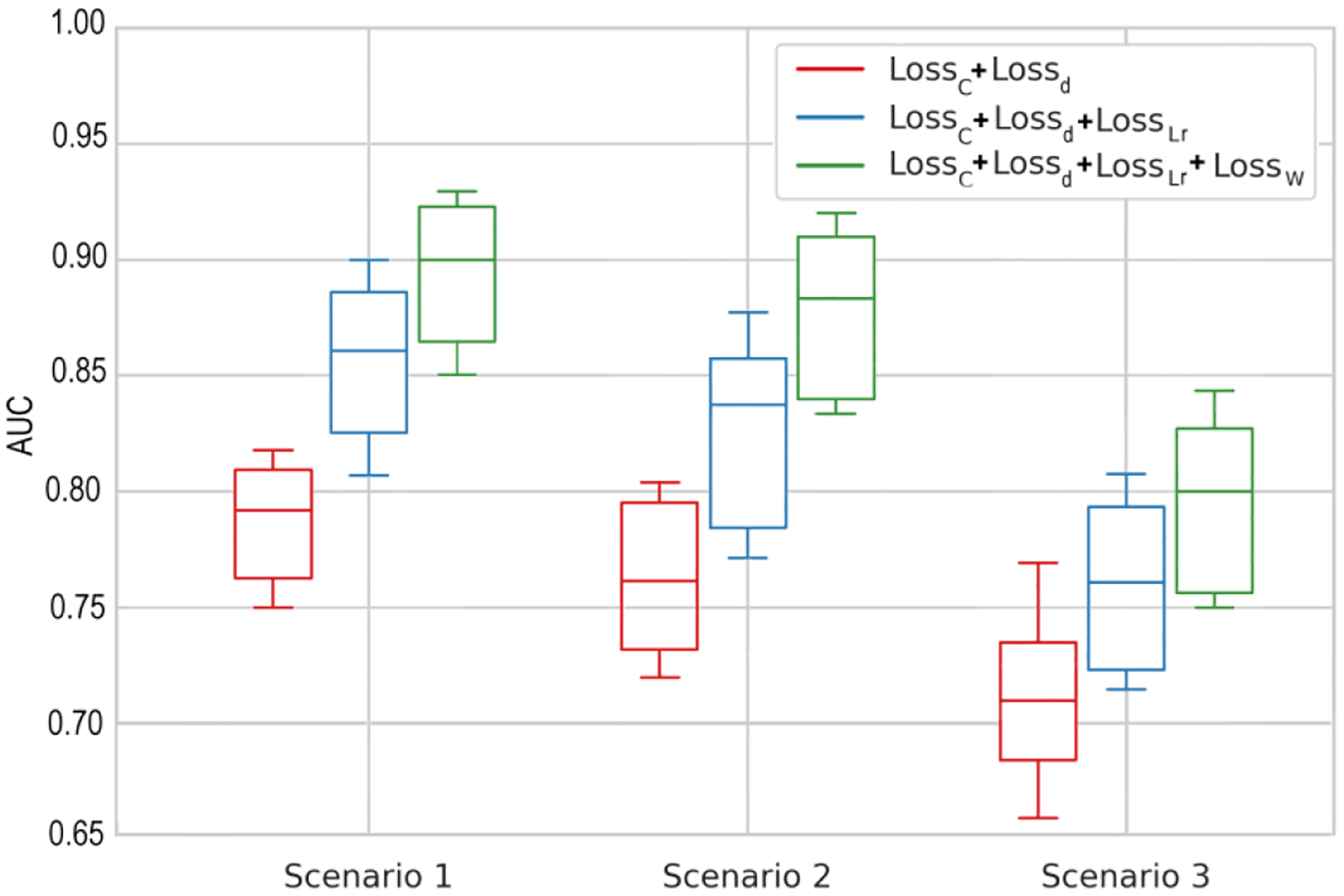
Ablation study based on three glaucoma forecasting scenarios. : AI baseline structure with cross entropy loss and targe discriminator loss functions; : AI baseline structure with cross entropy, target discriminator loss, and low-rank loss functions; and : AI baseline structure with cross entropy, target discriminator loss, low-rank, and weighting loss functions.
Further, we calculated the computational complexity for different structures of GDA. We ran each part of our model on a GPU machine with Nvidia GeForce RTX 3070 and recorded the average time of each iteration over 250 iterations. The results were as follows: 1) baseline structure with and (0.276 s); 2) baseline structure with and and (0.298 s); and 3) baseline structure with and and and (0.341 s). Comparing different structures showed that with compromising the computational complexity slightly, the accuracy improved significantly.
5. CONCLUSION
We introduced a novel deep domain adaptation model for diagnosis and forecasting of glaucoma from fundus photographs. The proposed model called GDA includes general and domain specific CNNs and a weighted source classifier to improve accuracy. Domain discrepancy between the source and target domains is minimized using low-rank coding. Experimental results based on three major independent glaucoma datasets showed a high diagnostic accuracy and generalizability. This method may augment glaucoma research and clinical practice by identifying patients with glaucoma and forecasting glaucoma development more accurately.
Like other CNN models, our proposed model can deal with images better than visual fields. Therefore, as expected, our model was more accurate based on fundus images with manifestation of glaucoma due to glaucomatous optic neuropathy compared to glaucoma due to manifestation of visual field abnormalities. Future studies may combine these models with other AI models that can exploit demographic, clinical, ocular, or visual field parameters.
Aacknowledgement
This work was supported by the National Institutes of Health [grant numbers EY033005, EY031725] and support from the Research to Prevent Blindness (RPB), New York. The funders had no role in study design, data collection and analysis, decision to publish, or preparation of the manuscript.
Footnotes
Publisher's Disclaimer: This is a PDF file of an unedited manuscript that has been accepted for publication. As a service to our customers we are providing this early version of the manuscript. The manuscript will undergo copyediting, typesetting, and review of the resulting proof before it is published in its final form. Please note that during the production process errors may be discovered which could affect the content, and all legal disclaimers that apply to the journal pertain.
CRediT authorship contribution statement
Yeganeh Madadi: Conceptualization, Methodology, Software, Data curation, Writing – original draft, Visualization, Investigation. Hashem Abu-Serhan: Clinical validation. Siamak Yousefi: Supervision, Data curation, Validation, Writing – review & editing.
Declaration of Competing Interest
Siamak Yousefi has acted as a consultant for EnoLink and is an equity owner in InsightEye LLC. He has received prototype instruments from Remidiom M&S Technologies, and Virtual Fields. Other authors declare that they have no known competing financial interests or personal relationships that could have appeared to influence the work reported in this paper.
Data availability
Data is available on https://github.com/DM2LL/GDA.
References
- [1].Thakur A, Goldbaum M, and Yousefi S, “Predicting Glaucoma before Onset Using Deep Learning,” Ophthalmol Glaucoma, vol. 3, no. 4, pp. 262–268, Jul – Aug 2020, doi: 10.1016/j.ogla.2020.04.012. [DOI] [PMC free article] [PubMed] [Google Scholar]
- [2].B. C Fan Rui, Christopher Mark, Brye Nicole, Proudfoot James A., Jasmin, et al. , “Detecting Glaucoma in the Ocular Hypertension Study using deep learning,” JAMA Ophthalmol, vol. 140, no. 4, pp. 383–391, 2022, doi: 10.1001/jamaophthalmol.2022.0244. [DOI] [PMC free article] [PubMed] [Google Scholar]
- [3].Zhang N, Wang J, Li Y, and Jiang B, “Prevalence of primary open angle glaucoma in the last 20 years: a meta-analysis and systematic review,” Sci Rep, vol. 11, no. 1, p. 13762, Jul 2 2021, doi: 10.1038/s41598-021-92971-w. [DOI] [PMC free article] [PubMed] [Google Scholar]
- [4].Kolomeyer NN et al. , “Lessons Learned From 2 Large Community-based Glaucoma Screening Studies,” Journal of Glaucoma, vol. 30, no. 10, pp. 875–877, 2021. [DOI] [PMC free article] [PubMed] [Google Scholar]
- [5].Iqbal S, Khan TM, Naveed K, Naqvi SS, and Nawaz SJ, “Recent trends and advances in fundus image analysis: A review,” Comput Biol Med, vol. 151, no. Pt A, p. 106277, Dec 2022, doi: 10.1016/j.compbiomed.2022.106277. [DOI] [PubMed] [Google Scholar]
- [6].Bhati A, Gour N, Khanna P, and Ojha A, “Discriminative kernel convolution network for multi-label ophthalmic disease detection on imbalanced fundus image dataset,” Comput Biol Med, vol. 153, p. 106519, Feb 2023, doi: 10.1016/j.compbiomed.2022.106519. [DOI] [PubMed] [Google Scholar]
- [7].Nawaldgi S and Lalitha YS, “Automated glaucoma assessment from color fundus images using structural and texture features,” Biomedical Signal Processing and Control, vol. 77, 2022, doi: 10.1016/j.bspc.2022.103875. [DOI] [Google Scholar]
- [8].Sangeethaa SN, “Presumptive discerning of the severity level of glaucoma through clinical fundus images using hybrid PolyNet,” Biomedical Signal Processing and Control, vol. 81, 2023, doi: 10.1016/j.bspc.2022.104347. [DOI] [Google Scholar]
- [9].Maheshwari S, Pachori RB, Kanhangad V, Bhandary SV, and Acharya UR, “Iterative variational mode decomposition based automated detection of glaucoma using fundus images,” Comput Biol Med, vol. 88, pp. 142–149, Sep 1 2017, doi: 10.1016/j.compbiomed.2017.06.017. [DOI] [PubMed] [Google Scholar]
- [10].Madadi Y, Seydi V, Sun J, Chaum E, and Yousefi S, “Stacking Ensemble Learning in Deep Domain Adaptation for Ophthalmic Image Classification,” in International Workshop on Ophthalmic Medical Image Analysis, 2021: Springer, pp. 168–178. [Google Scholar]
- [11].Fu H et al. , “Disc-Aware Ensemble Network for Glaucoma Screening From Fundus Image,” IEEE Trans Med Imaging, vol. 37, no. 11, pp. 2493–2501, Nov 2018, doi: 10.1109/TMI.2018.2837012. [DOI] [PubMed] [Google Scholar]
- [12].Li L et al. , “A Large-Scale Database and a CNN Model for Attention-Based Glaucoma Detection,” IEEE Trans Med Imaging, vol. 39, no. 2, pp. 413–424, Feb 2020, doi: 10.1109/TMI.2019.2927226. [DOI] [PubMed] [Google Scholar]
- [13].Li F et al. , “Deep learning-based automated detection for diabetic retinopathy and diabetic macular oedema in retinal fundus photographs,” Eye (Lond), vol. 36, no. 7, pp. 1433–1441, Jul 2022, doi: 10.1038/s41433-021-01552-8. [DOI] [PMC free article] [PubMed] [Google Scholar]
- [14].Quinonero-Candela J, Sugiyama M, Schwaighofer A, and Lawrence ND, Dataset shift in machine learning. Mit Press, 2022. [Google Scholar]
- [15].Gholami B. a., S. Pritish and Rudovic Ognjen and Bousmalis Konstantinos and Pavlovic Vladimir, “Unsupervised Multi-Target Domain Adaptation: An Information Theoretic Approach,” IEEE Transactions on Image Processing, vol. 29, pp. 3993–4002, 2020. [DOI] [PubMed] [Google Scholar]
- [16].Madadi Y, Seydi V, Nasrollahi K, Hosseini R, and Moeslund TB, “Deep visual unsupervised domain adaptation for classification tasks: a survey,” IET Image Processing, vol. 14, no. 14, pp. 3283–3299, 2020, doi: 10.1049/iet-ipr.2020.0087. [DOI] [Google Scholar]
- [17].H. D Kass M, Higginbotham E, Johnson C, Keltner J, Miller J Parrish RK 2nd, Wilson MR, and G. MO, “The Ocular Hypertension Treatment Study: A Randomized Trial Determines That Topical Ocular Hypotensive Medication Delays or Prevents the Onset of Primary Open-Angle Glaucoma,” Arch Ophthalmol, vol. 120, no. 6, pp. 701–13, 2002. [DOI] [PubMed] [Google Scholar]
- [18].Diaz-Pinto A, Morales S, Naranjo V, Köhler T, Mossi JM, and Navea A, “CNNs for automatic glaucoma assessment using fundus images: an extensive validation,” Biomedical engineering online, vol. 18, no. 1, pp. 1–19, 2019. [DOI] [PMC free article] [PubMed] [Google Scholar]
- [19].Fumero F, Alayón S, Sanchez JL, Sigut J, and Gonzalez-Hernandez M, “RIM-ONE: An open retinal image database for optic nerve evaluation,” in 2011 24th international symposium on computer-based medical systems (CBMS), 2011: IEEE, pp. 1–6. [Google Scholar]
- [20].Lin M et al. , “Automated diagnosing primary open-angle glaucoma from fundus image by simulating human’s grading with deep learning,” Sci Rep, vol. 12, no. 1, p. 14080, Aug 18 2022, doi: 10.1038/s41598-022-17753-4. [DOI] [PMC free article] [PubMed] [Google Scholar]
- [21].B. C Fan Rui, Christopher Mark, Brye Nicole, Proudfoot James A., Rezapour Jasmin, B. A, Goldbaum Michael H., Chuter Benton, Girkin Christopher A.,, L. JM Fazio Massimo A., Weinreb Robert N., Gordon Mae O., Kass Michael A.,, and Z. a. L. M. Kriegman7 David, “Detecting Glaucoma in the Ocular Hypertension Treatment Study Using Deep Learning: Implications for Clinical Trial Endpoints,” techrxiv, 2022, doi: 10.36227/techrxiv.14959947. [DOI] [PMC free article] [PubMed] [Google Scholar]
- [22].Guan H and Liu M, “Domain Adaptation for Medical Image Analysis: A Survey,” IEEE Trans Biomed Eng, vol. 69, no. 3, pp. 1173–1185, Mar 2022, doi: 10.1109/TBME.2021.3117407. [DOI] [PMC free article] [PubMed] [Google Scholar]
- [23].Shen Y et al. , “Domain-invariant interpretable fundus image quality assessment,” Medical image analysis, vol. 61, p. 101654, 2020. [DOI] [PubMed] [Google Scholar]
- [24].Kadambi S, Wang Z, and Xing E, “WGAN domain adaptation for the joint optic disc-and-cup segmentation in fundus images,” International Journal of Computer Assisted Radiology and Surgery, vol. 15, no. 7, pp. 1205–1213, 2020. [DOI] [PubMed] [Google Scholar]
- [25].Xu S-P, Li T-B, Zhang Z-Q, and Song D, “Minimizing-Entropy and Fourier Consistency Network for Domain Adaptation on Optic Disc and Cup Segmentation,” IEEE Access, vol. 9, pp. 153985–153994, 2021. [Google Scholar]
- [26].Liu P, Tran CT, Kong B, and Fang R, “CADA: Multi-scale Collaborative Adversarial Domain Adaptation for unsupervised optic disc and cup segmentation,” Neurocomputing, vol. 469, pp. 209–220, 2022. [Google Scholar]
- [27].Chen C and Wang G, “IOSUDA: an unsupervised domain adaptation with input and output space alignment for joint optic disc and cup segmentation,” Applied Intelligence, vol. 51, no. 6, pp. 3880–3898, 2021. [Google Scholar]
- [28].Lei H, Liu W, Xie H, Zhao B, Yue G, and Lei B, “Unsupervised domain adaptation based image synthesis and feature alignment for joint optic disc and cup segmentation,” IEEE Journal of Biomedical and Health Informatics, vol. 26, no. 1, pp. 90–102, 2021. [DOI] [PubMed] [Google Scholar]
- [29].P. D Liu Bingyan, Shuai Zhenbin, Song Hui, “ECSD-Net: A joint optic disc and cup segmentation and glaucoma classification network based on unsupervised domain adaptation,” Computer Methods and Programs in Biomedicine, vol. 213, 2022, doi: 10.1016/j.cmpb.2021.106530. [DOI] [PubMed] [Google Scholar]
- [30].Haider A et al. , “Artificial Intelligence-based computer-aided diagnosis of glaucoma using retinal fundus images,” Expert Systems with Applications, vol. 207, p. 117968, 2022. [Google Scholar]
- [31].Zhou C et al. , “Improving the generalization of glaucoma detection on fundus images via feature alignment between augmented views,” Biomedical optics express, vol. 13, no. 4, pp. 2018–2034, 2022. [DOI] [PMC free article] [PubMed] [Google Scholar]
- [32].Xu Y. a., Xiaozhao F and Wu Jian, and Li Xuelong and Zhang David, “Discriminative Transfer Subspace Learning via Low-Rank and Sparse Representation,” IEEE Transactions on Image Processing, vol. 25, no. 2, pp. 850–863, 2016. [DOI] [PubMed] [Google Scholar]
- [33].L. G. a. Liu Zhouchen and Yan Shuicheng and Sun Ju and Yong Yu and Yi Ma, “Robust Recovery of Subspace Structures by Low-Rank Representation,” IEEE Transactions on Pattern Analysis and Machine Intelligence, vol. 35, no. 1, pp. 171–184, 2013. [DOI] [PubMed] [Google Scholar]
- [34].F. Z. a. Yun Ding, “Deep Domain Generalization With Structured Low-Rank Constraint,” IEEE Transactions on Image Processing, vol. 27, no. 1, pp. 304–313, 2018. [DOI] [PubMed] [Google Scholar]
- [35].C. M Lin Zhouchen, Ma Yi, “The Augmented Lagrange Multiplier Method for Exact Recovery of Corrupted Low-Rank Matrices,” arXiv, 2013. [Google Scholar]
- [36].Deng Y. a., Qionghai D and Liu Risheng and Zhang Zengke and Hu Sanqing, “Low-Rank Structure Learning via Nonconvex Heuristic Recovery,” IEEE Transactions on Neural Networks and Learning Systems, vol. 24, no. 3, pp. 383–396, 2013. [DOI] [PubMed] [Google Scholar]
- [37].M. L Cao Zhangjie, Long Mingsheng, and Wang Jianmin, “Partial Adversarial Domain Adaptation,” in Proceedings of the European Conference on Computer Vision (ECCV), 2018, pp. 135–150. [Google Scholar]
- [38].Y. K Cao Zhangjie, Long Mingsheng, Wang Jianmin, and Yang Qiang, “Learning to Transfer Examples for Partial Domain Adaptation,” in Proceedings of the IEEE Conference on Computer Vision and Pattern Recognition, 2019, pp. 2985–2994. [Google Scholar]
- [39].Ganin Y and Lempitsky V, “Unsupervised domain adaptation by backpropagation,” in International conference on machine learning, 2015: PMLR, pp. 1180–1189. [Google Scholar]
- [40].Gordon MO and Kass MA, Ocular Hypertension Treatment Study (OHTS): Manual of Procedures. US Department of Commerce National Technical Information Service, 1995. [Google Scholar]
- [41].Gordon MO, Kass MA, and Group OHTS, “The Ocular Hypertension Treatment Study: design and baseline description of the participants,” Archives of Ophthalmology, vol. 117, no. 5, pp. 573–583, 1999. [DOI] [PubMed] [Google Scholar]
- [42].Hemelings R, Elen B, Barbosa-Breda J, Blaschko MB, De Boever P, and Stalmans I, “Deep learning on fundus images detects glaucoma beyond the optic disc,” Sci Rep, vol. 11, no. 1, p. 20313, Oct 13 2021, doi: 10.1038/s41598-021-99605-1. [DOI] [PMC free article] [PubMed] [Google Scholar]
- [43].Long M, Zhu H, Wang J, and Jordan MI, “Deep transfer learning with joint adaptation networks,” in I nternational conference on machine learning, 2017: PMLR, pp. 2208–2217. [Google Scholar]
- [44].DeLong ER, DeLong DM, and Clarke-Pearson DL, “Comparing the areas under two or more correlated receiver operating characteristic curves: a nonparametric approach,” (in eng), Biometrics, vol. 44, no. 3, pp. 837–45, Sep 1988. [PubMed] [Google Scholar]
- [45].Liang K-Y and Zeger SL, “Longitudinal data analysis using generalized linear models,” Biometrika, vol. 73, no. 1, pp. 13–22, 1986. [Google Scholar]
Associated Data
This section collects any data citations, data availability statements, or supplementary materials included in this article.
Data Availability Statement
Data is available on https://github.com/DM2LL/GDA.