Transcription-replication interactions reveal bacterial genome regulation

Abstract

Organisms determine the transcription rates of thousands of genes through a few modes of regulation that recur across the genome¹. In bacteria, the relationship between a gene’s regulatory architecture and its expression is well understood for individual model gene circuits^2,3. However, a broader perspective of these dynamics at the genome-scale is lacking, in part because bacterial transcriptomics has hitherto captured only a static snapshot of expression averaged across millions of cells⁴. As a result, the full diversity of gene expression dynamics and their relation to regulatory architecture remains unknown. Here we present a novel genome-wide classification of regulatory modes based on each gene’s transcriptional response to its own replication, which we term the Transcription-Replication Interaction Profile (TRIP). Analyzing single-bacterium RNA-seq data, we found that the response to the universal perturbation of chromosomal replication integrates biological regulatory factors with biophysical molecular events on the chromosome to reveal a gene’s local regulatory context. While the TRIPs of many genes conform to a gene dosage-dependent pattern, others diverge in distinct ways, and this is shaped by factors such as intra-operon position and repression state. By revealing the underlying mechanistic drivers of gene expression heterogeneity, this work provides a quantitative, biophysical framework for modeling replication-dependent expression dynamics.

Bacterial gene regulation occurs primarily at the level of transcription⁵, and decades of research has produced a wealth of knowledge about RNA polymerase and its interactions with promoters, repressors, and activators of transcription. However, this work has been primarily based on measurements averaged across a population of millions of cells, thus limiting our resolution of gene circuits. Unlike in eukaryotic cells, transcription in rapidly proliferating bacteria occurs on a chromosome that is under continuous replication^6,7. Although there has been some exploration of the effects of replication on individual genes^8,9, the transcriptome-wide consequences of this perturbation are largely unknown^10,11. Traditionally, measuring global gene expression during the replication cycle has been hampered by the requirement for analysis of synchronized populations at a bulk level, limiting this analysis to organisms such as Caulobacter crescentus^12–14 where natural biological features facilitate synchronization, or to populations synchronized by batch synchronization methods such as starvation¹⁵ or temperature shift¹⁶ that may be both of questionable efficacy and liable to introduce artefacts¹⁷. Bacterial single cell RNA sequencing (scRNA-seq)^18–21 has recently emerged as a tool to understand variation in gene expression in unperturbed, unsynchronized bacterial populations. By applying this approach to two distant species under rapid growth conditions, Staphylococcus aureus and Escherichia coli, we uncovered unexpected drivers of gene expression throughout the cell cycle in prokaryotes.

Global gene covariance in bacteria

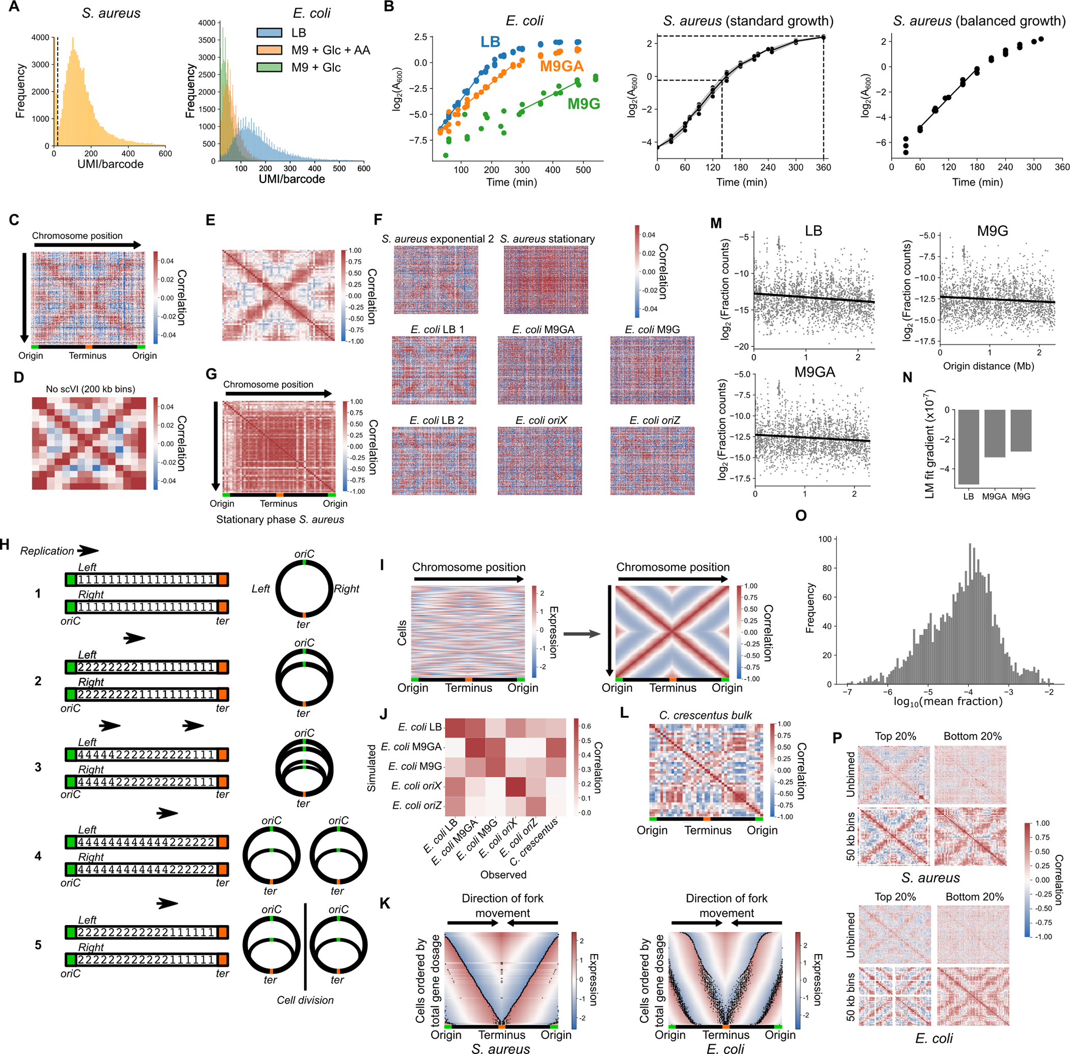
We first aimed to study gene expression at the single cell level in proliferating bacterial populations by applying the recently-described PETRI-seq¹⁸ method for scRNA-seq to S. aureus cells in exponential phase (Fig. 1A). We detected on average 135 transcripts across 73,053 individual cells (Extended Data Fig. 1A, Supplementary Table 1). As the transcriptome measurements were highly sparse, we denoised them using the single-cell variational inference (scVI) method²². Studying gene-gene correlations on a local scale, we observed the expected high correlations between the expression profiles of genes residing in the same operon (Fig. 1B). Surprisingly, when we investigated gene-gene correlations on a genomic scale, we discovered a striking “X-shaped” pattern of gene expression correlations (Fig. 1C). We can break this pattern into three major elements (Fig. 1D): 1) correlation between genes near to each other on the chromosome; 2) correlation between genes equidistant from the origin of replication; 3) correlation between origin-proximal and terminus-proximal genes. This pattern was also evident in a second independent dataset of 21,257 cells (Extended Data Fig. 1E), however we did not observe it for cells in stationary phase (Extended Data Fig. 1G), suggesting that it is a property of proliferating cells.

Fig. 1: scRNA-seq reveals a global pattern of replication-associated gene covariance.

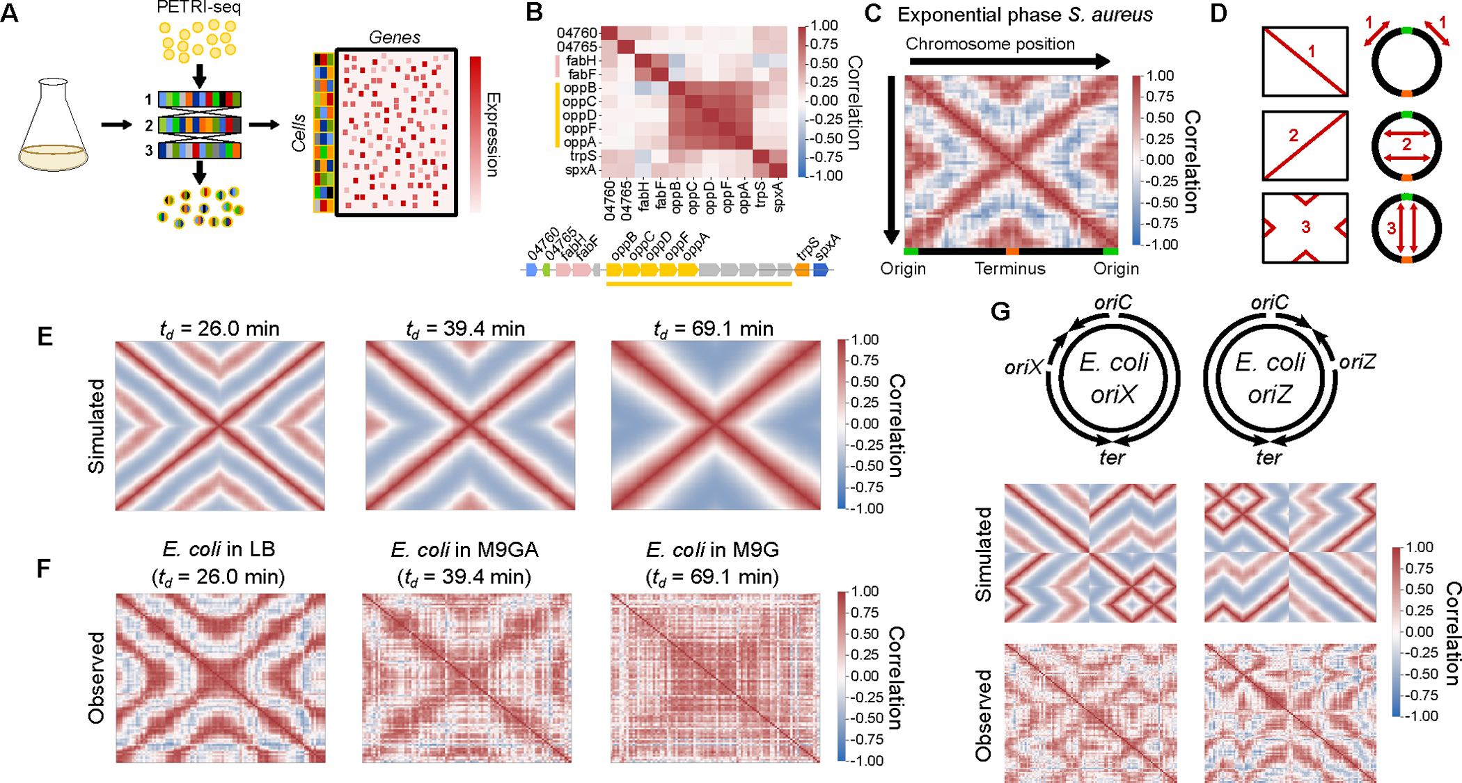
A) PETRI-seq workflow¹⁸. B) Local operon structure is captured by gene-gene correlations (Spearman’s r) in S. aureus strain USA300 LAC. Operons are indicated by shared colors of genes. Gray genes indicate those removed by low-count filtering. C) Heatmap of the global gene-gene correlations according to chromosomal position. Spearman correlations were calculated based on scVI-smoothed expression averaged in 50 kb bins by chromosome position. D) Schematic depicting the individual elements of positive gene-gene correlations in (C) according to their chromosomal locations E) Simulated correlation patterns in unsynchronized E. coli populations at three different growth rates. F) Spearman correlations between scaled data averaged into 50 kb bins, as for (C) but for E. coli grown at indicated growth rates (see Supplementary Table 1 & Methods). G) Top: schematic of predicted replication patterns in two E. coli strains with ectopic origins. Middle: Predicted correlation patterns based on the copy number simulation. Bottom: Real correlation patterns in oriX and oriZ mutant strains, as in (C).

This proliferation-dependence and correlation of genes equidistant from the origin of replication (Fig. 1D), led us to hypothesize that the “X-shaped” pattern reflects the effect of DNA replication on gene expression. In the model organism E. coli, when the cell doubling time is less than the approximately constant ~40–50 minute period for one complete round of DNA replication from the origin to the terminus (the “C-period”), simultaneous overlapping cycles of replication occur^6,23,24. This leads to growth rate dependence in replication patterns and suggests that any effects of replication on global gene correlations should also be growth rate-dependent. To test this, we developed a simulation to predict growth rate-dependent gene expression correlations arising from replication-dependent changes in gene dosage (Fig. 1E & Extended Data Fig. 1H–K). Of three growth rates simulated, the intermediate growth rate ($t_d$ = 39.4 min) led to a pattern most similar to S. aureus (Fig. 1C). However, simulating faster growth produced a nested “multi-X” pattern resulting from overlapping cycles of replication, and slower growth greatly reduced origin-terminus correlations (Fig. 1E). When we measured expression patterns in E. coli grown at these three rates, we found that each pattern closely corresponded to its respective simulation (Fig. 1F, Extended Data Fig. 1J). This and further arguments (Extended Data Fig. 1L–P & Methods) demonstrate that replication-driven gene dosage changes are a plausible mechanism driving chromosome-wide expression correlation patterns.

To further test our ability to predict global gene expression correlations from expected replication patterns, we examined strains in which normal replication is perturbed. We studied two E. coli strains with ectopic origins of replication at either the 9 o’clock (oriX) or 3 o’clock (oriZ) positions in addition to oriC^25–27. In these strains, replication was shown to initiate simultaneously at both native and inserted origins, while ending at the same terminus²⁵. Again, our simulation effectively predicted the perturbed correlation patterns in these strains (Fig. 1G). Collectively, these results support the notion that DNA replication produces a predictable effect on transcriptional heterogeneity within a population of proliferating bacteria, and that this effect is sensitive to growth rate and genetic perturbations.

Cell cycle state inference

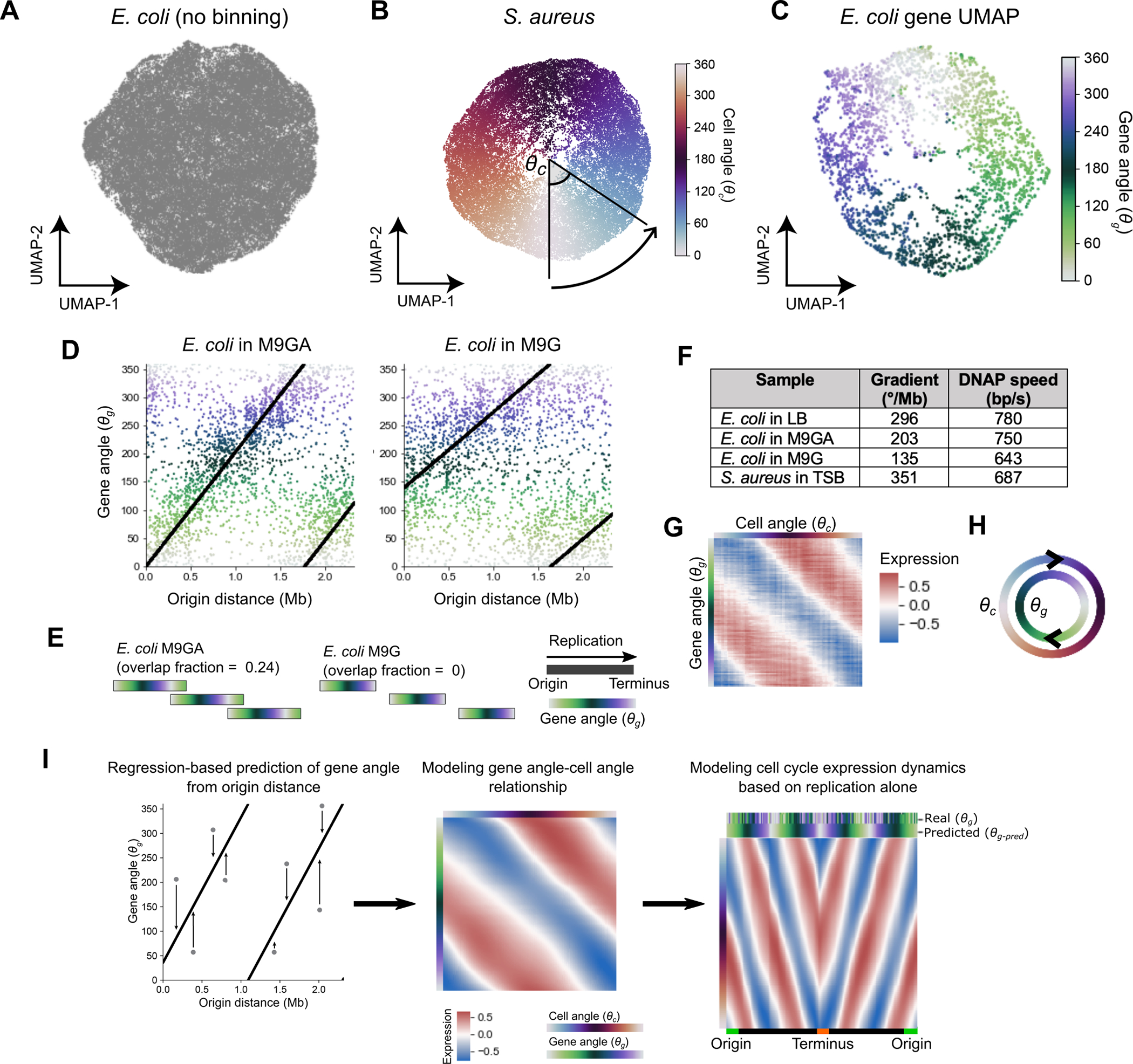
As our gene-level analysis revealed the effect of replication on gene expression, we next carried out a cell-level analysis that exploited this insight to resolve individual cells based on their replication state. To observe cell-cell relationships, we projected the transcriptomes of LB-grown E. coli cells, into a two-dimensional space, after collapsing the expression of individual genes into 100 kb regions to strengthen the chromosome position-dependent signal (as in Fig. 1C). We found a distinctive wheel-shape arrangement of the cells (Fig. 2A), indicating the capturing of a cyclical process occurring within the population. Hypothesizing that this wheel reflects the cell cycle, we computed a “cell angle” index – ${\theta }_c$ – which simply orders the cells according to their geometric angle from the center in this space. Examining gene expression as a function of ${\theta }_c$, we observed waves of gene expression progressing from the origin to the terminus (Fig. 2B), suggesting that cells’ positions on this wheel indeed reveal their replication state. Similar periodical patterns were observed in simulated data (Extended Data Fig. 1K & F) and in S. aureus cells (Fig. 2C, Extended Data Fig. 2B). These data suggest that the transcriptome alone can be used to infer a cell’s replication state, and that this holds across different bacterial species.

Fig. 2: Cell cycle analysis of bacterial gene expression.

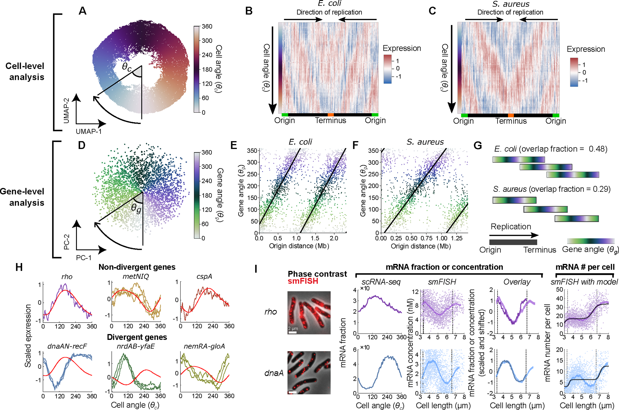
A) Two-dimensional projection by Uniform Manifold Approximation and Projection (UMAP) of LB-grown E. coli with expression averaged in 100 kb bins by chromosome position. Cell angle ${\theta }_c$ is the angle between UMAP dimensions relative to the center. B & C) Heatmaps of scaled gene expression in E. coli (B) and S. aureus (C) averaged in 100 bins by ${\theta }_c$. D) Principal component analysis at the gene level; ${\theta }_g$ is defined as the angle between principal components (PCs) 1 and 2. E & F) The relationship between ${\theta }_g$ and origin distance for E. coli grown in LB (E) and S. aureus grown in TSB (F). G) Predicted replication patterns in LB-grown E. coli and TSB-grown S. aureus. Overlapping replication rounds lead to shared ${\theta }_g$ in simultaneously-replicated chromosomal regions. H) Expression of genes in operons across 100 bins averaged by ${\theta }_c$. Expression is z-scores derived from scVI (jagged lines) or predicted as a replication effect (smooth, red lines). I) Comparison of scRNA-seq and smFISH data for two genes (see Extended Data Fig. 6A for more genes and further details). Left to right: 1) Microscopy images of E. coli cells labeled using gene-specific smFISH probes; 2) scRNA-seq expression shown as fraction of total cellular mRNA; 3) mRNA concentration, measured using smFISH, as a function of cell length. Single cell measurements are indicated alongside the moving average. Dashed lines indicate the inferred mean values at birth and division; 4) Alignment of scaled data from smFISH and scRNA-seq measurements; 5) Absolute mRNA copy number, measured using smFISH, as a function of cell length. Representative of two independent experiments.

As we observed that gene expression moved in waves during progression along the cell angle trajectory, we reasoned that we should also be able to order genes according to their expression profiles. We thus developed a similar ordering metric, which we denoted the gene angle, ${\theta }_g$ (Fig. 2D). Consistent with a role of replication in driving expression patterns, we observed a linear relationship between a gene’s ${\theta }_g$ and its genomic distance from the origin of replication in both species (Fig. 2E & F). This suggested that ${\theta }_g$ may be ordering genes according to their order of replication. The relationship however is not a simple ordering of genes from origin to terminus. For E. coli, we observed that the period of ${\theta }_g$ (i.e. the chromosomal distance associated with a 360° rotation) was much less than the full origin-terminus distance, meaning that genes at multiple positions on the origin-terminus axis had the same ${\theta }_g$ value (Fig. 2E). This intuitively relates to the fact that at high growth rates, multiple overlapping rounds of replication lead to simultaneous replication of genes at different distances from the origin. To quantify this further, we used the gradient between the ${\theta }_g$ and the distance from the origin to estimate an “overlap fraction” (Fig. 2G), meaning the fraction of one round of replication happening before the previous one has finished. When we compared E. coli at different growth rates, we observed that, in line with expectations^6,23, decreasing proliferation speed in E. coli is associated with reduced overlap in rounds of replication (Extended Data Fig. 2D & E). In S. aureus, too, we observed that genes close to the origin and terminus had similar ${\theta }_g$ values, in line with our observation of a direct correlation between genes in these regions (Fig. 1C & D). This implies that S. aureus can also exhibit multiple rounds of simultaneous replication at fast growth rates.

If the gene angle captures the order of replication of a gene then it should be possible to compute the average speed of DNA polymerase using the doubling time and the ${\theta }_g$-origin distance gradient. For E. coli in LB, this estimate was 780 bp/s (Extended Data Fig. 2F), which is very close to previously reported values of ~800 bp/s^28,29. This would correspond to a C-period of ~50 min to replicate the full 2.3 Mb distance from origin to terminus. In S. aureus, we predict a slightly slower replication speed of 687 bp/s. However, its smaller genome (1.4 Mb from origin to terminus) means that a shorter C-period (~35 min) is inferred, leading to less overlap in rounds of replication than E. coli (Fig. 2G) despite very similar doubling times. Therefore, the gene angle ${\theta }_g$ provides a quantitative and interpretable description of the relationship between gene expression and global replication patterns. Given the relationship between ${\theta }_g$ and the cell angle, ${\theta }_c$ (Extended Data Fig. 2G & H) we could therefore devise an inference model that predicts expression of a given gene (by ${\theta }_g$) at a given point in the cell cycle (by ${\theta }_c$), based purely on its distance from the origin of replication (Extended Data Fig. 2I). This model effectively captured the global chromosome position-dependent expression pattern (Extended Data Fig. 4A & B) and, crucially, gives us a baseline prediction for determining whether or not individual genes behave according to global, replication-driven trends.

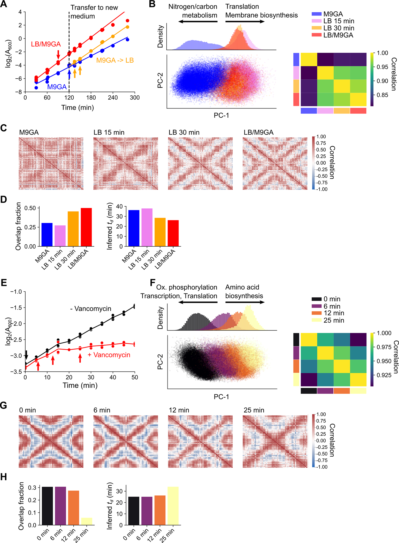
Finally, we wished to test whether we could use this framework to infer replication dynamics under changing growth rates. We considered two scenarios: a growth rate “shift-up” upon transferring E. coli into a richer growth medium³⁰ (Extended Data Fig. 3A–D) and a “shift-down” upon exposing S. aureus to high concentrations of the antibiotic vancomycin (Extended Data Fig. 3E–H). Consistent with previous observations³⁰, we found that in both cases while the transcriptional response to these stimuli happened very rapidly, the shift in the replication pattern (more- or less-overlapping in growth acceleration and deceleration, respectively), occurred only after a delay. Therefore, our analysis of replication dynamics from scRNA-seq data is not only robust to external perturbations to the global transcriptome, but also provides information on relative changes to replication patterns independent of other transcriptional changes.

Canonical and divergent gene expression

To test if the wheel-shaped distribution of cells indeed reflected cell cycle-dependent gene expression, we turned to single-molecule fluorescence in situ hybridization (smFISH)^8,31, a scRNA-Seq-independent approach that uses microscopy to detect individual transcripts in single cells. We first identified operons whose genes’ expression both did and did not fit the pattern predicted by our inference model (Fig. 2H). We then compared our measurements for genes within the selected operons to cell cycle-dependent gene expression measurements obtained using smFISH^8,31. Between scRNA-Seq and smFISH, the overall expression levels of the genes were in close quantitative agreement (Extended Data Fig. 5D). The smFISH approach resolves E. coli cell cycle states by using cell length to infer cell age, thus defining the cell cycle relative to division timing (i.e. the time since cell birth)⁸. By contrast, we defined cell angle ${\theta }_c$ = 0 to be the assumed time of replication initiation (see Methods). As expected given these differing “start” points, we observed a phase shift in expression profiles between the two methods that was consistent across genes (Extended Data Fig. 5E). Modeling of total DNA content as a function of cell length supported that this phase shift was roughly consistent with our choice of ${\theta }_c$ = 0 as the point of replication initiation (Extended Data Fig. 5F), albeit with some discrepancy (see Methods). By correcting for this phase shift between methods, we aligned the scRNA-seq profile to that of the smFISH data (Fig. 2I, Extended Data Fig. 6A). In doing so, we observed that expression dynamics inferred by the two methods were highly correlated, confirming that our scRNA-seq approach indeed captures cell cycle-dependent expression.

When we analyzed cell cycle expression patterns of genes that did and did not diverge from the expected pattern (Fig. 2H), we noted a number of key differences. Both scRNA-seq and smFISH showed that the amplitude of cell cycle expression (i.e. the relative change between cell cycle minimum and maximum expression) was higher for these divergent genes than the non-divergent ones (Extended Data Fig. 5G). Moreover, while our scRNA-seq measurements capture only relative expression of a gene as a fraction of total cellular mRNA, the smFISH experiments additionally provide us with absolute abundance (i.e. mRNA copy number). This revealed that in non-divergent genes, there was a discrete twofold stepwise increase in expression (Fig. 2I, Extended Data Fig. 6C), consistent with genes that are sensitive to gene dosage but otherwise exhibit constant transcription rates⁸. Divergent genes, however, did not conform to this simple step function (although there was variation between replicates in the low-expressed nemA, Extended Data Fig. 6A & C). These observations support an interpretation that the inference model-predicted pattern corresponds to a canonical cell cycle expression pattern driven by gene dosage: genes that fit this pattern increase in expression only upon their replication, whereas divergent genes are governed by additional factors, leading to a higher amplitude in cell cycle expression than be explained by copy number effects alone.

Expression timing and promoter distance

We next investigated those genes whose phase in cell cycle expression differed from predictions. Divergent genes can vary in phase of expression by peaking either earlier or later in the cell cycle than predicted (Fig. 3A). In E. coli, we observed a systemic bias where the majority of divergent genes showed delayed expression, meaning that the peak of expression was later than expected based upon chromosomal location (Fig. 3A). Many of these genes were encoded in large operons, such as those involved in energy biogenesis (e.g. nuo and atp operons) and cell surface synthesis (e.g. the mraZ-ftsZ operon). We found that genes with a more distal position within these operons exhibited a greater delay (Fig. 3B, Extended Data Fig. 7A). Globally, this correlation between the delay – measured as “angle difference” (see Fig. 3A, Supplementary Table 5) – and distance from the transcriptional start site (TSS) pattern was highly significant (Fig. 3C). Moreover, this delay was clearly relative to the timing of replication: in genes whose replication-predicted pattern changed in the oriZ mutant, expression also shifted in this strain such that the delay was relative to their new replication time (Fig. 3B).

Fig. 3: Intra-operon position produces a characteristic delay in expression dynamics in E. coli.

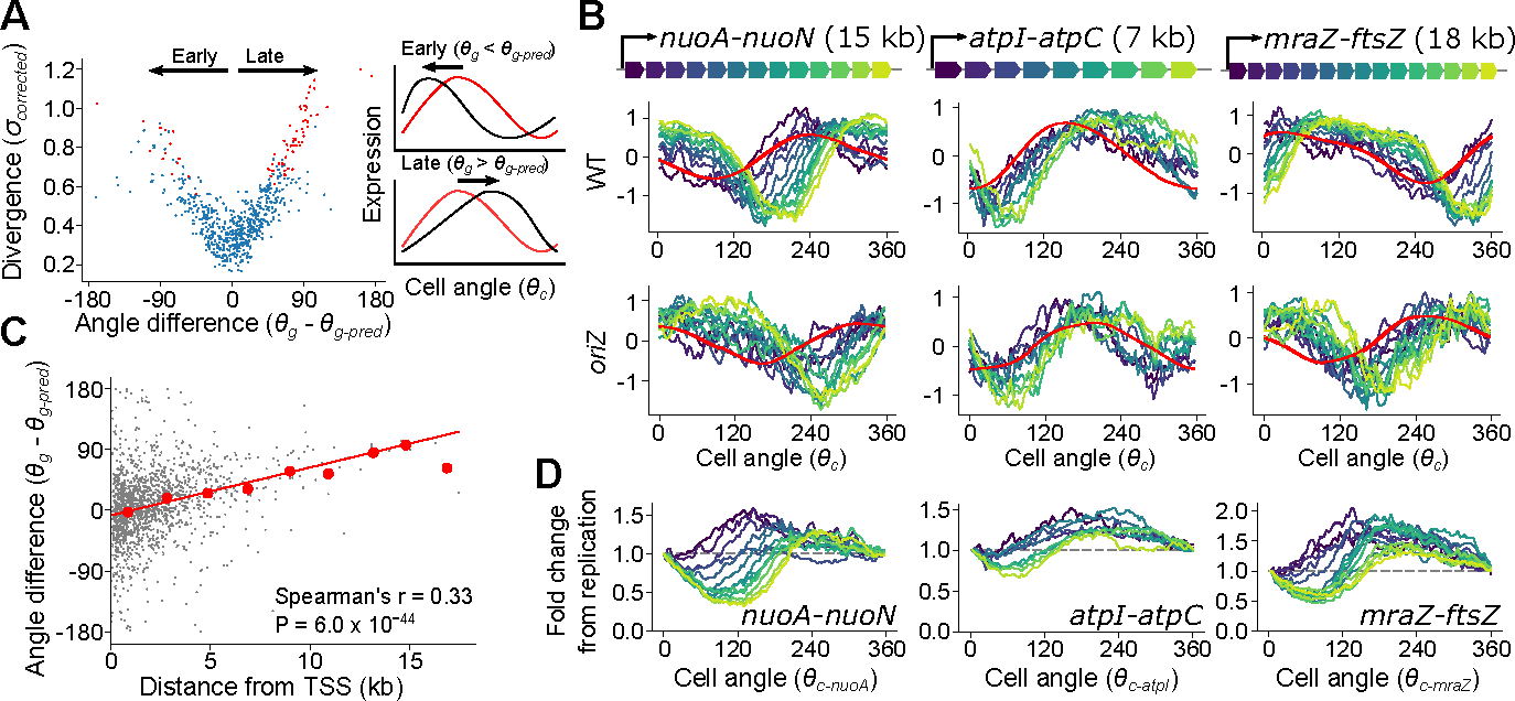
A) Left: Plot of divergence from predictions $\left.{(\sigma }_{\mathit{corrected}}\right)$ against the difference between predicted and observed angles, with divergent genes in red. Shown for all genes with high cell cycle variance (see Methods). Angle difference (${\theta }_g-{\theta }_{g-\mathit{pred}}$) represents whether a gene is expressed earlier $\left({\theta }_g<{\theta }_{g-\mathit{pred}}\right)$ or later ($\left.{\theta }_g>{\theta }_{g-\mathit{pred}}\right)$ than expected (black arrows). Right: Schematic of angle difference effects. Black and red lines represent observed and predicted cell cycle expression, respectively. B) Cell cycle expression of operons containing “delayed” genes, colored by position within the operon. Model-predicted expression is represented in red. Shown for WT and the oriZ mutant. C) Plot of distance from the transcriptional start site against angle difference. Red line indicates the linear model fit and red points indicate averages of 2 kb bins. The P-value was calculated based on a two-sided hypothesis test (see Methods). D) Fold change in expression of genes within an operon relative to expression at the operon’s predicted time of replication. Genes are colored by their position within the operon and cell angle is adjusted so that the zero point is the predicted replication time of the first gene within each operon (nuoA, atpI, mraZ). Dotted gray lines indicate the level of expression upon replication.

We hypothesized that this delayed phenotype arises due to the time for RNA polymerase (RNAP) to reach genes after replication by DNA polymerase (DNAP) has occurred. The speed of RNAP has previously been estimated as ~40 nt/s^8,32 in E. coli, much slower than the ~800 nt/s speed for DNAP^28,29 (see also Extended Data Fig. 2F). By performing linear regression to measure the angle difference/transcriptional distance relationship (Fig. 3C) and converting ${\theta }_g$ into time by assuming that 360° is equivalent to one doubling time of 26 min, we inferred that distance from the TSS is associated with a delay that is consistent with an average RNAP speed of 35nt/s (33 nt/s and 38 nt/s in two replicates, Extended Data Fig. 7C). Therefore, our data support the hypothesis that when a gene is replicated, the time for its expression to increase to the higher-expressed state (due to higher gene dosage) correlates with the time for RNAP to reach that same gene after transcription from the replicated locus restarts.

In addition to the delay, however, we also observed that when examining how expression changes after an operon is replicated, genes close to the TSS immediately increase to a new higher state, as expected from the increase in gene dosage, whereas genes far from the TSS initially drop before then recovering to the new state (Fig. 3D). This manifests as an increasing cell cycle expression amplitude (peak expression vs trough expression) of genes far from their TSS, a trend that was present as a weak but highly significant correlation across the genome (Extended Data Fig. 7D). We can interpret this effect as follows: the replication of an operon produces local disruption of ongoing transcription³³. For genes close to the TSS, expression can immediately resume at a higher rate from the duplicated locus. However, for genes far from the TSS, the new rounds of transcription may take several minutes to reach them, during which time a drop in expression is observed due to mRNA degradation. An implication of this is that internal promoters should buffer the effects of replication-associated loss of transcription. While the nuo operon contains no well-evidenced internal promoters, a substantial amount of transcription at the distal end of the mraZ-ftsZ operon is driven from internal promoters^34,35. Therefore, expression amplitude rises linearly with TSS distance in the nuo operon whereas it tails off at the location of the internal promoters within the mraZ-ftsZ operon (Extended Data Fig. 7B), supporting our inference. Thus internal promoters may prevent excessive fluctuations in key genes such as ftsZ, which determines the timing of cell division³⁶, and in principle it may even be possible to use these signatures to infer the presence of internal promoters within operons.

Finally, we asked whether similar trends could be observed in S. aureus. In contrast to E. coli, we observed neither an excess of “delayed” genes among the divergent genes (Extended Data Fig. 7F), nor an effect of distance from the TSS on expression amplitude (Extended Data Fig. 7D). We did however measure a delay as a function of distance from the TSS (Extended Data Fig. 7C), which we found to be consistent with an RNAP elongation speed of 71 nt/s (59, 64, and 92 nt/s across three replicates). The difference between the two species persisted even when operons were redefined according to unified criteria³⁷ (Extended Data Fig. 7E). The RNAP speed of S. aureus has not been measured, but in B. subtilis, which is, similarly to S. aureus, a firmicute of the order Bacillales, experimental measurement of RNAP by a reporter system suggested that it was substantially faster (75–80 nt/s) than its counterpart in E. coli measured by the same method (~48 nt/s)^38,39. Therefore, we tested whether we could use our method to detect this faster RNAP speed in B. subtilis (Extended Fig. 8). Despite multiple additional sources of heterogeneity in this species – including multicellular chain growth, prophage activation and sporulation programs¹⁹ – we nevertheless resolved a highly overlapping replication pattern (Extended Data Fig. 8D & E) from which we inferred a DNAP speed of 632 bp/s (631 and 634 bp/s across two replicates), which is close to that of S. aureus and, as previously reported⁴⁰, ~80% of the E. coli speed. However, as predicted, we estimated a faster RNAP speed for B. subtilis of 96 nt/s (Extended Data Fig. 8G) (95 and 98 nt/s in two replicates). Similar trends could be observed across species for individual long operons (Extended Data Fig. 8I). Therefore, the intra-operon effect we observe in E. coli is not conserved across species, and likely follows from variation in RNAP elongation speed.

Repression-driven expression pulses

Our analysis above revealed recurrent, replication-coupled patterns of cell cycle expression. To enable comparison of replication-coupled expression dynamics across different chromosomal loci, we aligned their mean-standardized expression profiles such that zero on the x-axis represents the point of a gene’s replication and ${\theta }_{c-rep}$ the cell cycle progression from this point (Fig. 4A). We refer to this as the “Transcription-Replication Interaction Profile” (TRIP) and propose that it enables an explicit focus on the transcriptional response of each gene to the perturbation caused by its replication, independent of when in the cell cycle that gene is replicated. Among genes whose cell cycle expression was reproducible across replicates (Supplementary Table 6), the profile for most genes was similar, rising rapidly due to a doubling of gene dosage before declining as a relative fraction of the transcriptome as other genes are replicated and hence increase their own fractional abundance. Many genes, however, exhibited patterns that could not be explained by gene dosage effects alone.

Fig. 4: Transcription-replication interaction profiles (TRIPs).

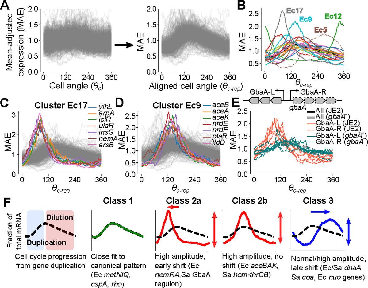
A) Procedure to generate TRIPs. Expression is mean-adjusted by division of each gene by its mean (left), then aligned by rotating cell angle so the predicted replication time expression is at zero (see Methods). B) Average aligned expression profiles for 20 k-means clusters in E. coli. The dotted black line represents average expression across all reproducible genes. C & D) Plots of individual genes from the indicated clusters. E) TRIPs for GbaA regulon genes in JE2 and a gbaA⁻ (SAUSA300_RS13960) transposon mutant. Operon structure is shown above. Thick black and gray lines represent average expression across all reproducible genes. F) TRIP Classes. Left: Canonical TRIP driven by gene dosage. Other panels: Archetypal classes of TRIPs that adhere to (Class 1) or diverge (Classes 2–3) from this pattern. Genes in E. coli and S. aureus are represented as Ec and Sa, respectively.

To identify the range of behaviors, we partitioned E. coli genes into 20 clusters based on their TRIPs (Fig. 4B). Of these, several exhibited particularly divergent expression, differing from the expected pattern in both the timing of their dynamics (e.g. when their peak or trough expression occurs) and the amplitude (i.e. the relative difference between maximum and minimum cell cycle expression). Cluster 12 in E. coli (Ec12) comprised the nrdAB-yfaE operon and cluster Ec5 contained the dnaAN-recF operon and other delayed expression genes, including some nuo genes. Cluster Ec17 showed an early-peaking pulse in expression with greater amplitude than most genes (Fig. 4C). Many genes in these clusters were in operons that encode repressors, at least some of which have autorepressive activity (including nemA, which is co-transcribed with the autorepressor nemR) (Supplementary Table 4). Cluster Ec9, whose members peak at the expected time but show increased amplitude (Fig. 4D), also included several repressed genes (Supplementary Table 4), such as the glyoxylate shunt operon, aceBAK, which is IclR-repressed. Other clusters composed of low-expressed genes showed similar trends (Extended Data Fig. 9A), and low-expressed clusters that showed high amplitude were enriched for repressor targets (FDR = 0.1, Extended Data Fig. 9B). This suggested a broad association between repression state and replication-associated pulses in gene TRIPs.

When we extended this analysis to S. aureus, we noted extreme divergence in TRIP clusters within the core genes of genome-integrated mobile genetic elements (MGEs) (Extended Data Fig. 9E & F). Beyond MGE genes, however, a range of behaviors were evident, similar to those observed in E. coli (Extended Data Fig. 9C). For example, we observed high amplitude and delayed dynamics in cluster S. aureus (Sa) 9, comprised of dnaAN, as well as several high-amplitude clusters (Extended Data Fig. 9D). Sa18 was almost exclusively composed of genes in the GbaA regulon (Extended Data Fig. 9G). In contrast, cluster Sa12 showed delayed dynamics (Extended Data Fig. 9D). Notably, this included several genes involved in stress and virulence.

We reasoned that transcriptional repression could be driving the high amplitude pulses observed for TRIPs of genes in certain clusters (Ec9, Ec17, Sa11, Sa18), because of the enrichment of repressors and the low expression levels among high-amplitude clusters (Extended Data Fig. 9A & B), and based on previous observations^8,41,42. Therefore, we focused on genes of the S. aureus GbaA regulon (Extended Data Fig. 9G), which showed a particularly strong early pulse in expression. This regulon consists of two oppositely-oriented operons (referred to here as “GbaA-L” and “GbaA-R”, Fig. 4E) that are repressed by GbaA. GbaA is an electrophile-sensitive transcriptional repressor encoded by gbaA within the GbaA-R operon^43,44. To test whether GbaA repression was responsible for the divergent dynamics of its regulon, we compared wild-type TRIPs to those of a gbaA transposon mutant, where GbaA-mediated repression should be relieved. Since transposon insertion happens within the GbaA-R operon, transcription of this locus was disrupted. However, in the GbaA-L operon we observed a >100-fold increase in expression (Extended Data Fig. 9H) due to loss of repression. As predicted, this loss of repression was accompanied by a clear reversion of GbaA-L TRIPs to the expected pattern in the transposon mutant, as well as reduced expression amplitude (Fig. 4E). To further verify that relief of GbaA repression at the promoter was directly responsible for this change, we measured transcription of a reporter gene from the GbaA-L promoter at an alternative chromosomal locus. While repression by GbaA was less efficient at this locus than for native GbaA-L (Extended Data Fig. 9I), we nonetheless observed a spike in reporter expression on a wild-type JE2 background that was GbaA-dependent (Extended Data Fig. 9J). These observations suggest that repression drives the high-amplitude pulses in expression seen for low-expressed genes.

By comparing TRIPs across the genome, we identify several archetypal classes (Fig. 4F). Class 1 TRIPs reflect the canonical dosage-driven response. For genes outside this category, we observe divergence of TRIPs along two main axes: heterochrony, or differential expression phase (i.e. timing of expression changes), and heterometry, or differential amplitude (or “peak/trough ratio”). Many repressed operons exhibit heterometry (Class 2a & 2b), while a subset of these peak earlier than expected (heterochrony) (Class 2b). Genes can also exhibit heterochrony as a “delayed” expression profile (Class 3). Each class of TRIP may therefore reveal distinct features of local gene regulatory contexts.

Biophysical modeling of TRIPs

The presence of shared classes among TRIPs may suggest recurrent mechanistic drivers. To explore these hypothetical mechanisms in a quantitative manner, we interpreted the expression patterns using several biophysical models for cell-cycle dependent transcription. We first leveraged the procedure developed above of aligning scRNA-seq and smFISH data (Fig. 2I) to convert our E. coli scRNA-seq measurements (fraction mRNA as a function of ${\theta }_c$) to the estimated absolute mRNA copy number as a function of time since the last cell division (Extended Data Fig. 10A). This produced traces analogous to those measured by smFISH (Fig. 2I and Extended Data Fig. 6C). We next fitted those traces to a biophysical model¹¹ where mRNA production rate is proportional to gene dosage. In this model, gene replication at time $t_r$ results in the doubling of mRNA level over a time inversely proportional to the mRNA degradation rate k_d (Fig. 5). We found that 39% of reproducible genes were well fitted by this model (Extended Data Fig. 10B, C & I), with good consistency between replicates (Extended Data Fig. 10B). Moreover, the fitted values of k_d were significantly correlated with published values (Extended Data Fig. 10D), and the inferred replication times, $t_r$, mirrored the expectations based on each gene’s chromosomal location (Extended Data Fig. 10E). Thus, a large proportion of genes evaluated show cell cycle-dependent expression that is consistent with a simple biophysical model of dosage-dependent transcription.

Figure 5: TRIP classes can be explained by simple biophysical models of expression.

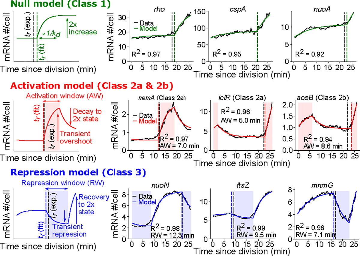
Fits of gene expression patterns to biophysical models of cell-cycle dependent transcription. Gene expression data from E. coli grown in LB was converted to absolute mRNA copy number as a function of time (see Methods). Black traces show observed expression, colored lines represent model fits. Vertical dashed lines indicate expected replication times based on predicted minimum gene expression (based on chromosome position) ($t_r$ (exp.), black lines) or based on biophysical model fits ($t_r$ (fit), colored lines) (see Methods). For each model, the left column is a schematic description of the fit and how it relates to model parameters (the “null” model parameters also apply to the expanded “activation” and “repression” models). The accompanying panels show these fits for individual genes (for two of these genes, nemA and nuoN, alternative plots of poorly fitting models are shown for comparison in Extended Data Fig. 10K).

To capture the dynamics of the TRIPs of genes with more complex expression patterns, we expanded our modeling approach. TRIP classes 2a & 2b exhibit “pulses” of expression upon replication (Fig. 4F). We thus developed an “activation model” in which mRNA production rate transiently increases upon replication before mRNA abundance decays back to a level driven by gene dosage (Fig. 5). Genes in high amplitude expression clusters Ec17 (Fig. 4C e.g. nemA, iclR) and Ec9 (Fig. 4D e.g. aceB) had a good fit (R² > 0.9) and well-predicted gene replication times, $t_r$ (Extended Data Fig. 10H), but were poorly fitted by the null (dosage-driven) model (Extended Data Fig. 10G). Genes fitting to the activation model were also enriched for repressors (P < 10⁻⁴, hypergeometric test as in Extended Data Fig. 9B), whereas genes fitting to the null model were not (P = 1.00). Moreover, expression of lacZ was best-described by the activation model (Extended Data Fig. 10L). Previously, Wang and colleagues⁸ observed a replication-associated pulse in lacZ expression associated with the activity of its repressor, LacI, further supporting our inference that many genes fitting to the activation model are in a repressed state. Finally, the activation model enabled us to interrogate what determines whether a gene displays early-peaking behavior (Class 2a) or not (Class 2b). The IclR regulon encompasses both its own gene, iclR, and the neighboring aceBAK operon. While iclR peaks early (Class 2a, Fig. 4C), aceBAK genes peak at the expected time (Class 2b, Fig. 4D). In this case, model fits suggested that this difference is driven by a longer activation window for aceBAK, implying that it takes longer for IclR-dependent repression to be restored at aceBAK than at iclR (Extended Data Fig. 10N). Therefore, analysis of model fits can suggest useful hypotheses regarding specific regulatory circuits.

Neither of these models, however, can accurately describe genes with delayed expression timing (“Class 3” TRIPs). Specifically, each fails to predict the replication timing both in the delayed cluster Ec5 (Fig. 4B, Extended Data Fig. 10H) and for genes far from their promoter (Extended Data Fig. 10J). Since many of these genes show a drop in transcript abundance upon replication (Fig. 3D), we introduced a “repression model” that features a transient window of reduced mRNA production rate upon gene replication. This model effectively captured genes distant from their TSS, including for those genes at the far end of nuo and mraZ-ftsZ operons (Fig. 5, Extended Data Fig. 10J), while the promoter-proximal nuoA was sufficiently described by the null model (Fig. 5). Other genes with a “delayed” (Class 3) TRIP that were well-described by the repression model included genes immediately adjacent to the oriC locus (mioC and mnmG, Fig. 5, Extended Data Fig. 10M), as well as dnaA (Extended Data Fig. 10M), all of which have previously been suggested to experience transient repression around the time of their replication^45,46. Of the genes not captured by the null model, the repression model explained fewer genes than the activation model, and most of the former genes’ repressed dynamics can be linked to their position within operons (Extended Data Fig. 10I). Thus, replication-dependent repression for other reasons appears to be a relatively unusual phenomenon. Overall, the simple biophysical modeling provides gene-level estimation of testable gene regulatory parameters, including mRNA decay, transcription activation and repression.

Discussion

Here we reveal the cell cycle transcriptional dynamics of rapidly dividing bacteria. Our work differs substantially not only from scRNA-seq analysis of cell cycle phase-specific genes in eukaryotic cells⁴⁷, but also from previous studies of cell cycle transcriptomes in bulk, synchronized bacterial populations. It was previously suggested that, at least for ɑ-proteobacteria^12,15, transcription of cell cycle genes was temporally regulated according to function. Our observations, however, suggest that the more general situation in prokaryotes, at least under rapid growth conditions, is one where cytoplasmic content is relatively invariant throughout the cell cycle⁴⁸, and rather that the major perturbation to gene expression is the local effect of chromosomal replication itself. For example, cell cycle fluctuation in mRNA of ftsZ, the major cell division regulator, was described previously^49,50. A direct link between ftsZ replication and transcriptional inhibition was postulated⁵⁰, but the authors could not provide a satisfactory mechanistic explanation. Here, we provide a simple explanation of these augmented fluctuations in ftsZ abundance as the natural consequence of replication of a gene transcribed from a distant promoter (Fig. 3D), and not due to a cell division-coupled signaling event. While global factors may still play a role, such as competition for RNA polymerase between genes⁵¹, our work points to a central role of gene replication in driving cell cycle transcriptional dynamics.

We introduce the notion of the TRIP as a gene-level summary of the response of each gene to the perturbation of its own replication. This profile is analogous to the electrocardiogram (ECG), a time-resolved electrical pattern whose sophisticated, quantitative interpretation yields a wealth of information about cardiac function. Similarly, by continuing to refine the capture and analysis of TRIPs we expect to gain an ever more detailed diagnostic picture of gene regulation. Presently, we can distinguish a number of broad classes of TRIPs (Fig. 4G). For many genes, expression changes upon replication are sensitive primarily to copy number increases, and their dynamics can be described simply by their mRNA production and decay rates, as well as their replication timing. Other classes exhibit heterometry (here, primarily high amplitude) and heterochrony (early or delayed expression) that reveal important features of their regulatory environment, from repression state to promoter usage. These models, however, can be extended to other regulatory motifs. For example, many operons with genes displaying particularly strong “pulses” of expression upon replication are under autorepression (Supplementary Table 4), a network motif that facilitates rapid peaking of expression⁵². Biophysical models that can account for these specific motifs will allow us to both test and generate increasingly specific hypotheses about the regulatory context of a gene. While a gene’s fit to a specific biophysical model does not automatically entail a specific regulatory mechanism, nevertheless it places constraints on the plausible molecular processes leading to that TRIP. Crucially, the ability to reveal regulatory motifs without genetic perturbations, as well as to infer relevant global parameters such as DNAP and RNAP speeds, will allow expansion of our approach across non-model organisms or strains where the regulatory network is poorly characterized. We expect that the rapid improvement in scale and capture efficiency of bacterial scRNA-seq methodologies^4,53–55 will allow us to perform ever deeper and more quantitative analyses.

Single cell analysis of eukaryotic cells has led to the development of a suite of analysis tools based principally on clustering and interpreting cell populations from specific marker genes⁵⁶. While these approaches may be applicable to prokaryotes in certain circumstances, a hallmark of bacterial systems biology has been the use of quantitative, model-driven analysis of gene regulation and physiology^2,57. This arises from both the simplicity of bacteria and the reproducibility - with careful experimental design - of bacterial measurements. Physically-inspired modeling has been applied to eukaryotic scRNA-seq, particularly in the context of RNA velocity⁵⁸, but in practice these approaches are typically used to infer cellular behaviors such as developmental processes⁵⁹. Our work demonstrates that bacterial scRNA-seq can produce quantitative estimates of molecular-level dynamics on a genome-wide scale and in a wide range of organisms. Our cell cycle analysis and TRIP frameworks, however, are likely only the first examples of such quantitative analyses now enabled by single-cell technologies.

Methods

Bacterial strains and media

Strains used are listed in Supplementary Table 1. All E. coli strains (a gift from Dr. Christian Rudolph) and B. subtilis (ATCC) were routinely grown in modified Luria Broth (LB) (1% tryptone (Sigma-Aldrich), 0.5% yeast extract (Sigma-Aldrich), 0.05% NaCl, pH adjusted to 7.4)²⁶. For growth in minimal media, an M9 base (1X M9 minimal salts (Gibco), 2 mM MgSO₄, 0.2 mM CaCl₂) was supplemented with 0.4% glucose (M9 + glucose: M9G) or with both 0.4% glucose and 0.2% acid casein peptone (Acros Organics) (M9 + glucose + amino acids: M9GA). All S. aureus strains were routinely grown in Bacto tryptic soy broth (TSB) (BD Biosciences). The gbaA transposon mutant was provided by the Biodefence and Emerging Infections (BEI) Resources Repository (cat. # NR-46898).

Growth curves and harvesting for PETRI-seq

All growth experiments were performed at 37° with shaking at 225 rpm.

Constant growth conditions

Strains were grown overnight in LB (E. coli & B. subtilis) or TSB (S. aureus). For initial experiments with S. aureus (Datasets D3 & D4), strains were diluted to an A₆₀₀ value of 0.05 in prewarmed TSB, after which A₆₀₀ was measured at the times specified. A₆₀₀ was measured on a BioMate 3S spectrophotometer (Thermo Scientific). For experiments with S. aureus in balanced growth (Datasets D5-D8), overnight cultures were diluted in TSB first to 0.005, then after 3 hr diluted again to 0.005 before measuring A₆₀₀ at the time intervals specified. Growth of B. subtilis was the same except with LB used as the growth medium. For E. coli growth curves, strains were diluted to an A₆₀₀ value of 0.05 and incubated for 2 hr in the desired medium then diluted again in the same prewarmed medium to an A₆₀₀ value of 0.005, after which A₆₀₀ was measured at the time intervals specified. Where E. coli cells were diluted into a different medium, cells were washed once with PBS prior to dilution. To measure growth rate, a linear model log₂(A₆₀₀) ~ mT + c was calculated for the linear portion of this relationship (where T is the time in minutes) using the LINEST function in Microsoft Excel and the doubling time in minutes $t_d$ was calculated as 1/m. All doubling times are provided in Supplementary Table 1.

For harvesting for PETRI-seq, cells were grown as described except that after specific time intervals (for S. aureus, 2 hr 20 min in initial experiments, 1 hr 30 min in balanced growth experiments; for E. coli, 2 hr, 3 hr, and 7 hr in LB, M9GA, and M9G, respectively, when growth rates appeared constant (Extended Data Fig. 1B); for B. subtilis, 1 hr 30 min) cells were harvested by centrifugation and resuspension in 4% formaldehyde in PBS. For S. aureus initial experiments, centrifugation was at 10,000 × g, 1 min at room temperature and for E. coli, B. subtilis, and balanced growth S. aureus experiments, centrifugation was at 3,220 × g, 5 min, 4°C. For B. subtilis, because sensitivity in the transcriptome to cold shock was previously noted upon gradual cooling during centrifugation at 4°C¹⁹, cells were initially cooled to <10°C by rapid agitation in a dry ice ethanol bath followed by retention on ice to prevent further transcriptional changes after harvesting.

For growth under perturbed conditions, see SI Methods Section “Growth perturbation conditions”.

PETRI-seq

PETRI-seq was carried out as described previously¹⁸ with modifications as described in the SI Methods Section “PETRI-seq modifications”.

Analysis of PETRI-seq data

Pre-processing of scRNA-seq data

Initial demultiplexing of barcodes, alignment, and feature quantification was performed using the analysis pipeline described in ¹⁸ except that feature quantification was performed at the gene level rather than operon level. Reference sequences and annotations were obtained from Genbank (https://www.ncbi.nlm.nih.gov/genbank/). E. coli reads were aligned to the K-12 MG1655 reference assembly (GCA_000005845.2), S. aureus to the USA300_FPR3757 reference assembly (GCF_000013465.1), and B. subtilis to the 168 reference assembly (GCF_000009045.1). After initial processing, counts by cell barcode were pooled across different libraries (no batch effects were noted between libraries) and initial filtering was performed using Scanpy v1.7.1⁶⁰. Barcodes with UMI below a threshold (10 for Dataset D9 rep 2, 15 for Dataset D1, D2, D4, and D10 (all samples but M9GA); 20 for Dataset D3, D5–7, D9 rep 1, and D10 M9GA, 40 for Dataset D8) were removed, as well as any genes with fewer than 50 UMI across all included barcodes (100 for Dataset D3 & D9). Note that within the main text, we refer to UMI as simply “transcripts” for the sake of clarity, although we acknowledge that with random priming more than one unique read could originate from a single mRNA molecule.

Data denoising and generation of gene-gene correlations

To generate the denoised representation of the data, scVI v0.9.0²² was applied with the following hyperparameters, chosen through grid search to distinguish between closely related S. aureus strains in a pilot dataset: two hidden layers, 64 nodes per layer, five latent variables, a dropout rate of 0.1, and with a zero-inflated negative binomial gene likelihood (other hyperparameters maintained as defaults). The model was trained with default parameters. Denoised expression values based on the scVI model were obtained using the scVI function “get_normalized_expression”. Initial gene-gene correlations without binning (Extended Data Fig. 1C & F) were calculated from scVI-normalized counts using the “get_feature_correlation_matrix” function. For correlations with position-dependent binning, scVI-normalized expression matrices were first log₂-transformed and then converted to z-scores by mean centering followed by division by the standard deviation. For Extended Data Fig. 1D, this was carried out using raw counts normalized by total UMI per cell, and transformation by log₂(x + 1) (to allow for zero values). After removing extrachromosomal genes, expression z-scores were averaged within bins (50 kb unless otherwise stated) and Spearman correlations between bins were calculated. For B. subtilis analysis, UMAP of initial scVI smoothed data revealed two clusters in initial analysis, with one cluster arising due to PBSX mobilization (Extended Data Fig. 8C). To generate the final scVI models, we removed this cluster and repeated scVI on the remaining cells. Note that for PBSX annotation and for annotation in S. aureus MGEs (Extended Data Fig. 9F), the online tool Phaster⁶¹ (phaster.ca) was used. For further discussion of evidence supporting our analysis of global gene correlations, see SI Methods Section “Quality assessment of global correlations in gene expression”.

Cell cycle analysis

Our quantitative framework describing gene expression as a function of replication cycle state (Fig. 2) is parameterized as the relationship between gene expression and two further parameters, cell angle ${\theta }_c$ (describing the position of cells within the cell cycle) and gene angle ${\theta }_g$ (describing the ordering of expression of genes within the cell cycle).

Derivation of cell angle, ${\theta }_c$.

The position of cells within the cell cycle was determined as follows. First, scVI-derived z-scores (Section ”Data denoising and generation of gene-gene correlations”) were averaged into bins according to chromosomal location (50–400 kb bins, depending on the dataset). Binned data were then projected into two dimensions by UMAP analysis using the umap-learn v0.5.1 library in Python (https://umap-learn.readthedocs.io/en/latest/) with the “correlation” distance metric, generating the “wheel” plots shown (Fig. 2A & Extended Data Fig. 2B). To assign cells to a particular replication cycle phase based on their position, the embeddings were first mean-centered and then the angle of each cell ${\theta }_c$ relative to the origin between x and y coordinates in a two-dimensional UMAP embedding was calculated as tan⁻¹(x / y), similar to the ZAVIT method our lab has described previously^62,63. To get the expression by cell angle matrix used in Fig. 2B & C, scVI-denoised gene expression z-scores were then averaged within 100 equally spaced bins of ${\theta }_c$ to produce a cell angle-binned expression matrix. For UMAP without averaging, see Extended Data Fig. 2A.

Derivation of gene angle, ${\theta }_g$.

After averaging gene expression within 100 equally spaced bins of ${\theta }_c$ (as in Fig. 2B & C), principal component analysis (PCA) was performed on the transpose of this matrix to generate a low-dimensional projection of genes based on their cell cycle expression (Fig. 2D). Analogous to the derivation of ${\theta }_c$, gene angle ${\theta }_g$ was calculated as the angle between PCs 1 and 2 relative to the origin. As discussed, this parameter roughly relates to genes’ order of expression within the cell cycle and indeed recapitulates the order in which genes are replicated (Fig. 2E & F). We chose to use PCA instead of UMAP to derive ${\theta }_g$ because while UMAP produces a “wheel” similar to the cell-level analysis (Extended Data Fig. 2C), we reasoned that as a linear dimensionality reduction PCA would be more likely to give a consistent gene angle/origin distance relationship. However PCA-derived ${\theta }_g$ values still broadly capture the ordering when UMAP is performed (Extended Data Fig. 2C).

Predicting expression dynamics based on DNA replication alone

We developed two regression models to infer predicted a gene’s predicted gene angle ${\theta }_{g-pred}$ from its distance from the origin of replication (SI Methods Section “Modeling the gene angle-origin distance relationship”) and then to predict cell cycle expression from this ${\theta }_{g-pred}$ value (SI Methods Section “Modeling the cell angle-gene angle relationship”). These models were combined to yield the pipeline in Extended Data Fig. 2I. Firstly, the gene angle-origin distance model (SI Methods Section “Modeling the gene angle-origin distance relationship”) was used to predict the expected value ${\theta }_{g-pred}$ from origin distance D. Next, cell cycle expression was predicted using the cell angle-gene angle regression model (SI Methods Section “Modeling the cell angle-gene angle relationship”) using ${\theta }_{g-pred}$ values. For cell angle ${\theta }_c$, values used were the average ${\theta }_c$ values of cells binned into 100 equally spaced bins by ${\theta }_c$. This gives a replication-predicted gene expression matrix of 100 bins × number of genes. The success of this model fit was evaluated based on the correlation with the ${\theta }_c$-binned expression z-scores derived from scVI (Extended Data Fig. 4A & F), as well as the loss of global chromosome position-dependent gene-gene correlations upon correction of scVI expression with replication-predicted expression (Extended Data Fig. 4B & G). Additionally, we used this modeling approach to set the zero angle for gene expression plots.

Setting the position of ${\theta }_c=0.$

Initially, the cell angle ${\theta }_c$ orders cells by their cell cycle position within a circle but the start point, when ${\theta }_c=0$, is arbitrary. This is not only challenging to interpret but impedes comparing across replicates. Therefore, we standardized ${\theta }_c$ so that ${\theta }_c=0$ was the predicted point of replication initiation. Using the inference approach described above, we predicted the gene expression profile by ${\theta }_c$ for an imaginary gene at $D=0$ (i.e. at the origin of replication). We then determined the value of ${\theta }_c$ giving the minimum predicted expression, reasoning that if increased expression in this model is responsive to a doubling of copy number, the doubling event should occur approximately at the expression minimum. Therefore, we determined this angle, ${\theta }_0$ to be the most likely value of ${\theta }_c$ at which replication initiation occurs, rotating the angles by the operation (${\theta }_c-{\theta }_0$) mod 360 to set this point as 0°. This interpretation is roughly in accordance with the estimated timing of replication initiation as determined directly from smFISH data (Extended Data Fig. 5F and SI Methods Section “Inferring cell-cycle phase from the DAPI signal”). Crucially, however, it also provides a point of standardization that allows in-phase comparison of cell cycle expression profiles across independent replicates.

Identifying replication-divergent genes

We identified replication-divergent genes based on two criteria: absolute variability by cell angle ${\theta }_c$ and divergence from the replication model. For details, see SI Methods Sections “Identifying genes with high cell cycle variance” and “Identifying genes with high divergence from predicted expression”.

Plotting expected and observed cell cycle expression patterns.

To visualize the degree of divergence from predicted expression, (e.g. Fig. 2H, Fig. 3B), we take scVI-derived z-scores averaged in 100 bins by ${\theta }_c$ along with model predictions (Section “Predicting expression dynamics based on DNA replication alone”). We then adjust ${\theta }_c$ as described above (Section “Setting the position of ${\theta }_c$ = 0”). Importantly, we are able to validate our analysis from the raw (non-scVI-derived) data by averaging normalized counts ${\theta }_c$ (Extended Data Fig. 4J). This demonstrates that cell cycle expression patterns are not an artifact of scVI denoising.

Analyzing the effect of operon gene position on expression dynamics

We identified the excess of genes with a “delayed” expression profile by calculating the angle difference as ${tan}^{-1}\left(sin\left({\theta }_g-{\theta }_{g-\mathit{pred}}\right)/cos\left({\theta }_g-{\theta }_{g-\mathit{pred}}\right)\right)$ where ${\theta }_g$ and ${\theta }_{g-\mathit{pred}}$ are the observed and predicted gene angles in radians, respectively. For operon annotations, E. coli and B. subtilis transcription units from Biocyc ^64,65 (https://biocyc.org/) were used. To investigate the relationship between gene distance from transcriptional start sites and angle difference in E. coli, all genes in polycistrons (transcription units with more than one gene) were included. The distance was measured from the annotated transcription unit start site to the midpoint of each gene. Where genes were in multiple transcription units, the longest distance from a start site was taken. Angle difference was converted into time by dividing the angle by 360° then multiplying by the doubling time in seconds. For S. aureus, operon annotation was obtained from AureoWiki⁶⁶ (aureowiki.med.uni-greifswald.de). Since this provided only the genes within an operon and not its start, the first base of the first gene was taken as the transcriptional start site.

Analysis of operon expression trends relative to timing of operon replication.

For each operon shown (Fig. 3D), the predicted replication timing in degrees of ${\theta }_c$ was calculated as the predicted minimum in expression for the first gene in that operon (similar to calculation of TRIPs, Section “Defining gene Transcription-Replication Interaction Profiles (TRIPs)”). The cell angle, ${\theta }_c$, was then redefined such that ${\theta }_c=0$ is the point of operon replication (denoted ${\theta }_{c-\mathit{nuoA}},$ ${\theta }_{c-\mathit{atpl}}$, and ${\theta }_{c-\mathit{mraz}}$ for each operon). With an expected DNA polymerase speed of ~800 bp/s^28,29, replication of the whole operon is expected to take <20 s so it is assumed that genes within the operon are replicated simultaneously. Next, $\mathrm{s}\mathrm{c}\mathrm{V}\mathrm{I}$-derived normalized expression of the nuo, atp, and mraZ-ftsZ operons, averaged in 100 bins by ${\theta }_c$, was converted to fold change relative to the replication point by dividing cell cycle expression by when ${\theta }_{c-\mathit{nuoA}},$ ${\theta }_{c-\mathit{atpl}}$, or ${\theta }_{c-\mathit{mraz}}$, respectively, were equal to zero degrees. As shown in Fig. 3D, this reveals that genes far from, but not close to, the TSS display transient decreases in expression.

For analysis of correlations between a gene’s position within its operon and its expression timing or amplitude, Spearman correlations were calculated using the “spearmanr” function in the Python package scipy v1.9.3⁶⁷. This function was also used to calculate P-values based on a two-sided test with the null hypothesis of no correlation.. See documentation in https://docs.scipy.org/doc/scipy/reference/generated/scipy.stats.spearmanr.html for details.

Defining gene Transcription-Replication Interaction Profiles (TRIPs)

Our work uncovered evidence that cell cycle-dependent fluctuations in each gene’s expression can arise from the diverse responses of that gene to perturbation by replication. Therefore, we define the TRIP as a gene’s expression profile relative to its predicted timing of replication. We did this for all genes that showed good reproducibility between replicates (Spearman correlation > 0.7 between expression averaged in 100 bins by ${\theta }_c$. To produce each gene’s TRIP, we first take scVI-normalized expression and average in 100 positions by ${\theta }_c$. To preserve information on the dynamics of each gene (since amplitude in cell cycle fluctuations is an important parameter in interpreting TRIPs), we do not log-transform or scale expression but instead divide by the mean expression across the cell cycle (to allow comparison of genes with different baseline expression levels). For each gene, we then determine the predicted timing of replication as the minimum in the predicted expression (Section “Predicting expression dynamics based on DNA replication alone”). We then rotate ${\theta }_c$ for that gene so that ${\theta }_c$ = 0 corresponds to this predicted replication timing. We denote this as ${\theta }_c-rep$, calculated by the transformation (${\theta }_c-{\theta }_{c-min}$) mod 360 where ${\theta }_{c-min}$ is the predicted expression minimum. Therefore, the TRIP preserves replication dynamics while allowing standardization across different replication timings and baseline expression values.

Clustering of TRIPs.

Reproducible genes were clustered based on the TRIPs derived as above using k-means clustering. TRIPs for genes within each cluster were then averaged to give the cluster profiles in Fig. 4 and Extended Data Fig. 9. To analyze for enrichment of repressed genes in E. coli, repressor annotations were obtained from Biocyc^64,65 (https://biocyc.org/). We then assessed whether genes within each cluster were enriched for genes that had an annotated repressor, using the hypergeometric test to assess significance. Since we noticed that a handful of regulators had a much higher number of target genes than others (Extended Data Fig. 9B, Right), we decided to exclude these “global repressors” (20 or more repressive targets annotated), which decreased the background fraction of reproducible genes with an annotated repressor from 35% to 18%, thus improving the sensitivity and focusing the analysis on more specific repressor-target interactions. After performing the analysis on each cluster, we then adjusted for multiple comparisons using the Benjamini-Hochberg procedure, choosing a false discovery rate (FDR) of 0.1. Note that while most of the clusters showing enrichment were those early peaking clusters with or without high amplitude, clusters Ec5 and Ec12 were also significant. Ec5 is dominated by nuo genes and dnaA, and Ec12 is the nrdAB-yfaE operon, all of which have annotated repressors.

Simulating the effect of DNA replication on gene expression

We predicted the gene-gene correlation patterns arising from DNA replication using a simulation written in Python (see Extended Data Fig. 1H–K) as follows. Cells were represented by genomes with 200 genes, each represented as a single integer and divided into individual replication units. In the simplest case, genomes were divided into two units of 100 genes (i.e. the two “arms” of the chromosome). In each cell, replication initiation events were simulated at intervals determined by a Poisson distribution with expected value μ. After an initiation event, replication proceeds in stepwise fashion along the length of each replication unit, doubling the copy number at each point until the end of that replication unit has been reached. We also simulate “cell division” events in which all copy numbers are halved. These are timed independently from replication initiation but in the same way (at Poisson-distributed intervals with rate μ), with an additional offset from the first replication initiation event. In practice, we found that this offset did not affect correlations, since all genes are scaled equally. We used an initial offset of 150 steps (i.e. 1.5x the time to replicate a 100 gene replication unit, equivalent to the 40 min C-period + 20 min D-period originally proposed for E. coli B/r⁶). For each simulation, we generated 1,000 cells. Cells were initiated one at a time to yield an unsynchronized population, then the simulation was run for a further 1,000 steps with the whole population. We then normalized expression by total counts and calculated Spearman correlations across all genes. In order to simulate specific doubling times, the rate $\mu$ was calculated as $\mu =(n\times \left.t_d\right)/t_c$ where $n$ is the number of genes in the longest replication unit (here, 100 genes), $t_d$ is the doubling time, and $t_d$ is the C-period (here a value of 42 min was chosen for E. coli MG1655 based on ²⁴). The $t_d/t_c$ ratio represents the fraction of one round of chromosomal replication that can take place in one cell cycle. Finally, for simulation of cells with additional origins of replication, genes were split into replication units according to the following assumptions: a) all origins initiate replication simultaneously; b) replication stops at the termination site ter, which is halfway along the chromosome; c) genes are replicated by the nearest origin (unless the replication fork must pass through ter to reach that gene).

Bulk RNA-seq analysis

For the analysis of bulk RNA-seq from ¹³ (Extended Data Fig. 1L), we accessed data from the Gene Expression Omnibus (GEO, https://www.ncbi.nlm.nih.gov/geo/) under accession ID GSE46915. Counts were size factor-normalized with DESeq2 v1.32.0 ⁶⁸, then data were standardized to z-scores and averaged into 100 kb bins by chromosomal position. Spearman correlations of binned values across all time points and replicates are shown.

Single-molecule fluorescence in situ hybridization (smFISH)

For a full description of smFISH experimental procedures and analysis, see SI Methods Section “smFISH experiments and analysis”.

Biophysical modeling of TRIPs

For biophysical modeling of scRNA-seq data, expression profiles were first converted into inferred copy number as a function of time and then specific models were fitted. See SI Methods Sections “Transformation of scRNA-seq data for biophysical modeling” and “Biophysical modeling” for detailed descriptions.

Generation of chromosome-integrated reporter constructs in S. aureus

For generation of the reporter construct, we modified the pJC1111 vector⁶⁹, which integrates at the SaPI1 chromosomal attachment (att_C) site. The vector was linearized with restriction enzymes SphI and XbaI (New England Biolabs) and insertion fragments were amplified using Q5 polymerase (New England Biolabs). For the GbaA-L promoter, the intergenic region of the GbaA regulon (130 bp upstream of the SAUSA300_RS13955 start codon) amplified from USA300 LAC genomic DNA using primers 5’-CCGTATTACCGCCTTTGAGTGAGCTGGCGGCCGCTGCATGGATTACACCTACTTAAAATTCTCTAAAATTGACAAACGG-3’ and 5’-AGTTCTTCTCCTTTGCTCATTATCAACACTCTTTTCTTTTATGATATTTAATAGTTATTGCAAATTCA-3’. S. aureus codon-optimized sGFP was amplified from the genomic DNA of S. aureus USA300 LAC previously transformed with the pOS1 plasmid (VJT67.63⁷⁰) using primers 5’-AAAAGAAAAGAGTGTTGATAATGAGCAAAGGAGAAGAACTTTTCACTG-3’ and 5’-ATAGGCGCGCCTGAATTCGAGCTCGGTACCCGGGGATCCTTTAGTGGTGGTGGTGGTGGTGGG-3’. Fragments were assembled using the NEBuilder HiFi assembly kit (New England Biolabs) and transformed into competent E. coli DH5ɑ (New England Biolabs). The plasmid was purified and then electroporated into RN9011 (RN4220 with pRN7023, a CmR shuttle vector containing SaPI1 integrase), and positive chromosomal integrants were selected with 0.1 mM CdCl₂. Finally, this strain was lysed using bacteriophage 80ɑ and the lysate was used to transduce JE2 and JE2 gbaA⁻ strains, selecting for transduction on 0.3 mM CdCl₂.

Extended Data

Extended Data Fig. 1: Growth and single cell analysis of E. coli and S. aureus.

A) mRNAs captured per cell by PETRI-seq. mRNA captured is quantified as unique molecular identifiers (UMI) per unique cell barcode combination in S. aureus in TSB (left, Dataset D3) and E. coli in different media (right, Dataset D1). B) Growth curves of bacterial strains. Left: E. coli in three medium conditions, LB (n = 4), M9GA (n = 4), and M9G (n = 3). Doubling times were calculated based on the linear portions of growth (marked as fitted lines). Center: Growth of S. aureus under standard growth conditions, with the time and log₂(A₆₀₀) values when exponential and stationary phase samples were taken (Datasets D3 & D4) marked with dotted lines. The line is fitted to the mean at each time point, with the gray area representing standard deviation (n = 5). Right: Growth of S. aureus under balanced growth conditions (n = 3). The black line indicates the linear portion from which doubling time was estimated. C) Spearman correlations from Fig. 1C without binning by chromosome position. D) Correlations from Fig. 1C without the use of scVI, binning in 200 kb bins by chromosome position. E) Spearman correlations in exponential S. aureus data from Dataset D4, averaged in 50 kb bins, as for Dataset D3 in Fig. 1C. F) Initial correlations from unbinned, scVI-denoised gene expression data. Sample “S. aureus exponential 2” is from Dataset D4, whereas E. coli LB replicates 1 and 2 are from Dataset D1 and Dataset D2, respectively. G) Gene-gene correlations in 50 kb bins as depicted in Fig. 1C but for stationary phase S. aureus (Dataset D4). H) Schematic figure of the simulation. Each “arm” of the circular chromosome is represented as an array of integers (initially ones), representing each gene. Replication proceeds stepwise from origin to terminus, doubling copy number as it does (steps 1 to 2). At high replication rates, a second round of replication will initiate before the first has finished (step 3). When one round of replication reaches the terminus, that round finishes and after a given time interval copy numbers are globally halved, reflecting cell division (steps 4 to 5). Figures on the right indicate the represented states on the circular chromosome. See Methods for details. I) Simulation of DNA copy number effects predicts the global gene covariance pattern. For 1,000 simulated, unsynchronized cells where the doubling time $t_d$ is equal to the C-period, the normalized, scaled gene expression matrix (left) is used to calculate gene-gene correlations (right). J) Quantitative comparison between simulated and observed datasets. For each simulated and observed dataset, expression was first averaged in 40 bins by chromosome position. After calculating the correlation matrix of this binned data, the lower triangle was taken (excluding self-self correlations along the central diagonal) and flattened into a one-dimensional vector. These vectors were then used to calculate Spearman correlations. For all E. coli samples, the strongest correlations are between matched simulated and observed pairs. K) Simulated gene copy abundance data with cells ordered by increasing total gene dosage in S. aureus (left, from simulation in (I)) and E. coli (right, from simulation in Fig. 1E Left panel). Fork positions are indicated by black dots. Note that because our simulation results in subsets of cells that diverge from the normal chromosomal copy number range (because of the lack of checkpoints between replication and division that would be present in real bacterial cells), the raw sum of total gene copies is first divided by the copy number of genes at the terminus to provide the total gene dosage used here. L) Gene expression correlations in synchronized C. crescentus bulk RNA-seq from. Scaled gene expression is averaged into 100 kb bins. M) The relationship between origin distance and expression levels. For each E. coli growth condition, the average fraction of total mRNA UMI from each gene was calculated and log₂-transformed. A linear regression model (black line) was fitted between log-fraction counts and origin distance. Spearman correlations are −0.13 (LB, P = 3.8 × 10⁻¹⁰), −0.09 (M9GA, P = 2.2 × 10⁻⁵), and −0.07 (M9G, P = 6.0 × 10⁻⁴). P-values indicate the statistical significance of the Spearman correlation based on a two-sided test using the “spearmanr” function in the Python package scipy v1.9.3. See Methods for details. N) The gradient of the linear model fits in (M). Note that in each case, there is a negative relationship, with a steeper gradient for faster growth rates. This is expected given that at fast growth rates, genes near the origin may attain higher copy number states (>2) than at slow growth rates. O) Histogram showing that length-adjusted average gene expression varies over several orders of magnitude in exponentially growing S. aureus. This is a broad distribution that would not be expected from genomic DNA. Raw expression counts were normalized by library size (to sum to 1 per barcode) and the average expression was calculated. Length correction was performed as expression divided by gene length then multiplied by median gene length. P) Spearman correlations between genes in the top and bottom 20% of genes ranked by expression level (Left: S. aureus; Right: E. coli). Genes are arranged by chromosomal order. Shown for both unbinned expression (Top) and expression grouped in 50 kb bins as in Fig. 1C (bottom). If the pattern was driven by low-level contaminating genomic DNA, it would be expected to be more evident in low-expressed genes (since a higher proportion of reads from these genes should come from genomic DNA) than in high-expressed genes. The opposite is true, with a much stronger pattern in high-expressed genes (presumably due to less noise in these measurements). Taken together, these observations strongly support that the pattern is driven by variation in the transcriptome rather than contaminating genomic DNA.

Extended Data Fig. 2: Cell and gene angle analysis to model replication-dependent gene expression.

A) UMAP analysis of LB-grown E. coli based on scVI-predicted expression. B) UMAP of S. aureus with gene expression averaged in 50 kb bins by chromosome position. Cells are colored by the cell angle ${\theta }_c$ between UMAP dimensions relative to the center of the projection. C) UMAP of E. coli genes, performed on the same data as the PCA in Fig. 2D. Gene angles shown are those derived from PCA. D) The relationship between ${\theta }_g$ and origin distance for E. coli grown in M9 + glucose + amino acids (M9GA) or M9 + glucose (M9G). The black line indicates the model fit as described in SI Methods Section “Modeling the gene angle-origin distance relationship”. E) Predicted replication patterns as for Fig. 2G but for E. coli under slower growth conditions. F) Gradients of the gene angle-origin distance relationship and estimates of DNA polymerase speed from these gradients. See Methods for details. G) Expression in LB-grown E. coli is first averaged in 100 bins by ${\theta }_c$ then averaged in 100 bins by ${\theta }_g$ to yield the 100 × 100 matrix represented here as a heatmap. This is used to train the model to predict gene expression at a given point in the cell cycle (${\theta }_c$) for a given gene (${\theta }_g$). H) Conceptual representation of the cell cycle expression parameterization. Cells are ordered in their cell cycle state by ${\theta }_c$, whereas genes are ordered by their cell cycle expression by ${\theta }_g$. Cell cycle expression can be described as the concurrent cycling of cells and genes ordered by these metrics. I) Predicting gene expression dynamics based on distance from the origin. The following pipeline predicts cell cycle expression for a given gene based only on its distance from the origin of replication. A regression model predicts gene angle ${\theta }_{g-pred}$ based on origin distance alone (left) and this is converted into a prediction of expression by cell angle ${\theta }_c$ using a second regression model (middle). Ordering genes by chromosome position (right) shows a smoothed version of the expression pattern in Fig. 2B. The bar at the top of this figure shows the real and predicted gene angles. Data are from E. coli grown in LB. See Methods for full details.

Extended Data Fig. 3: Transcriptional and replication dynamics during environmental shifts.

A-D) Nutritional shift-up in E. coli from M9GA (here, $t_d$ measured as 36.0 min) to a 1:1 mix of M9GA and 2x LB (LB/M9GA, $t_d$ measured as 24.2 min). Samples LB 15 min and LB 30 min are 15 min and 30 min, respectively, after cells grown in M9GA are mixed 1:1 with 2x LB. Samples M9GA and LB/M9GA are in balanced growth conditions. See Methods for details. A) Growth curve. After 120 min, cells were diluted 1:1 into either the same growth medium (for M9GA and LB/M9GA conditions) or M9GA into 2x LB (M9GA -> LB). A₆₀₀ measurements are corrected for this 2x dilution. Arrows represent the times at which PETRI-seq samples were taken, colored according to the condition of these samples. Lines represent linear model fits to data from 30–180 min (M9GA & LB/M9GA conditions) or from 135–280 min (M9GA -> LB condition). Data are from three biological replicates. B) Shifts in the transcriptome upon nutritional shift-up. Left: PCA of all cells, colored by sample. The top is a plot of density along the PC-1 axis, the bottom is a scatter plot of PCs 1 and 2. Prior to PCA, scVI denoising was performed jointly on all samples. Annotated arrows at the top summarize enriched KEGG pathways based on gene set enrichment analysis (GSEA). GSEA was performed on the PC-1 loadings, where the direction of the arrows indicates the sign of the GSEA normalized enrichment score. PC-1 represents the transition from M9GA to LB/M9GA since PC-1 loadings strongly correlated with the fold change in gene expression between these samples (Spearman’s r = 0.88). Right: Direct sample-sample Spearman correlations between bulk-averaged per-sample gene expression (measured as total UMI-normalized counts). Note that M9GA has a relatively low correlation to other samples, suggesting that the shift in the transcriptome has already occurred 15 min after the shift-up. C) Chromosome-wide expression correlations measured between 50 kb regions as in Fig. 1C. Note that the noisy pattern for the M9GA sample is caused by the low UMI/cell acquired for this sample (42 UMI/cell). D) Replication pattern statistics. Left: Estimated overlap in rounds of replication for each sample. Right: Inferred doubling time, $t_d$. By assuming that the C-period is unchanged from the M9GA sample (here, 52 min), we can convert replication patterns into inferred estimates of doubling time based on replication alone. See Methods. E-H) Inhibition of S. aureus growth by vancomycin. S. aureus cells in balanced growth in TSB were exposed to vancomycin and measured over time. E) Growth curve after addition of vancomycin. Arrows represent the times at which PETRI-seq samples were taken, colored according to the condition of these samples. Lines represent sample averages of three biological replicates at each timepoint. F) Shifts in the S. aureus transcriptome after vancomycin treatment. See (B) for details. G) Chromosome-wide expression correlations measured between 50 kb regions as in Fig. 1C. H) Replication pattern statistics. See (D) for details.

Extended Data Fig. 4: Correcting for and measuring divergence from predicted replication-associated patterns.

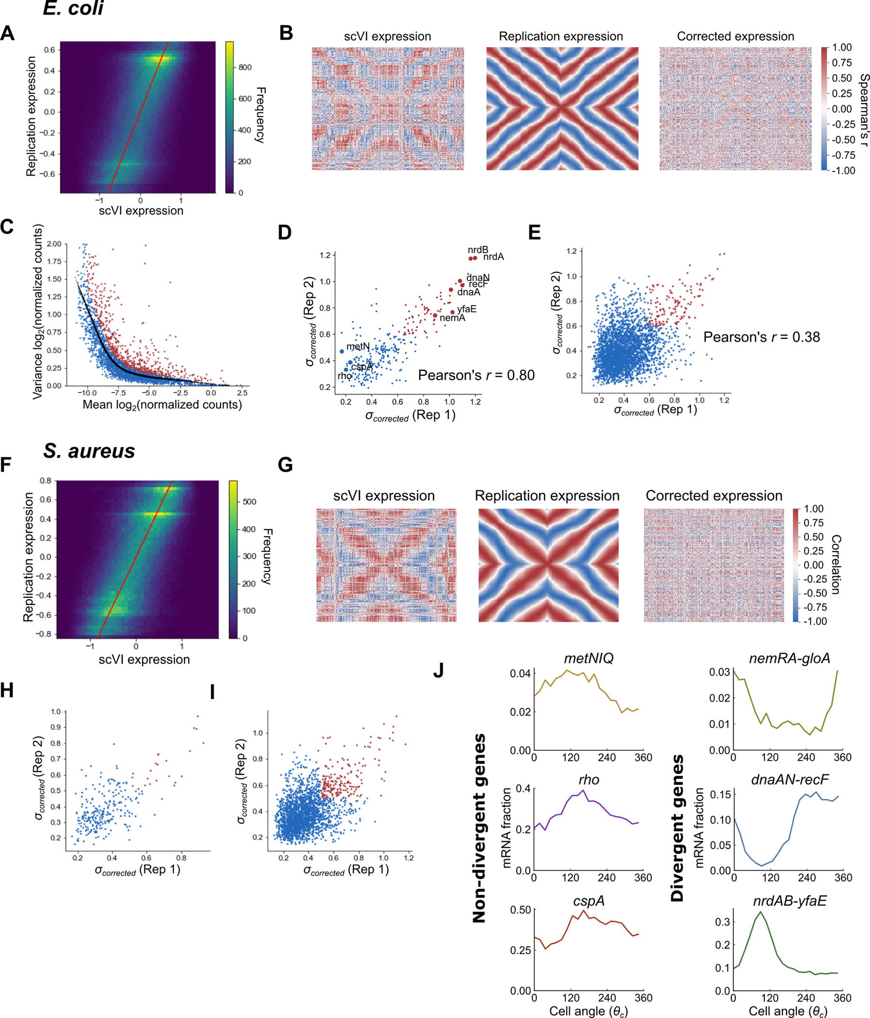
A) Two-dimensional histogram for E. coli showing the relationship between observed expression from scVI and replication-predicted expression. Expression is averaged in 100 bins by cell angle ${\theta }_c$. The red line indicates x = y i.e. the case where expression in both matrices is identical. Overall, there is a rough 1:1 correspondence between observed and predicted expression, indicating a good model fit (Pearson’s r = 0.59). B) Gene-gene correlations in LB-grown E. coli across ${\theta }_c$-binned expression data (100 bins) for the full scVI observed model (left), the replication-only model (middle), and the corrected model that is the difference of the two expression matrices (right). C) The mean-variance relationship in E. coli of log-transformed normalized counts. The black line indicates the locally weighted scatterplot smoothing (LOWESS)-fitted values and red points are genes classed as highly variable. See Methods for further details. D) Comparison of the divergence score ${\sigma }_{\mathit{corrected}}$ between LB-grown E. coli in Datasets D1 & D2 of genes classed as highly variable in both datasets (287 genes). Red indicates replication-divergent genes (${\sigma }_{\mathit{corrected}}>0.6$). E) Comparison of ${\sigma }_{\mathit{corrected}}$ (standard deviation of divergence from the replication model) between LB-grown E. coli in Dataset D1 and Dataset D2 of all genes present in both datasets. Red indicates ${\sigma }_{\mathit{corrected}}>0.6$ in both datasets, meaning that they are considered replication-divergent. F) Two-dimensional histogram as in (A) but for S. aureus. G) Gene-gene correlation plots as for (B) but for S. aureus (Pearson’s r = 0.67). H & I) Comparison of ${\sigma }_{\mathit{corrected}}$ (standard deviation of divergence from the replication model) between S. aureus in Dataset D5 and Dataset D6 for highly variable genes in both datasets (H) (Pearson’s r = 0.66) and all genes (I) (Pearson’s r = 0.48). Red indicates ${\sigma }_{\mathit{corrected}}>0.5$ in both datasets, meaning that they are considered replication-divergent. J) Gene expression plots of select genes based on unsmoothed counts. Raw counts were normalized by total UMI/cell and then averaged in 20 bins by cell angle ${\theta }_c$. Expression was averaged across genes within each operon.

Extended Data Fig. 5: smFISH analysis of cell cycle gene expression correlates with phase-shifted scRNA-seq data.

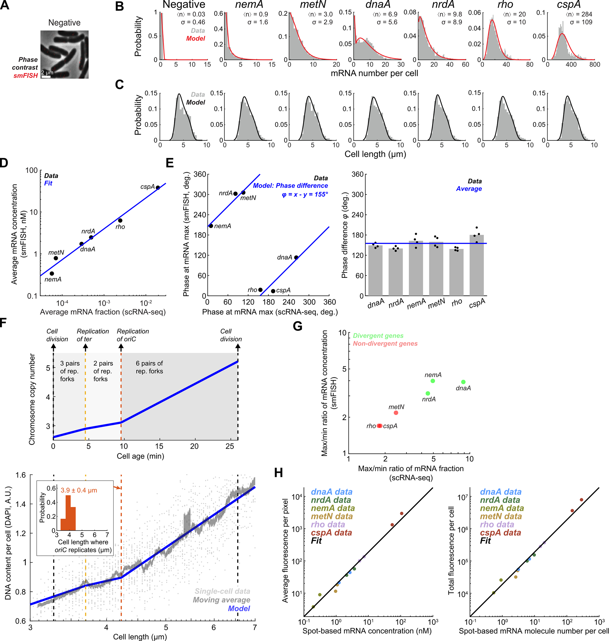
A) Negative control for smFISH labeling. E. coli cells labeled against bacteriophage lambda cI mRNA. smFISH signal is shown using the same contrast as in Fig. 2I & Extended Data Fig. 6A. Representative of two independent experiments. See SI Methods Section “Oligonucleotide probe design”. B) The distribution of mRNA copy-number per cell for each gene. See SI Methods Section “mRNA quantification”. Red line, fit to a negative binomial distribution plus a “zero spike”. C) The distribution of cell length in each sample. Black line, fit to the theoretical model, see SI Methods Section “Modeling the distribution of cell length”. D) Comparison of the population-averaged mRNA fraction, as measured using scRNA-seq, with mRNA concentration, as measured using smFISH. Markers indicate averages of two biological replicates by each method. Blue line, fit to a function y = ax^b. E) Estimation of the cell-cycle phase difference between scRNA-seq and smFISH. The phase of each dataset was estimated as described in SI Methods Section “Cell-cycle analysis of mRNA concentration”. Left: markers indicate averages of two biological replicates by each method. Blue line, fit to a linear function, indicating a constant phase difference φ. Right: the estimated phase difference across the six genes examined. The bars represent the average of four pairwise differences calculated from two biological replicates of each method. F) Top: the theoretically predicted cellular DNA contents as a function of cell age, see SI Methods Section “Inferring cell-cycle phase from the DAPI signal”. Bottom: DAPI-measured DNA content per cell as a function of cell length. Single-cell data was binned based on cell length (moving average ± SEM, 21 cells per bin), Blue line, fit to the theoretical model. Inset, the distribution of the inferred cell length where oriC replicates, estimated from all smFISH samples. G) Divergent genes exhibit a larger amplitude of cell-cycle fluctuations. The ratio between the maximum and minimum expression level of different genes, as measured using scRNA-seq and smFISH. The mRNA fraction (scRNA-seq) and concentration (smFISH) were obtained as in Fig. 2I & Extended Data Fig. 6A, 2nd and 3rd columns. The maximum and minimum levels were determined from the binned data. Markers indicate averages of two biological replicates by each method. H) Consistency between spot-based and cell-based smFISH quantification. Comparison of the mRNA levels inferred from smFISH data using spot-based and cell-based mRNA quantification. Both methods are described in SI Methods Section “mRNA quantification”. Left: mRNA concentration. Right: mRNA copy number per cell. Markers indicate mean values from each smFISH sample. Black line, fit to a linear function.

Extended Data Fig. 6: Cell cycle analysis of smFISH and scRNA-seq shows good agreement across biological replicates.

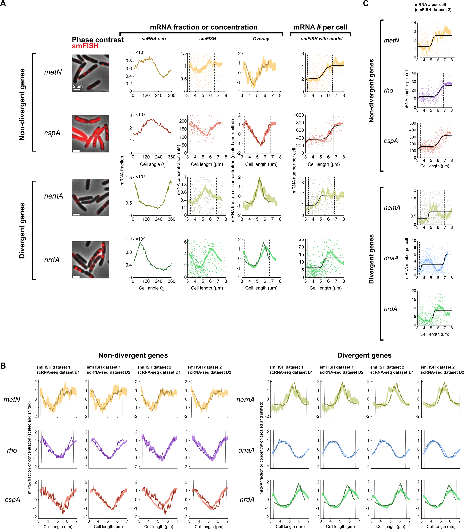
A) Comparison between scRNA-seq and smFISH with relative and absolute expression, as in Fig. 2I but for other genes shown in Fig. 2H. From left to right: 1) Microscopy images of E. coli cells labeled using smFISH against the indicated gene (cspA is visualized with alternative contrast, for negative control see Extended Data Fig. 5A); 2) scRNA-seq expression shown as fraction of total cellular mRNA (expression is averaged in 100 bins by ${\theta }_c$); 3) mRNA concentration, measured using smFISH, as a function of cell length. Single-cell data (scatter plot) was binned by cell length (shaded curve, moving average ± SEM, 10% sample size per bin). Dashed lines indicate the twofold length range where most cells reside, used to infer the mean values at birth and division; 4) Alignment of scaled data from smFISH and scRNA-seq measurements; 5) Absolute mRNA copy number, measured using smFISH, as a function of cell length. Single-cell data was processed as in column 3 (5% sample size per bin). Black line, fit to a sum of two Hill functions, corresponding to two gene replication rounds. B) Pairwise comparison between two smFISH and two scRNA-seq datasets. Analysis as in Fig. Fig. 2I & (A), 4th column. See SI Methods Section “mRNA quantification”. C) Absolute mRNA copy number, measured using smFISH, as a function of cell length. Displayed as for Fig. 2I & (A), column (5), but for smFISH replicate 2.

Extended Data Fig. 7: The relationship between distance from the transcriptional start site and gene expression timing and amplitude.

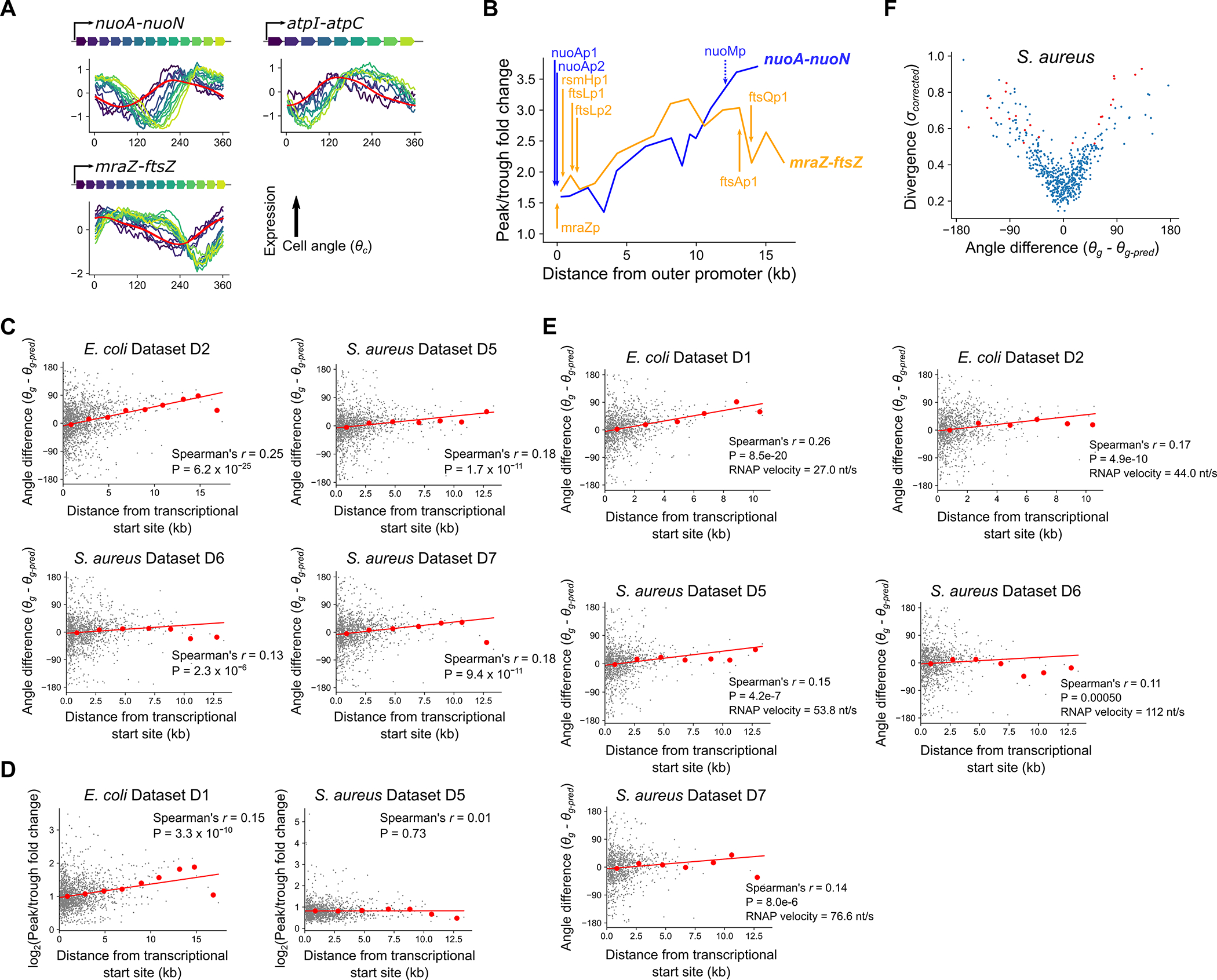
A) Cell cycle gene expression plots for operons showing “delayed” genes as in Fig. 3B but for LB-grown WT E. coli from Dataset D2. The red line indicates predicted expression. B) Amplitude measured as peak/trough fold change (SI Methods Section “Identifying genes with high divergence from predicted expression”) as a function of distance from the promoter for two large operons, nuoA->nuoN and mraZ->ftsZ. The positions of promoters on each operon are marked by arrows. All are supported by direct experimental evidence (evidence code ‘EV-EXP-IDA’) except for nuoMp (dotted arrow), which is inferred from expression pattern only (evidence code ‘EV-EXP-IEP’). For a description of the evidence ontology, see http://brg.ai.sri.com/evidence-ontology/downloads/evidence.html. C) Plots of maximum distance from a transcriptional start site against difference between predicted and observed angles as in Fig. 3C. Red line indicates the linear model fit and red points indicate averages of 2 kb bins. Data are shown for additional E. coli replicates and all S. aureus replicates. P-values are based on a two-sided statistical test with the null hypothesis of no correlation. See Methods for details. D) Plots as in (C) but of maximum distance from a transcriptional start site against the log₂-transformed peak/trough ratio in gene expression, calculated as described in SI Methods Section “Identifying genes with high divergence from predicted expression”. E) Plots as in (C) but using manual operon annotation. Here, any tandem, contiguous stretch of genes with an intergenic distance less than 40 bp is considered an operon. Transcriptional start sites are defined as the start position of the first gene in the operon. F) Plot of divergence from predictions against the difference between predicted and observed angles, as in Fig. 3A but for S. aureus.

Extended Data Fig. 8: Cell cycle analysis of the B. subtilis transcriptome.

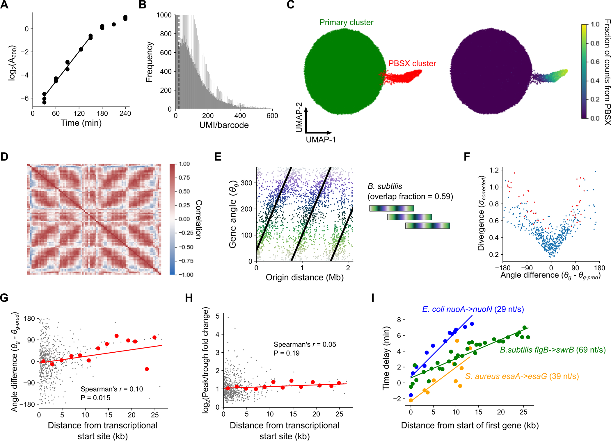
A) Growth curve of B. subtilis in LB. Black line indicates linear portion used to calculate growth rate. Data shown are from four biological replicates. B) UMI per barcode distribution for B. subtilis (Dataset D9 Rep 1). Axes have been clipped for visualization purposes. The dashed black line indicates the minimum threshold of 20 UMI/barcode for this sample. C) Presence of an additional cluster associated with PBSX prophage mobilization. Left: UMAP visualization of initial clustering in B. subtilis. UMAP was performed on the latent space representation generated by scVI²². Red indicates a cluster driven by PBSX mobilization that was excluded from downstream analyses. Green is the cluster used for downstream analysis. Leiden clustering was performed using scanpy. Right: Same UMAP visualization but represented as the fraction of mRNA counts mapping to the PBSX prophage (based on annotation from phaster.ca). Note that 1.5% of cells contain at least three transcripts mapping to this prophage. D) Chromosome-wide correlation of gene expression in 50 kb bins as in Fig. 1C. Analysis was performed after the PBSX cluster was removed. E) Origin distance-gene angle relationship as in Fig. 2E. Overlap between rounds of replications is visualized as in Fig. 2G. F) Relationship between angle difference and divergence from predictions for all highly variable genes. As in Fig. 3A. G) Relationship between angle difference and distance from the transcriptional start site as in Fig. 3C. Spearman correlation and significance of the relationship are shown. P-values are based on a two-sided statistical test with the null hypothesis of no correlation. See Methods for details. H) Relationship between expression amplitude (peak/trough fold change) and distance from the transcriptional start site as in Extended Data Fig. 7D. Spearman correlation and significance of the relationship are shown. P-values are based on a two-sided statistical test with the null hypothesis of no correlation. See Methods for details. I) Comparison between long operons from different species. Angle difference is converted to “Time delay” by dividing by 360° and multiplying by the doubling time in minutes, allowing standardization across species. Distance is measured as distance of the first base position of each gene in the operon from the first base position of the first gene in the operon. Inferred RNAP speeds from linear model fits to the individual operons are shown.

Extended Data Fig. 9: Transcription-replication interactions in E. coli and S. aureus.

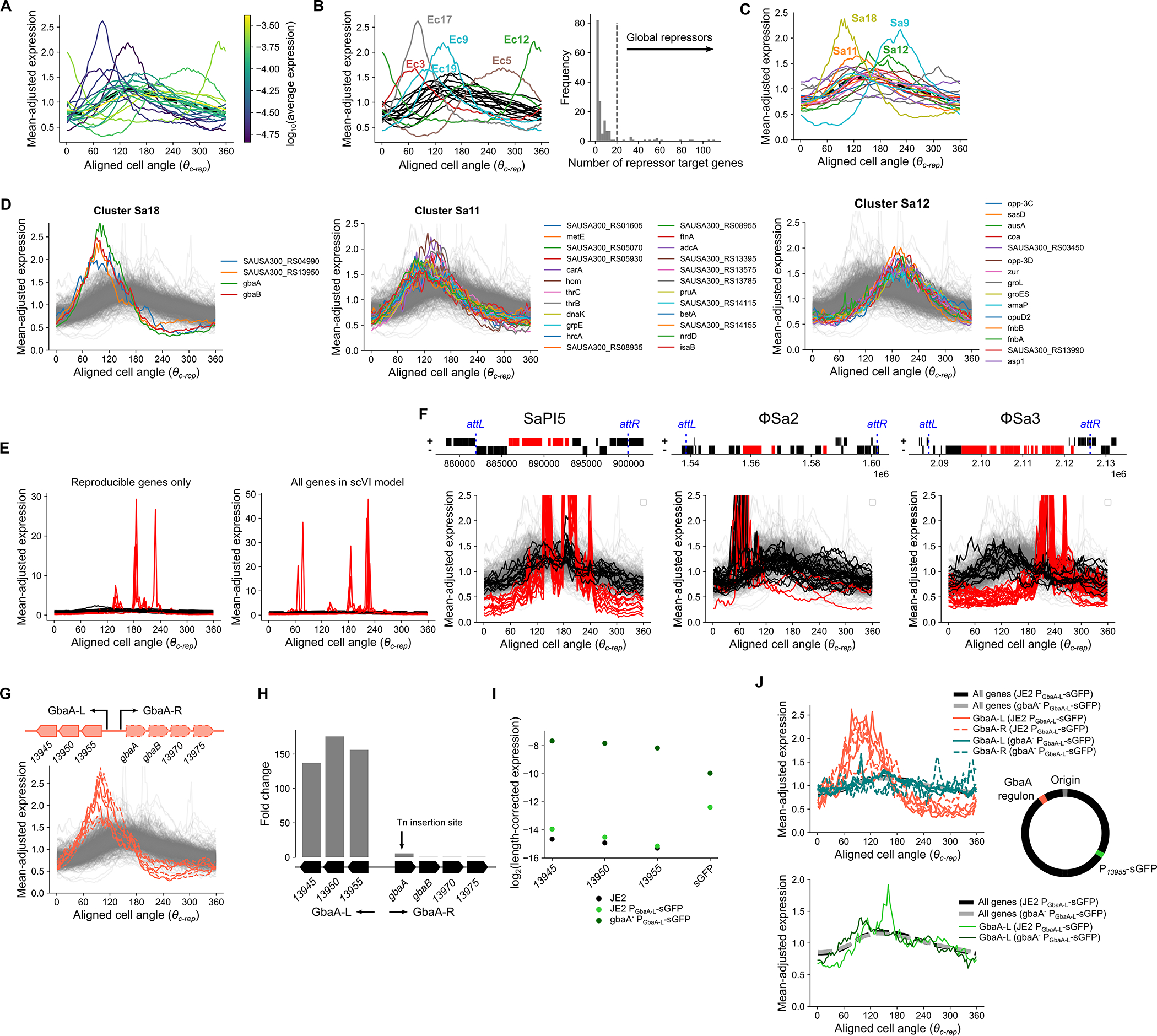
A) Clusters as in Fig. 4B but colored according to their average, length-corrected expression. This was determined by a gene’s mean fraction of total mRNA that was length-corrected by dividing by its length and multiplying by the median gene length across genes. B) Left: Clusters as in Fig. 4B but with coloring only for those clusters that are enriched for repressed genes (FDR = 0.1, hypergeometric test) colored. Non-significant clusters are in black. Right: Histogram of the number of annotated repressor targets by transcription factor. Those with 20 or more target genes were excluded from the hypergeometric analysis. See Methods Section “Clustering of TRIPs” for further details. C) Plot as in Fig. 4B except for mean expression of S. aureus clusters. Genes situated on mobile genetic elements were removed prior to clustering analysis. D) Plots of individual genes from clusters indicated in (C). E) Mean cluster expression of TRIPs partitioned into 20 clusters by aligned gene expression $\left({\theta }_{c-rep}\right)$. Clusters in red are those that only contain genes located within MGEs. Left: Reproducible genes; Right: all genes included in the scVI model (regardless of reproducibility). The cluster assignments on the right are used for (F). F) Expression of genes within mobile elements. Genes are colored based on whether they are in MGE-exclusive clusters from (E) (Right panel) (red) or other clusters (black). Top: schematic figure of MGE gene content. The x-axis represents chromosomal coordinate and + and − strands are plotted separately by y-axis position. Predicted attachment sites attL and attR denote the predicted boundaries of the MGE and are annotated in blue. Annotation for MGEs was taken from the online tool Phaster. Bottom: Plots of MGE genes by aligned gene expression $\left({\theta }_{c-rep}\right)$ as represented in Fig. 4. Gray genes represent the non-MGE background. Note that phage ΦSa2 is disabled and expression of its MGE-specific (“red”) cluster genes is low (0.002% of cells contain at least three transcripts) compared to the staphylococcal pathogenicity island (SaPI) 5 (0.4%) and phage ΦSa3 (0.07%), potentially contributing to the less clear delineation between expression profiles by gene type. MGE-specific expression patterns may arise due to MGE mobilization and these patterns may represent rare events that are not effectively captured by our cell cycle analysis, meaning that the plots here should be interpreted with caution. G) Aligned expression profiles for genes within the GbaA regulon for USA300 LAC WT. Plotted as in Fig. 4D, with mean-adjusted expression shown and all other reproducible genes shown in gray. The structure of the regulon is shown as a schematic figure above. H) Expression fold change of genes in the GbaA regulon after gbaA transposon insertion. Genes of the GbaA-L operon increase in expression >100–fold. However, due to the location of the transposon insertion towards the 5’ end of gbaA, induction of GbaA-R genes is not observed. Genes with names starting with SAUSA300_RS are truncated to give only the unique number. I) Average expression of GbaA-L genes and sGFP in reporter strains (compared to JE2 in measurements from the same experiment). Average expression measured as fraction of total mRNA was length-corrected as elsewhere by dividing by the gene length and multiplying by the median gene length across all genes. Note that sGFP expression in JE2 P_GbaA-L-sGFP is approximately fourfold higher than that of GbaA-L genes, and the derepressed form in gbaA⁻ P_GbaA-L-sGFP is also fourfold lower (possibly reflecting lower copy number due to its further distance from the origin). Therefore, while repression of the GbaA-L locus is ~96-fold, repression of sGFP by GbaA is only 5.3-fold. J) Comparison of aligned expression $\left({\theta }_{c-rep}\right)$ (as in Fig. 4) for GbaA regulon genes and sGFP in the two reporter constructs. Thick black and gray lines represent average expression across all reproducible genes. The schematic figure represents the relative positions of the GbaA regulon and the P_GbaA-L-sGFP integration site.

Extended Data Fig. 10: Biophysical modeling of cell cycle gene expression dynamics.

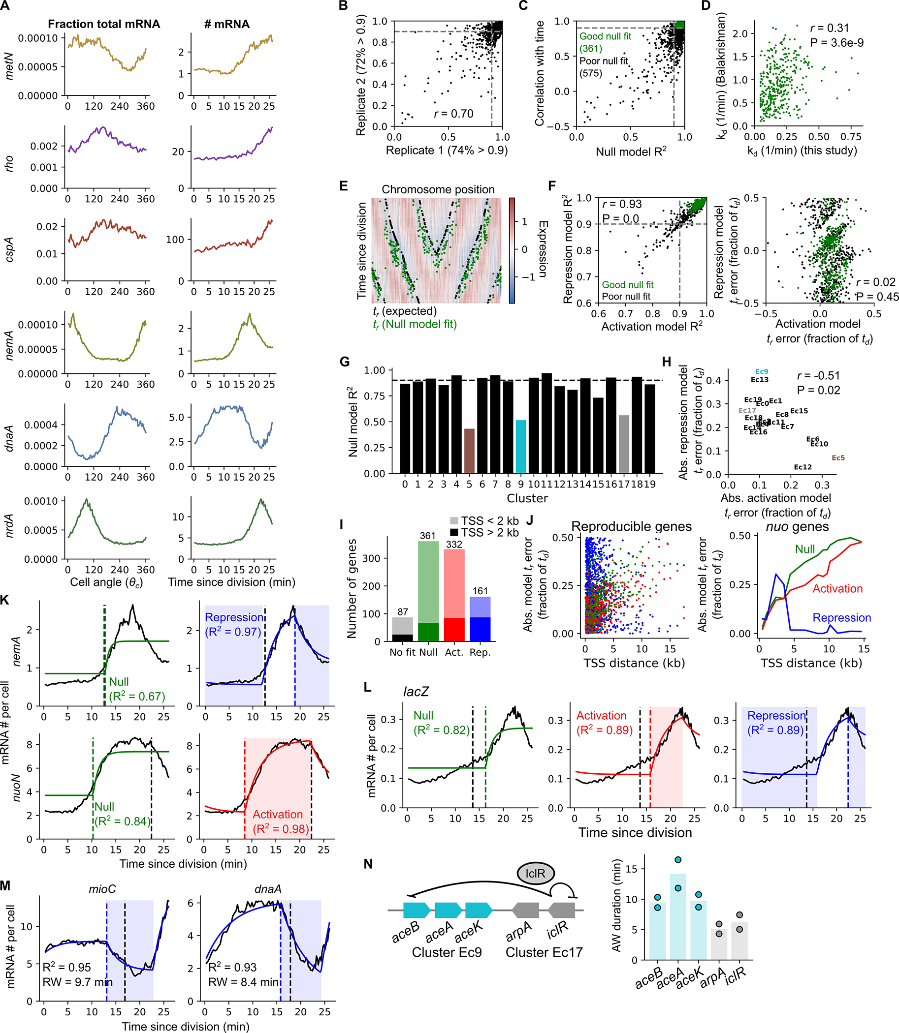
A) Conversion from fraction of total mRNA per cell as a function of cell angle to the estimated absolute number of mRNA per cell as a function of time since cell division. Data are shown for the individual genes displayed in Fig. 2I & Extended Data Fig. 6A. B) R² values for all reproducible genes (correlation between replicates >0.7) from fitting to the null model, compared between the two replicates for E. coli grown in LB. The Spearman correlation between the two replicates is shown. Grey dashed lines indicate R² = 0.9, which we use as a threshold for good fit with the data. C) In order to assess fit to the null model, we rely on an additional assumption that gene dosage-driven expression values should increase monotonically within the cell cycle. To evaluate monotonicity, we calculate the Spearman correlation between number of mRNA per cell and time. Genes that have both a good fit to the model (R² > 0.9) and good monotonicity with time (Spearman’s r > 0.9) are considered null model genes as indicated in green and quantified in (I). D) Comparison of degradation rates (k_d) for all genes with a good fit to the null model between fitted values in this study and those inferred from rapamycin responses in Balakrishnan et al. Data are from Dataset D1 but are representative of two independent biological experiments (also Dataset D2). E) Fitted and expected replication times and their relation to gene expression. A heatmap is shown for scaled expression as a function of time and chromosome position (similar to Fig. 2B). Superimposed on this are expected replication times ($t_r$) of the null model genes, based on predicted expression minima (black dots) (Methods Section “Defining gene Transcription-Replication Interaction Profiles (TRIPs)“) or based on fits to the null model (green dots) (SI Methods Section “The null model”). F) Comparing fits between activation and repression models. These models have more parameters than the null model and this flexibility means they tend to give very good fits based on R². Since R² values are highly correlated between models (left panel), this limits the usefulness of R² to distinguish between gene profiles. By contrast, the ability of the models to infer accurately the predicted replication time, $t_r$, differs greatly between models, with no correlation between the errors in each model for fitted $t_r$ compared to expectations (right panel). Data are from Dataset D1 but are representative of two independent biological experiments (also Dataset D2). G) Average null model fit (R²) for clusters defined in Fig. 4B. Key clusters are highlighted by their colors in Fig. 4B. Note that for activation and repression models, all clusters have average R² > 0.9. H) Absolute values of errors in prediction of replication timing $t_r$ as a fraction of $t_d$, averaged across Fig. 4B clusters. Values for activation and repression models are compared. Error in fitted $t_r$ compared to $t_r$ based on the predicted expression minimum was calculated as in (E) for activation and repression models. Absolute values of these errors were averaged across genes within each cluster. There is a significant negative correlation between these, implying that replication timings of clusters well-predicted by the activation model are poorly predicted by the repression model and vice versa. Highlighted clusters are colored as in Fig. 4B. Data are from Dataset D1 but are representative of two independent biological experiments (also Dataset D2). I) Number of genes among reproducible genes that are well-fit by either null, activation, or repression models (or no good fit to any). See Methods for decision criteria used. For each one, the portion of genes whose midpoint is >2 kb from the transcriptional start site (TSS) is indicated. Only the repression model is enriched for genes >2 kb from their TSS (hypergeometric test, P = 5e-15, compared to P > 0.4 for all other models). J) Absolute values of error in prediction of $t_r$ (as a fraction of $t_d$) for all three models as a function of distance from the TSS for all genes (left panel) or genes within the nuo operon (right panel). K) Alternative model fits for genes fitting the activation (nemA) or repression (nuoN) models. For these genes, the null model can be rejected because of the poor R², whereas the repression or activation models can be rejected for nemA and nuoN, respectively, because of their poor prediction of $t_r$ (see Fig. 5 for comparison). L) Expression profiles and model fits for the lacZ gene. Note that while the fit of lacZ is imperfect to any model (possibly due to its very low expression under these conditions, which reduces data quality), the activation model does the best when both R² and prediction of $t_r$ are considered. M) Additional plots for two genes with good fits to the repression model. N) Expression dynamics of genes in the IclR regulon. IclR is encoded by iclR and is adjacent to the aceBAK operon. IclR represses its own transcription as well as that of the nearby aceBAK operon. Regulation of the gene arpA is not described but it is downstream of iclR. arpA is annotated as belonging to a single gene transcript, but the similar expression patterns suggest that it may actually share an operon with iclR. All genes fit to the activation model, however iclR and arpA exhibit early heterochrony (Ec17, Class 2a, Fig. 4C) whereas aceBAK does not (Ec9, Class 2b, Fig. 4D). The activation model fit predicts a shorter window of activation (right panel) in iclR/arpA compared to aceBAK. The bar plot represents the mean activation window duration with points representing the values of individual replicates.

Data availability

All counts matrices and raw sequencing reads used to perform the scRNA-seq analysis are available in the Gene Expression Omnibus (GEO) under the accession number GSE217715. Previously published counts matrices used for bulk analysis of C. crescentus expression are available in GEO under the accession number GSE46915.

References

- 1.Bervoets I & Charlier D Diversity, versatility and complexity of bacterial gene regulation mechanisms: opportunities and drawbacks for applications in synthetic biology. FEMS Microbiol. Rev. 43, 304–339 (2019). [DOI] [PMC free article] [PubMed] [Google Scholar]
- 2.Vilar JMG, Guet CC & Leibler S Modeling network dynamics: the lac operon, a case study. J. Cell Biol. 161, 471–476 (2003). [DOI] [PMC free article] [PubMed] [Google Scholar]
- 3.Narula J, Devi SN, Fujita M & Igoshin OA Ultrasensitivity of the Bacillus subtilis sporulation decision. Proc. Natl. Acad. Sci. U. S. A. 109, E3513–22 (2012). [DOI] [PMC free article] [PubMed] [Google Scholar]
- 4.Homberger C, Hayward RJ, Barquist L & Vogel J Improved bacterial single-cell RNA-seq through automated MATQ-seq and Cas9-based removal of rRNA reads. Preprint at 10.1101/2022.11.28.518171. [DOI] [PMC free article] [PubMed]
- 5.Balakrishnan R et al. Principles of gene regulation quantitatively connect DNA to RNA and proteins in bacteria. Science 378, eabk2066 (2022). [DOI] [PMC free article] [PubMed] [Google Scholar]
- 6.Cooper S & Helmstetter CE Chromosome replication and the division cycle of Escherichia coli B/r. J. Mol. Biol. 31, 519–540 (1968). [DOI] [PubMed] [Google Scholar]
- 7.Schaechter M, Bentzon MW & Maaloe O Synthesis of deoxyribonucleic acid during the division cycle of bacteria. Nature 183, 1207–1208 (1959). [DOI] [PubMed] [Google Scholar]
- 8.Wang M, Zhang J, Xu H & Golding I Measuring transcription at a single gene copy reveals hidden drivers of bacterial individuality. Nat Microbiol 4, 2118–2127 (2019). [DOI] [PMC free article] [PubMed] [Google Scholar]
- 9.Narula J et al. Chromosomal Arrangement of Phosphorelay Genes Couples Sporulation and DNA Replication. Cell 162, 328–337 (2015). [DOI] [PMC free article] [PubMed] [Google Scholar]
- 10.Slager J & Veening J-W Hard-Wired Control of Bacterial Processes by Chromosomal Gene Location. Trends Microbiol. 24, 788–800 (2016). [DOI] [PMC free article] [PubMed] [Google Scholar]
- 11.Peterson JR, Cole JA, Fei J, Ha T & Luthey-Schulten ZA Effects of DNA replication on mRNA noise. Proc. Natl. Acad. Sci. U. S. A. 112, 15886–15891 (2015). [DOI] [PMC free article] [PubMed] [Google Scholar]
- 12.Laub MT, McAdams HH, Feldblyum T, Fraser CM & Shapiro L Global analysis of the genetic network controlling a bacterial cell cycle. Science 290, 2144–2148 (2000). [DOI] [PubMed] [Google Scholar]
- 13.Fang G et al. Transcriptomic and phylogenetic analysis of a bacterial cell cycle reveals strong associations between gene co-expression and evolution. BMC Genomics 14, 450 (2013). [DOI] [PMC free article] [PubMed] [Google Scholar]
- 14.Zhou B et al. The global regulatory architecture of transcription during the Caulobacter cell cycle. PLoS Genet. 11, e1004831 (2015). [DOI] [PMC free article] [PubMed] [Google Scholar]
- 15.De Nisco NJ, Abo RP, Wu CM, Penterman J & Walker GC Global analysis of cell cycle gene expression of the legume symbiont Sinorhizobium meliloti. Proc. Natl. Acad. Sci. U. S. A. 111, 3217–3224 (2014). [DOI] [PMC free article] [PubMed] [Google Scholar]
- 16.Bandekar AC, Subedi S, Ioerger TR & Sassetti CM Cell-Cycle-Associated Expression Patterns Predict Gene Function in Mycobacteria. Curr. Biol. 30, 3961–3971.e6 (2020). [DOI] [PMC free article] [PubMed] [Google Scholar]
- 17.Cooper S The synchronization manifesto: a critique of whole-culture synchronization. FEBS J. 286, 4650–4656 (2019). [DOI] [PubMed] [Google Scholar]
- 18.Blattman SB, Jiang W, Oikonomou P & Tavazoie S Prokaryotic single-cell RNA sequencing by in situ combinatorial indexing. Nat Microbiol 5, 1192–1201 (2020). [DOI] [PMC free article] [PubMed] [Google Scholar]
- 19.Kuchina A et al. Microbial single-cell RNA sequencing by split-pool barcoding. Science 371, (2021). [DOI] [PMC free article] [PubMed] [Google Scholar]
- 20.Imdahl F, Vafadarnejad E, Homberger C, Saliba A-E & Vogel J Single-cell RNA-sequencing reports growth-condition-specific global transcriptomes of individual bacteria. Nat Microbiol 5, 1202–1206 (2020). [DOI] [PubMed] [Google Scholar]
- 21.Homberger C, Barquist L & Vogel J Ushering in a new era of single-cell transcriptomics in bacteria. microLife 3, (2022). [DOI] [PMC free article] [PubMed] [Google Scholar]
- 22.Lopez R, Regier J, Cole MB, Jordan MI & Yosef N Deep generative modeling for single-cell transcriptomics. Nat. Methods 15, 1053–1058 (2018). [DOI] [PMC free article] [PubMed] [Google Scholar]
- 23.Bremer H & Dennis PP Modulation of Chemical Composition and Other Parameters of the Cell at Different Exponential Growth Rates. EcoSal Plus 3, (2008). [DOI] [PubMed] [Google Scholar]
- 24.Michelsen O, Teixeira de Mattos MJ, Jensen PR & Hansen FG Precise determinations of C and D periods by flow cytometry in Escherichia coli K-12 and B/r. Microbiology 149, 1001–1010 (2003). [DOI] [PubMed] [Google Scholar]
- 25.Wang X, Lesterlin C, Reyes-Lamothe R, Ball G & Sherratt DJ Replication and segregation of an Escherichia coli chromosome with two replication origins. Proc. Natl. Acad. Sci. U. S. A. 108, E243–50 (2011). [DOI] [PMC free article] [PubMed] [Google Scholar]
- 26.Dimude JU et al. Origins Left, Right, and Centre: Increasing the Number of Initiation Sites in the Chromosome. Genes 9, (2018). [DOI] [PMC free article] [PubMed] [Google Scholar]
- 27.Ivanova D et al. Shaping the landscape of the Escherichia coli chromosome: replication-transcription encounters in cells with an ectopic replication origin. Nucleic Acids Res. 43, 7865–7877 (2015). [DOI] [PMC free article] [PubMed] [Google Scholar]
- 28.Khodursky AB et al. Analysis of topoisomerase function in bacterial replication fork movement: use of DNA microarrays. Proc. Natl. Acad. Sci. U. S. A. 97, 9419–9424 (2000). [DOI] [PMC free article] [PubMed] [Google Scholar]
- 29.Pham TM et al. A single-molecule approach to DNA replication in Escherichia coli cells demonstrated that DNA polymerase III is a major determinant of fork speed. Mol. Microbiol. 90, 584–596 (2013). [DOI] [PubMed] [Google Scholar]
- 30.Kjeldgaard NO, Maaloe O & Schaechter M The transition between different physiological states during balanced growth of Salmonella typhimurium. J. Gen. Microbiol. 19, 607–616 (1958). [DOI] [PubMed] [Google Scholar]
- 31.Skinner SO, Sepúlveda LA, Xu H & Golding I Measuring mRNA copy number in individual Escherichia coli cells using single-molecule fluorescent in situ hybridization. Nat. Protoc. 8, 1100–1113 (2013). [DOI] [PMC free article] [PubMed] [Google Scholar]
- 32.Proshkin S, Rahmouni AR, Mironov A & Nudler E Cooperation between translating ribosomes and RNA polymerase in transcription elongation. Science 328, 504–508 (2010). [DOI] [PMC free article] [PubMed] [Google Scholar]
- 33.Pomerantz RT & O’Donnell M The replisome uses mRNA as a primer after colliding with RNA polymerase. Nature 456, 762–766 (2008). [DOI] [PMC free article] [PubMed] [Google Scholar]
- 34.de la Fuente A, Palacios P & Vicente M Transcription of the Escherichia coli dcw cluster: evidence for distal upstream transcripts being involved in the expression of the downstream ftsZ gene. Biochimie 83, 109–115 (2001). [DOI] [PubMed] [Google Scholar]
- 35.Flärdh K, Palacios P & Vicente M Cell division genes ftsQAZ in Escherichia coli require distant cis-acting signals upstream of ddlB for full expression. Mol. Microbiol. 30, 305–315 (1998). [DOI] [PubMed] [Google Scholar]
- 36.Lutkenhaus JF, Wolf-Watz H & Donachie WD Organization of genes in the ftsA-envA region of the Escherichia coli genetic map and identification of a new fts locus (ftsZ). J. Bacteriol. 142, 615–620 (1980). [DOI] [PMC free article] [PubMed] [Google Scholar]
- 37.Zaslaver A, Mayo A, Ronen M & Alon U Optimal gene partition into operons correlates with gene functional order. Phys. Biol. 3, 183–189 (2006). [DOI] [PubMed] [Google Scholar]
- 38.Zhu M, Mu H, Han F, Wang Q & Dai X Quantitative analysis of asynchronous transcription-translation and transcription processivity in under various growth conditions. iScience 24, 103333 (2021). [DOI] [PMC free article] [PubMed] [Google Scholar]
- 39.Zhu M, Mori M, Hwa T & Dai X Disruption of transcription-translation coordination in Escherichia coli leads to premature transcriptional termination. Nat Microbiol 4, 2347–2356 (2019). [DOI] [PMC free article] [PubMed] [Google Scholar]
- 40.Sharpe ME, Hauser PM, Sharpe RG & Errington J Bacillus subtilis cell cycle as studied by fluorescence microscopy: constancy of cell length at initiation of DNA replication and evidence for active nucleoid partitioning. J. Bacteriol. 180, 547–555 (1998). [DOI] [PMC free article] [PubMed] [Google Scholar]
- 41.Golding I Revisiting Replication-Induced Transcription in Escherichia coli. Bioessays 42, e1900193 (2020). [DOI] [PMC free article] [PubMed] [Google Scholar]
- 42.Guptasarma P Does replication-induced transcription regulate synthesis of the myriad low copy number proteins of Escherichia coli? Bioessays 17, 987–997 (1995). [DOI] [PubMed] [Google Scholar]
- 43.Ray A, Edmonds KA, Palmer LD, Skaar EP & Giedroc DP Glucose-Induced Biofilm Accessory Protein A (GbaA) Is a Monothiol-Dependent Electrophile Sensor. Biochemistry 59, 2882–2895 (2020). [DOI] [PMC free article] [PubMed] [Google Scholar]
- 44.Van Loi V et al. The two-Cys-type TetR repressor GbaA confers resistance under disulfide and electrophile stress in Staphylococcus aureus. Free Radic. Biol. Med. 177, 120–131 (2021). [DOI] [PMC free article] [PubMed] [Google Scholar]
- 45.Campbell JL & Kleckner NE coli oriC and the dnaA gene promoter are sequestered from dam methyltransferase following the passage of the chromosomal replication fork. Cell 62, 967–979 (1990). [DOI] [PubMed] [Google Scholar]
- 46.Theisen PW, Grimwade JE, Leonard AC, Bogan JA & Helmstetter CE Correlation of gene transcription with the time of initiation of chromosome replication in Escherichia coli. Mol. Microbiol. 10, 575–584 (1993). [DOI] [PubMed] [Google Scholar]
- 47.Buettner F et al. Computational analysis of cell-to-cell heterogeneity in single-cell RNA-sequencing data reveals hidden subpopulations of cells. Nat. Biotechnol. 33, 155–160 (2015). [DOI] [PubMed] [Google Scholar]
- 48.Cooper S The Escherichia coli cell cycle. Res. Microbiol. 141, 17–29 (1990). [DOI] [PubMed] [Google Scholar]
- 49.Garrido T, Sánchez M, Palacios P, Aldea M & Vicente M Transcription of ftsZ oscillates during the cell cycle of Escherichia coli. EMBO J. 12, 3957–3965 (1993). [DOI] [PMC free article] [PubMed] [Google Scholar]
- 50.Zhou P & Helmstetter CE Relationship between ftsZ gene expression and chromosome replication in Escherichia coli. J. Bacteriol. 176, 6100–6106 (1994). [DOI] [PMC free article] [PubMed] [Google Scholar]
- 51.Lin J & Amir A Homeostasis of protein and mRNA concentrations in growing cells. Nat. Commun. 9, 4496 (2018). [DOI] [PMC free article] [PubMed] [Google Scholar]
- 52.Rosenfeld N, Elowitz MB & Alon U Negative autoregulation speeds the response times of transcription networks. J. Mol. Biol. 323, 785–793 (2002). [DOI] [PubMed] [Google Scholar]
- 53.Ma P et al. Bacterial droplet-based single-cell RNA-seq reveals antibiotic-associated heterogeneous cellular states. Cell 186, 877–891.e14 (2023). [DOI] [PMC free article] [PubMed] [Google Scholar]
- 54.Brennan MA & Rosenthal AZ Single-Cell RNA Sequencing Elucidates the Structure and Organization of Microbial Communities. Front. Microbiol. 12, 713128 (2021). [DOI] [PMC free article] [PubMed] [Google Scholar]
- 55.Xu Z et al. Droplet-based high-throughput single microbe RNA sequencing by smRandom-seq. Nat. Commun. 14, 5130 (2023). [DOI] [PMC free article] [PubMed] [Google Scholar]
- 56.Luecken MD & Theis FJ Current best practices in single-cell RNA-seq analysis: a tutorial. Mol. Syst. Biol. 15, e8746 (2019). [DOI] [PMC free article] [PubMed] [Google Scholar]
- 57.Jun S, Si F, Pugatch R & Scott M Fundamental principles in bacterial physiology-history, recent progress, and the future with focus on cell size control: a review. Rep. Prog. Phys. 81, 056601 (2018). [DOI] [PMC free article] [PubMed] [Google Scholar]
- 58.La Manno G et al. RNA velocity of single cells. Nature 560, 494–498 (2018). [DOI] [PMC free article] [PubMed] [Google Scholar]
- 59.Bergen V, Soldatov RA, Kharchenko PV & Theis FJ RNA velocity-current challenges and future perspectives. Mol. Syst. Biol. 17, e10282 (2021). [DOI] [PMC free article] [PubMed] [Google Scholar]
Additional references
- 60.Wolf FA, Angerer P & Theis FJ SCANPY: large-scale single-cell gene expression data analysis. Genome Biol. 19, 15 (2018). [DOI] [PMC free article] [PubMed] [Google Scholar]
- 61.Arndt D et al. PHASTER: a better, faster version of the PHAST phage search tool. Nucleic Acids Res. 44, W16–21 (2016). [DOI] [PMC free article] [PubMed] [Google Scholar]
- 62.Levin M et al. The mid-developmental transition and the evolution of animal body plans. Nature 531, 637–641 (2016). [DOI] [PMC free article] [PubMed] [Google Scholar]
- 63.Zalts H & Yanai I Developmental constraints shape the evolution of the nematode mid-developmental transition. Nat Ecol Evol 1, 113 (2017). [DOI] [PubMed] [Google Scholar]
- 64.Keseler IM et al. The EcoCyc Database in 2021. Front. Microbiol. 12, 711077 (2021). [DOI] [PMC free article] [PubMed] [Google Scholar]
- 65.Karp PD et al. The BioCyc collection of microbial genomes and metabolic pathways. Brief. Bioinform. 20, 1085–1093 (2019). [DOI] [PMC free article] [PubMed] [Google Scholar]
- 66.Fuchs S et al. AureoWiki-The repository of the Staphylococcus aureus research and annotation community. Int. J. Med. Microbiol. 308, 558–568 (2018). [DOI] [PubMed] [Google Scholar]
- 67.Virtanen P et al. SciPy 1.0: fundamental algorithms for scientific computing in Python. Nat. Methods 17, 261–272 (2020). [DOI] [PMC free article] [PubMed] [Google Scholar]
- 68.Love MI, Huber W & Anders S Moderated estimation of fold change and dispersion for RNA-seq data with DESeq2. Genome Biol. 15, 550 (2014). [DOI] [PMC free article] [PubMed] [Google Scholar]
- 69.Chen J, Yoong P, Ram G, Torres VJ & Novick RP Single-copy vectors for integration at the SaPI1 attachment site for Staphylococcus aureus. Plasmid 76, 1–7 (2014). [DOI] [PMC free article] [PubMed] [Google Scholar]
- 70.Benson MA et al. Staphylococcus aureus regulates the expression and production of the staphylococcal superantigen-like secreted proteins in a Rot-dependent manner. Mol. Microbiol. 81, 659–675 (2011). [DOI] [PMC free article] [PubMed] [Google Scholar]
- 71.Abdelhady W et al. Impact of vancomycin on sarA-mediated biofilm formation: role in persistent endovascular infections due to methicillin-resistant Staphylococcus aureus. J. Infect. Dis. 209, 1231–1240 (2014). [DOI] [PMC free article] [PubMed] [Google Scholar]
- 72.Kaneko H, Nakaminami H, Ozawa K, Wajima T & Noguchi N In vitro anti-biofilm effect of anti-methicillin-resistant Staphylococcus aureus (anti-MRSA) agents against the USA300 clone. J Glob Antimicrob Resist 24, 63–71 (2021). [DOI] [PubMed] [Google Scholar]
- 73.Kanehisa M & Goto S KEGG: kyoto encyclopedia of genes and genomes. Nucleic Acids Res. 28, 27–30 (2000). [DOI] [PMC free article] [PubMed] [Google Scholar]
- 74.Mootha VK et al. PGC-1alpha-responsive genes involved in oxidative phosphorylation are coordinately downregulated in human diabetes. Nat. Genet. 34, 267–273 (2003). [DOI] [PubMed] [Google Scholar]
- 75.Subramanian A et al. Gene set enrichment analysis: a knowledge-based approach for interpreting genome-wide expression profiles. Proc. Natl. Acad. Sci. U. S. A. 102, 15545–15550 (2005). [DOI] [PMC free article] [PubMed] [Google Scholar]
- 76.Fang Z, Liu X & Peltz G GSEApy: a comprehensive package for performing gene set enrichment analysis in Python. Bioinformatics 39, (2023). [DOI] [PMC free article] [PubMed] [Google Scholar]
- 77.Wang Q et al. Tagmentation-based whole-genome bisulfite sequencing. Nat. Protoc. 8, 2022–2032 (2013). [DOI] [PubMed] [Google Scholar]
- 78.Breda J, Zavolan M & van Nimwegen E Bayesian inference of gene expression states from single-cell RNA-seq data. Nat. Biotechnol. 39, 1008–1016 (2021). [DOI] [PubMed] [Google Scholar]
- 79.Schaechter M, Maaloe O & Kjeldgaard NO Dependency on medium and temperature of cell size and chemical composition during balanced grown of Salmonella typhimurium. J. Gen. Microbiol. 19, 592–606 (1958). [DOI] [PubMed] [Google Scholar]
- 80.Jammalamadaka SR, Rao Jammalamadaka S & SenGupta A Topics in Circular Statistics. Series on Multivariate Analysis Preprint at 10.1142/4031 (2001). [DOI] [Google Scholar]
- 81.Stan Development Team. RStan: the R interface to Stan. (2021).
- 82.Buitinck L et al. API design for machine learning software: experiences from the scikit-learn project. arXiv [cs.LG] (2013) doi: 10.48550/ARXIV.1309.0238. [DOI] [Google Scholar]
- 83.Stuart T et al. Comprehensive Integration of Single-Cell Data. Cell 177, 1888–1902.e21 (2019). [DOI] [PMC free article] [PubMed] [Google Scholar]
- 84.Seabold S & Perktold J Statsmodels: Econometric and statistical modeling with python. in Proceedings of the 9th Python in Science Conference (SciPy, 2010). doi: 10.25080/majora-92bf1922-011. [DOI] [Google Scholar]
- 85.Yao T, Coleman S, Nguyen TVP, Golding I & Igoshin OA Bacteriophage self-counting in the presence of viral replication. Proc. Natl. Acad. Sci. U. S. A. 118, (2021). [DOI] [PMC free article] [PubMed] [Google Scholar]
- 86.Ronneberger O, Fischer P & Brox T U-Net: Convolutional Networks for Biomedical Image Segmentation. arXiv [cs.CV] (2015). [Google Scholar]
- 87.Acemel RD, Govantes F & Cuetos A Computer simulation study of early bacterial biofilm development. Sci. Rep. 8, 5340 (2018). [DOI] [PMC free article] [PubMed] [Google Scholar]
- 88.Cullum J & Vicente M Cell growth and length distribution in Escherichia coli. J. Bacteriol. 134, 330–337 (1978). [DOI] [PMC free article] [PubMed] [Google Scholar]
- 89.van Heerden JH et al. Statistics and simulation of growth of single bacterial cells: illustrations with B. subtilis and E. coli. Sci. Rep. 7, 16094 (2017). [DOI] [PMC free article] [PubMed] [Google Scholar]
- 90.Wallden M, Fange D, Lundius EG, Baltekin Ö & Elf J The Synchronization of Replication and Division Cycles in Individual E. coli Cells. Cell 166, 729–739 (2016). [DOI] [PubMed] [Google Scholar]
- 91.Bae T, Glass EM, Schneewind O & Missiakas D Generating a collection of insertion mutations in the Staphylococcus aureus genome using bursa aurealis. Methods Mol. Biol. 416, 103–116 (2008). [DOI] [PubMed] [Google Scholar]
- 92.Fey PD et al. A genetic resource for rapid and comprehensive phenotype screening of nonessential Staphylococcus aureus genes. MBio 4, e00537–12 (2013). [DOI] [PMC free article] [PubMed] [Google Scholar]
- 93.So L-H et al. General properties of transcriptional time series in Escherichia coli. Nat. Genet. 43, 554–560 (2011). [DOI] [PMC free article] [PubMed] [Google Scholar]
- 94.Karp PD et al. The EcoCyc Database. EcoSal Plus 8, (2018). [DOI] [PMC free article] [PubMed] [Google Scholar]
- 95.Aquino P et al. Coordinated regulation of acid resistance in Escherichia coli. BMC Syst. Biol. 11, 1 (2017). [DOI] [PMC free article] [PubMed] [Google Scholar]
- 96.Hayashi S et al. Analysis of organic solvent tolerance in Escherichia coli using gene expression profiles from DNA microarrays. J. Biosci. Bioeng. 95, 379–383 (2003). [DOI] [PubMed] [Google Scholar]
- 97.Gui L, Sunnarborg A, Pan B & LaPorte DC Autoregulation of iclR, the gene encoding the repressor of the glyoxylate bypass operon. J. Bacteriol. 178, 321–324 (1996). [DOI] [PMC free article] [PubMed] [Google Scholar]
- 98.Campos E, Baldoma L, Aguilar J & Badia J Regulation of expression of the divergent ulaG and ulaABCDEF operons involved in LaAscorbate dissimilation in Escherichia coli. J. Bacteriol. 186, 1720–1728 (2004). [DOI] [PMC free article] [PubMed] [Google Scholar]
- 99.Kalivoda KA, Steenbergen SM & Vimr ER Control of the Escherichia coli sialoregulon by transcriptional repressor NanR. J. Bacteriol. 195, 4689–4701 (2013). [DOI] [PMC free article] [PubMed] [Google Scholar]
- 100.Lee C, Shin J & Park C Novel regulatory system nemRA-gloA for electrophile reduction in Escherichia coli K-12. Mol. Microbiol. 88, 395–412 (2013). [DOI] [PubMed] [Google Scholar]
- 101.Gray MJ, Wholey W-Y, Parker BW, Kim M & Jakob U NemR is a bleach-sensing transcription factor. J. Biol. Chem. 288, 13789–13798 (2013). [DOI] [PMC free article] [PubMed] [Google Scholar]
- 102.Ozyamak E, de Almeida C, de Moura APS, Miller S & Booth IR Integrated stress response of Escherichia coli to methylglyoxal: transcriptional readthrough from the nemRA operon enhances protection through increased expression of glyoxalase I. Mol. Microbiol. 88, 936–950 (2013). [DOI] [PMC free article] [PubMed] [Google Scholar]
- 103.Cai J & DuBow MS Expression of the Escherichia coli chromosomal ars operon. Can. J. Microbiol. 42, 662–671 (1996). [DOI] [PubMed] [Google Scholar]
- 104.Maloy SR & Nunn WD Genetic regulation of the glyoxylate shunt in Escherichia coli K-12. J. Bacteriol. 149, 173–180 (1982). [DOI] [PMC free article] [PubMed] [Google Scholar]
- 105.Torrents E et al. NrdR controls differential expression of the Escherichia coli ribonucleotide reductase genes. J. Bacteriol. 189, 5012–5021 (2007). [DOI] [PMC free article] [PubMed] [Google Scholar]
- 106.Vassinova N & Kozyrev D A method for direct cloning of fur-regulated genes: identification of seven new fur-regulated loci in Escherichia coli. Microbiology 146 Pt 12, 3171–3182 (2000). [DOI] [PubMed] [Google Scholar]
- 107.Ibañez E, Campos E, Baldoma L, Aguilar J & Badia J Regulation of expression of the yiaKLMNOPQRS operon for carbohydrate utilization in Escherichia coli: involvement of the main transcriptional factors. J. Bacteriol. 182, 4617–4624 (2000). [DOI] [PMC free article] [PubMed] [Google Scholar]
- 108.Aguilera L et al. Dual role of LldR in regulation of the lldPRD operon, involved in L-lactate metabolism in Escherichia coli. J. Bacteriol. 190, 2997–3005 (2008). [DOI] [PMC free article] [PubMed] [Google Scholar]
Associated Data
This section collects any data citations, data availability statements, or supplementary materials included in this article.
Supplementary Materials
Data Availability Statement