

Abstract
Subject motion in whole-body dynamic PET introduces inter-frame mismatch and seriously impacts parametric imaging. Traditional non-rigid registration methods are generally computationally intense and time-consuming. Deep learning approaches are promising in achieving high accuracy with fast speed, but have yet been investigated with consideration for tracer distribution changes or in the whole-body scope. In this work, we developed an unsupervised automatic deep learning-based framework to correct inter-frame body motion. The motion estimation network is a convolutional neural network with a combined convolutional long short-term memory layer, fully utilizing dynamic temporal features and spatial information. Our dataset contains 27 subjects each under a 90-min FDG whole-body dynamic PET scan. Evaluating performance in motion simulation studies and a 9-fold cross-validation on the human subject dataset, compared with both traditional and deep learning baselines, we demonstrated that the proposed network achieved the lowest motion prediction error, obtained superior performance in enhanced qualitative and quantitative spatial alignment between parametric and images, and significantly reduced parametric fitting error. We also showed the potential of the proposed motion correction method for impacting downstream analysis of the estimated parametric images, improving the ability to distinguish malignant from benign hypermetabolic regions of interest. Once trained, the motion estimation inference time of our proposed network was around 460 times faster than the conventional registration baseline, showing its potential to be easily applied in clinical settings.
Keywords: Convolutional network, Long-short term memory, Motion correction, Parametric imaging, Whole-body dynamic PET
1. Introduction
Whole-body positron emission tomography (PET) has been used in clinical and research protocols as a quantitative physiologic measurement primarily for oncological applications (Ziegler, 2005). Static 2-deoxy-2-[18F]fluoro-D-glucose (FDG) imaging is a commonly applied measurement for tumor glycolytic metabolism and energy consumption (Muzi et al., 2012), but semi-quantitative measurement from static PET is generally considered inferior to quantitative parameter estimation from dynamic PET, since the radiotracer uptake is a time-dependent process determined by various physiological factors (Karakatsanis et al., 2013; Dimitrakopoulou-Strauss et al., 2021). In dynamic PET with continuous-bed-motion mode (CBM) (Panin et al., 2014), an image sequence with multiple frames is acquired over 90–120 mintes starting from the radiotracer injection, and voxel-by-voxel tracer kinetic modeling is applied to generate parametric images (Gallezot et al., 2019). The Patlak slope Ki, the net uptake rate constant, has been reported with superior tumor-to-background and contrast-to-noise ratio in oncologic lesion detection as compared to static PET imaging (Fahrni et al., 2019).
However, the unavoidable patient motion during the long acquisition time of whole-body dynamic PET can seriously impact parametric imaging. Typically, patient motion can be further divided into respiratory motion, cardiac motion, and body motion. On the one hand, respiratory and cardiac motion introduces blurring to reconstructed images and degrades the image resolution. Some typical motion correction methods include applying spatial transformations on gated PET images during the reconstruction (Lamare et al., 2014) and using a generalized reconstruction by inversion of coupled systems (GRICS) approach (Fayad et al., 2015). In PET/magnetic resonance (MR) imaging, it is also common to utilize the gated MR images to facilitate PET motion correction. A fast generation framework was proposed to acquire motion compensated 4-D PET-MR data from real MR images (Tsoumpas et al., 2011). Similarly, a MR-based respiratory and cardiac motion correction method was proposed using simultaneous short-term MR imaging (Küstner et al., 2017). A joint PET-MR motion model with respiratory motion patterns was also introduced for respiratory motion correction in PET reconstruction (Manber et al., 2016). All the respiratory and cardiac motion correction methods improved the quality of reconstructed static PET images and reduced image noise.
On the other hand, the inter-frame mismatch can originate from voluntary body movement and the long-term respiratory and cardiac motion pattern change, subsequently introducing attenuation correction artifacts and increasing errors in parameter estimation (Lu et al., 2019). Due to the non-rigid, complex, and unpredictable nature of patient motion, the inter-frame motion correction problem still remains challenging. Additionally, substantial tracer distribution change occurs across the dynamic frames, causing further challenges in motion estimation and correction. Recently proposed motion correction methods for PET typically utilize external motion tracking systems, data-driven motion estimation algorithms, or traditional non-rigid registration methods. Real-time motion tracking hardware has been investigated for respiratory and head motion compensation (Lu et al., 2018; Noonan et al., 2015), but requires extra setup time. Data-driven joint motion estimation and correction frameworks without additional devices are preferred, which have been investigated for brain (Lu et al., 2020), respiratory (Feng et al., 2017), and body motion (Lu et al., 2019). However, these approaches have not yet been fully explored in dynamic PET, which requires taking the rapidly changing radiotracer distribution into consideration. We have previously reported that traditional non-rigid registration could successfully correct the inter-frame misalignment (Guo et al., 2021) through the entropy-based multi-resolution approach in BioImage Suite (BIS) (Joshi et al., 2011), but the optimization process is often computationally intensive and may not be feasible in clinical translation.
Deep learning has achieved promising performance in medical image processing and analysis tasks. Convolutional neural networks (CNNs) can extract local information in images and has been widely applied in image registration. Popular baseline models include Quicksilver (Yang et al., 2017), Voxelmorph (Balakrishnan et al., 2019), and Volume Tweening Network (VTN) (Zhao et al., 2019). All of these models have been successfully implemented for brain MR image registration. However, these CNN models consider only a single image pair without distinct tracer kinetics, which could be a barrier for dynamic PET. Temporal models like recurrent neural networks (RNN) (Medsker and Jain, 2001), including the popular long short-term memory (LSTM) networks (Hochreiter and Schmidhuber, 1997), have been successfully applied on sequential data analysis tasks such as language modeling (Merity et al., 2017). In medical applications, LSTM models have been developed for neurological disorder identification (Dvornek et al., 2017; Guo et al., 2022), cardio-respiratory motion prediction (Azizmohammadi et al., 2019) and real-time liver tracking (Wang et al., 2021a), but these works mainly focused on 1-D signals and motion patterns. An LSTM spatial co-transformer was proposed for fetal ultrasound and MR image registration, but was still limited to rigid motion (Wright et al., 2018). In combination with a CNN, the RNN and LSTM have been successfully applied in cardiac analysis such as echocardiographic assessment (Abdi et al., 2017), automatic interpretation (Huang et al., 2017), and full left ventricle quantification (Xue et al., 2018). A novel recurrent registration neural network was proposed for 2-D lung MR image registration (Sandkühler et al., 2019), using sequence-based local transformation process with combined convolutional layers and gated recurrent units (GRU) (Cho et al., 2014), a variant of the LSTM.
Convolutional LSTM networks (Shi et al., 2015) were designed to simultaneously extract and leverage both temporal and spatial information. For motion-related video and dynamic image analysis with 2-D or 3-D spatial features in addition to the temporal information, the combination of CNN and convolutional LSTM networks has been shown to extract spatial-temporal information effectively. In gesture and action recognition, improved accuracy and robustness were reported using a 3-D CNN with convolutional LSTM (Ge et al., 2019). A spatio-temporal encoder architecture followed by a convolutional LSTM was proposed for video violence detection, gaining better performance on the heterogeneous datasets (Hanson et al., 2018). In medical image applications, this combination also achieved superior performance. The cascaded convolutional LSTM layers after a CNN block achieved higher dice similarity and F-1 score in 3-D electron microscopic (Chen et al., 2016) and cardiac MR (Zhang et al., 2018b) image segmentation. A model with a CNN and combined multiple convolutional LSTM layers was proposed for non-linear 3-D MRI-transrectal ultrasound image registration, achieving well-aligned landmarks (Zeng et al., 2020).
In addition to the simple concatenation following a CNN, the convolutional LSTM layer has also been used as a replacement or modification of the layers in popular CNN architectures, such as the U-Net (Ronneberger et al., 2015). The structure of using convolutional LSTM layers as the encoding layers of a U-Net has been proposed for microscopy cell segmentation (Arbelle and Raviv, 2019), and the usage of convolutional LSTM layers as the decoding layers has been applied to echocardiographic sequences segmentation (Li et al., 2019) and the simultaneous full cardiac cycle analysis (Li et al., 2020a). The replacement of the feature map concatenations using a convolutional LSTM layer has been implemented on multimodal medical image segmentation tasks (Zhang et al., 2018a; Azad et al., 2019). However, such combination of convolutional LSTMs with the U-Net structure have yet to be fully investigated in image registration.
In dynamic PET imaging, the application of deep learning models is still nascent. Li et al. (2020b) proposed a deep learning based image registration framework for motion correction of gated static PET images that can be incorporated into reconstruction to reduce respiratory motion related artifacts. Sundar et al. (2021) proposed a conditional generative adversarial network (cGAN) to map low count brain PET images to artificial high count navigators as an aid of the standard multi-scale entropy-based registration, with motion estimation limited to translation and rotation. In addition, the investigation of CNN-LSTM models for dynamic PET is still under-explored. To guide the selection of an optimal motion correction method for dynamic PET, a CNN-LSTM classifier was built to characterize regular and irregular breathing patterns from respiratory traces collected by an external system (Guo et al., 2019). An automated CNN-LSTM motion correction framework was implemented for cardiac dynamic PET (Shi et al., 2021), but considered only rigid translation motion under simulation. A joint motion correction and denoising network was proposed with a siamese pyramid network and a bidirectional convolutional LSTM layer for low-dose gated PET (Zhou et al., 2021), but focused mainly on respiratory motion. Under the whole-body scope, deep learning based inter-frame motion correction for dynamic PET still remains unexplored.
In this work, we developed a deep learning framework for unsupervised inter-frame motion correction in whole-body dynamic PET. The proposed motion estimation network is a deep CNN with an integrated convolutional LSTM layer at the bottleneck of a U-Net-like architecture to capture both temporal tracer kinetics information and local spatial features simultaneously. A spatial transform layer then warps the frames according to the estimated displacement fields. We comprehensively evaluated the model performance in a motion simulation study directly evaluating displacement predictions and a 9-fold cross-validation on a human subject dataset by qualitative and quantitative metrics in parametric imaging, with comparisons to both traditional and other deep learning-based registration methods. Finally, we demonstrated the potential for impacting downstream analysis of the parametric images through the classification of malignant and benign hypermetabolic regions of interest (ROIs).
2. Material and methods
2.1. Dataset
A total of 27 anonymized human subjects (5 healthy and 22 cancer patients) were included from January 2017 to February 2020 at the Yale PET center, with obtained informed consent from all the subjects and approval by the Yale Institutional Review Board. Table 1 summarizes the demographic characteristics of the included subjects.
Table 1.
Demographic characteristics of the included subjects (mean ± standard deviation, range)
| Demographic | Unit | Statistics |
|---|---|---|
| Age | year | 56 ± 14 (24 – 77) |
| Body mass index | kg/m 2 | 28.2 ± 3.9 (21.6 – 37.2) |
| Plasma glucose | mg/dL | 101.36 ± 16.76 (75.33 – 142.00) |
| FDG injection | mCi | 9.04 ± 0.88 (6.91 – 10.28) |
Each subject undertook a 90-min dynamic whole-body FDG CBM PET scan on a Biograph mCT PET/CT (Siemens Healthineers) with a bolus FDG injection (Naganawa et al., 2020). A non-contrast CT scan was acquired for attenuation correction prior to the tracer injection. In the first 6 minutes, a single-bed scan over the heart acquired 9 frames (6 × 0.5 min and 3 × 1 min) for each subject. Nineteen consecutive CBM whole-body frames were then captured (4 × 2 min and 15 × 5 min) under typewriter mode, with the bed movement always from superior to inferior and a fast shift back in each frame interval. The intra-frame bed movement speed was steady but subject-dependent as taller subjects would require faster bed motion. In 22 of 27 subjects, sequential arterial blood samples were collected and counted for plasma activity measurements. For the remaining 5 of 27 subjects, the normalized population based input function was used in parametric fitting.
All the dynamic frames were reconstructed by the ordered subsets expectation maximization (OSEM) algorithm (Hudson and Larkin, 1994) with 21 subsets and 2 iterations on the scanner. Attenuation, scatter, randoms, normalization, and decay corrections (Panin et al., 2014) as well as a 5-mm Gaussian smoothing filter were applied to the quantitative image reconstruction following our standard clinical protocol. The voxel size of the reconstructed images was 2.04 × 2.04 × 2.03 mm3 for all the subjects, with the image matrix size of 400 × 400 in the transverse plane and between 489 and 859 slices per 3-D whole-body frame as taller patients have more slices. 57 hypermetabolic ROIs (8 benign and 49 malignant) were selected in the 22 cancer subjects by a nuclear medicine physician based on the static PET and the structural CT scan as well as the medical record including biopsy for further motion correction evaluation.
2.2. Network architecture
In Fig. 1, the overall workflow of the proposed multiple-frame motion correction network is displayed. The input of the network is a dynamic frame sequence, each paired with the reference frame. With the estimated displacement fields, the following spatial transformation layer warps the original frames and get the motion compensated frames as the outputs. As in Eq. (1), the loss function of the model contains an image similarity measurement using normalized cross correlation (NCC) as well as a regularization term of the local discontinuity of the displacement fields,
| (1) |
where is the reference frame, is the warped moving frame, λ is the regularization factor, and is the estimated displacement field of the frame. The NCC similarity is superior to mean squared error when taking the rapidly changing tracer distribution across the dynamic frames into consideration, and was also shown to have better accuracy and robustness on GPU-based calculations in a previous evaluation study (Wu et al., 2009). The gradients of the estimated displacement fields are expressed as one-sided forward difference (Balakrishnan et al., 2019), i.e., for is approximated as , and and are approximated similarly. The displacement field regularization term is consistent with the baseline model Voxelmorph (Balakrishnan et al., 2019) and has also been applied as a popular regularization metric of motion field smoothness in other related works (Zhao et al., 2019).
Fig. 1.

The overall workflow of the proposed multiple-frame motion correction framework. The input sequence is a dynamic frame series, where each moving frame is paired with the reference frame.
In order to capture the tracer distribution change along time as well as the local spatial features, the motion correction network needs to be able to handle multiple dynamic frames simultaneously. LSTMs are a special kind of RNN variant that is robust and powerful for long-term dependencies (Shi et al., 2015). Compared to fully connected LSTMs, the convolutional L STMs enhanced the temporal feature extraction with spatial information encoded (Shi et al., 2015). The key equations in a convolutional LSTM cell are shown in Eqs. (2)–(7) , where is ⊛ the convolution operator and * is the element-wise product:
| (2) |
| (3) |
| (4) |
| (5) |
| (6) |
| (7) |
At the time point t, is the sequence input, is the cell state, is the estimated cell state, is the cell state at the previous time point (), is the hidden state, and is the previous hidden state. is the input gate (Eq. (2)) that decides whether the information from the current input will be updated to . is the forget gate (Eq. (3)) that determines what information from will be kept. The current cell state is first estimated with the current input and the previous hidden state (Eq. (4)). Then, to update the cell state (Eq. (5)), the current estimation and the previous cell state will be combined with restrictions from the input and forget gates respectively. Finally, the cell state is multiplied with the output gate (Eq. (6)) to get the hidden state (Eq. (7)), which is the LSTM cell output. W and U matrices contain weights applied to the current input and the previous hidden state, respectively, b vectors are the biases for each layer, and σ represents the sigmoid function. In a conventional LSTM cell, the key equations are similar to a convolutional LSTM cell except all the input-to-state and state-to-state transitions are fully connected.
Our proposed displacement estimation network is shown in Fig. 2. We developed a convolutional motion estimation network architecture with an integrated convolutional LSTM layer, with the ability to detect and analyze multiple frames simultaneously. The spatial-temporal structure allows the network to capture the cross-frame information from not only the adjacent frames but also non-adjacent frames, especially for the long-duration motion that could affect multiple frames. In addition, capturing the inter-frame kinetic tracer distribution change can also potentially improve motion estimation accuracy. The CNN structure is similar to a 3-D U-Net (Çiçek et al., 2016) with 4 encoding and decoding levels (Balakrishnan et al., 2019) and input sequence length N = 5. In each level, the 3-D convolutional layer has kernel size of 3 × 3 × 3, with 16 kernels for the first layer and 32 kernels for the following ones. The convolutional LSTM layer is combined at the bottleneck of the 3-D U-Net to process the encoded spatial-temporal features, with 32 kernels in the size of 3 × 3 × 3.
Fig. 2.
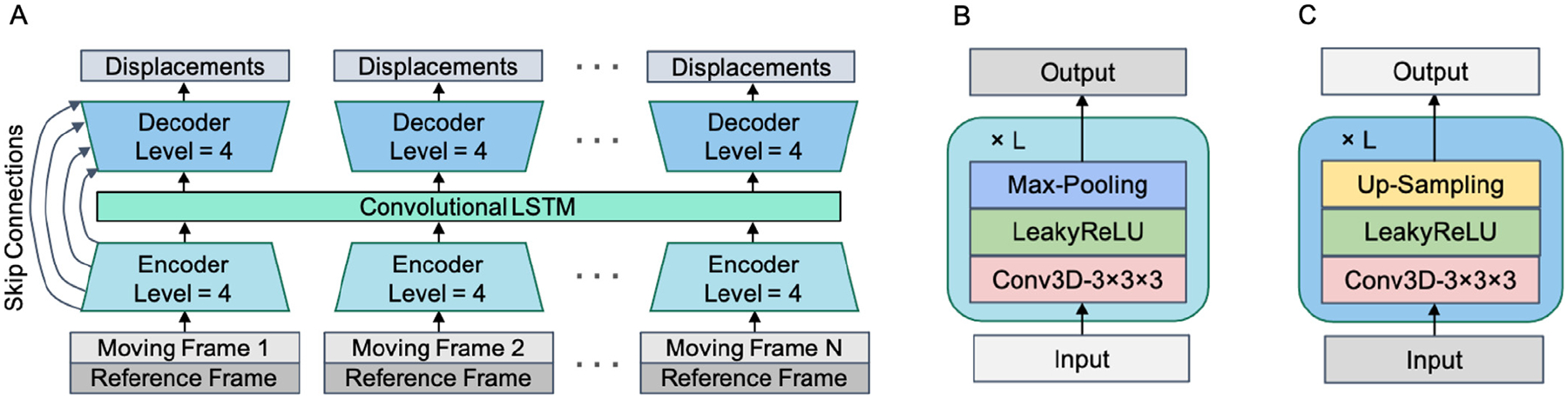
The proposed displacement estimation network B-convLSTM. (A) The network structure, a multiple-frame 3-D U-Net with a convolutional LSTM layer integrated at the bottleneck; (B) The structure of a single encoder level; (C) The structure of a single decoder level.
2.3. Model training and comparison
The inter-frame motion correction was applied to all the 5-min frames (Frame 5 - Frame 19) with Frame 12 as the reference frame. Five consecutive frames from the same subject are sent into the network at one time as the data augmentation in the temporal dimension. The input frames were downsampled by a factor of 4 and zero-padded to the same resolution of 128 × 128 × 256 due to limited GPU RAM. All dynamic frames were converted to standardized uptake values (SUV) units prior to the network input. We implemented an intensity cutoff at SUV = 2.5 with Gaussian noise (σ = 0.01) added to the thresholded voxels only for displacement computation but not the final images. The intensity cutoff is intended to mitigate the driving force from the high-intensity bladder voxels (Guo et al., 2021), and the added Gaussian noise helps avoid local saturation in the local NCC computation. The output displacement fields were then upsampled to the original resolution by a spline interpolation (order = 3) before warping the original frames.
We compared our proposed model to both traditional and deep learning motion correction baselines under the same intensity cutoff implementation. The traditional entropy-based non-rigid registration is implemented in BIS (Joshi et al., 2011), with both original and downsampled resolution images. The entropy-based normalized mutual information (NMI) was chosen as the similarity measure of BIS to support the changing tracer distribution in dynamic PET with robustness in CPU-based calculations (Wu et al., 2009). The optimization was conducted for two resolution levels with the final resolution at one half of the original resolution and step size as 2.0. The control point spacing of the free-form deformations was 50.0 mm with a spacing rate of 1.1 for lower resolution levels. All the other registration parameters in BIS were set as the default. The Voxelmorph framework (Balakrishnan et al., 2019) is selected as the deep learning image registration baseline. We implemented both single pairwise registration as in the original Voxelmorph framework and a variant using multiple-frame input to compare the performance difference between sequential input considering only more registration pairs and the temporal LSTM layer. For the multiple-frame input version with sequence length = N, the displacement estimation network is the concatenated 3-D U-Net with shared weights and batch size = N. In addition to the proposed convolutional LSTM combined at the U-Net bottleneck (B-convLSTM), we further tested two other variants: using a fully connected LSTM layer at the bottleneck (B-LSTM) to test the difference between dense and convolutional LSTM cells, and the serial implementation of the convolutional LSTM following the U-Net output (S-convLSTM) as comparison to the most common approach to combine CNNs with convolution LSTMs.
All the deep learning frameworks were implemented using Keras and TensorFlow backend and trained on a NVIDIA Quadro RTX 8000 GPU. The same downsampling strategy was applied to all the deep learning based models. The stopping epoch was chosen based on the observations of reaching the minimum validation loss, which was 750 for single pairwise Voxelmorph while that of all the multiple frame models was 500. All the networks were trained using the Adam optimizer (learning rate = 10−4 ) with batch size = 1, the same loss function, and the regularization factor λ = 1.
2.4. Motion simulation study
In real-patient datasets, the ground truth of the internal motion vectors of each voxel are typically not available. Thus, we performed a motion simulation study by applying human subjects-derived motion fields to the motion compensated frames of another subject identified as “motion-free” to directly assess motion estimation accuracy with simulated ground truth. Specifically, we selected 11 subjects with relatively insignificant motion and treated the frames after motion correction by the deep learning baseline Voxelmorph as having no motion. An affine registration was applied first to match the motion fields with the corresponding body regions of another subject and avoid large motion-related vectors appearing in the background. The Voxelmorph motion field estimations of the remaining 16 subjects with relatively significant motion were applied as the ground truth to achieve realistic motion simulations. A subject’s motion field was applied to a no-motion subject only if they were both in the test set of a cross-validation fold, resulting in 18 total simulated cases. For each motion correction approach, we computed the mean absolute prediction error in each frame and calculated the average for each subject as in Eq. (8),
| (8) |
where V is the total number of voxels per frame, () is the ground truth motion field, and () is the predicted motion field. The voxel-wise motion prediction error maps were also visualized to qualitatively compare the estimation errors.
2.5. Parametric imaging and evaluation metrics
The Patlak plot was used to analyze tracer pharmacokinetics (Patlak et al., 1983). As shown in Eq. (9), the Patlak plot was fitted voxel-wise with the dynamic frames and the input function after a starting time t* = 20 min (Ye et al., 2018; Toczek et al., 2020),
| (9) |
where is the tissue tracer concentration, is the plasma tracer concentration (input function), the slope is the net uptake rate constant, and is the y-axis intercept. This approach more easily introduces image-based regression weights to the estimation process (Carson, 2005).
The and images were overlaid to qualitatively visualize any motion-related mismatch. and are sensitive to body motion (Lu et al., 2019), where is more heavily affected by later frames while is more impacted by earlier frames. Thus, better alignment of and images signifies improved registration across the dynamic frames. The whole-body NMI as well as the whole-body NCC between and images were computed as the quantitative measurement for the alignment.
As shown in Eq. (10), the normalized weighted mean fitting errors (NFE) were computed to quantitatively assess the disparity between the dynamic data and the fitted results,
| (10) |
where is the time activity curve fitting weight after decay correction (Chen et al., 1991; 1995), is the estimated tissue tracer concentration, is the observed tissue tracer concentration, represents the middle time of the frame, and n is the number of dynamic frames after t*. The voxel-wise NFE maps were visualized as qualitative evaluation, and the NFE statistics in the whole-body, head, and ROIs were collected for quantitative evaluation.
A 9-fold subject-wise cross-validation was implemented to comprehensively evaluate the performance of all the motion correction methods. For each fold, 24 subjects were for training and the remaining 3 subjects were for testing. Significant differences between quantitative measurements from different motion correction methods were assessed using paired two-tailed t-tests with α = 0.05.
2.6. ROI Analysis
We computed the mean, maximum, and the standard deviation of the value for each ROI before and after each motion correction method was applied.
To assess the motion correction impact on benign/malignant classification capability, we concatenated the three reported features and trained four machine learning models for tumor classification: logistic regression (LR), linear support vector classifier (SVC), non-linear SVC with the radial basis function kernel, and random forest (RF). All the machine learning models were implemented using scikit-learn with all the default hyperparameters. As the ROI group is relatively small and imbalanced with more malignant lesions than benign ones, a 5-fold stratified cross validation was implemented with assigned sample weights inversely proportional to the benign/malignant ratio. For each machine learning model, the mean receiver operating characteristic (ROC) curve was generated from the mean of the sensitivity and specificity values for the 5 folds by varying the classification score thresholds, and the area under the curve (AUC) was then computed as the assessment of classification capability.
3. Results
3.1. Motion simulation study performance evaluation
The sample voxel-wise motion prediction error maps are visualized in Fig. 3. Voxelmorph produced a generally brighter error map than BIS with higher prediction error even with the ground truth motion fields predicted using the same model, potentially suggesting less generalization ability. All the multiple-frame model variants significantly decreased the motion prediction absolute errors compared with the single-pair baseline Voxelmorph (p < .05). Both S-convLSTM and Voxelmorph multiple-frame achieved similar prediction errors as compared with BIS but the S-convLSTM model further reduced the hotspots showing prediction error around body contour. The error of B-LSTM model further decreased. The B-convLSTM network generated the darkest error map among all the motion correction methods, especially at the head and body boundaries with obvious motion as well as in bladder with relatively high uptake and high prediction discrepancy. The B-convLSTM model also reached the lowest mean prediction error compared with other approaches, implying superior robustness and high prediction accuracy.
Fig. 3.

Sample absolute motion prediction error maps of the estimated motion fields for each motion correction method, with subject-wise whole-body mean absolute prediction errors (mean ± standard deviation) annotated below.
3.2. Qualitative Patlak evaluations
Fig. 4 shows the inter-frame motion impact and the correction effects on the overlaid Patlak and images. Without motion correction, the Patlak and overlaid images display spatial mis-alignments originating from the inter-frame motion. The non-rigid method of BIS substantially reduced the misalignment at the head, heart, and liver, but under-correction existed with some remaining mismatch. The performance of BIS further degraded when operating on downsampled dynamic frames, which were the same inputs used for the deep learning approaches. The baseline model Voxelmorph with single image pair input also showed similar trends, with improved alignment but remaining mismatch as well. The multi-frame version of Voxelmorph further enhanced the and alignment, showing that letting the network “see” more input frames simultaneously is a key improvement in the dynamic frame registration. The results of the B-LSTM model were even better aligned, indicating the power of recurrent analysis. Finally, the two convolutional LSTM models achieved the best visual spatial alignment improvement. Specifically, the B-convLSTM model corrected the non-rigid misalignment at the lower right brain edge and the liver boundary the best, while the S-convLSTM model reduced the misalignment from the rigid motion at the nose outline and the heart boundary the most. Note that the heart underwent significant motion and all the motion correction methods changed the spatial location and the shape of the heart, with the B-convLSTM model preserving the heart shape the best. This implies that motion correction using the multi-frame input and the convolutional LSTM for extracting spatial and temporal information could enhance the qualitative spatial alignment of the parametric images.
Fig. 4.

Sample overlaid Patlak (red) and (green) images showing inter-frame motion and correction impacts in brain (upper), heart (middle), and liver (bottom). The arrows are highlighting significant motion-related spatial mismatch and the improved alignment by motion compensation.
The significant motion impact on and misalignment could be detected in 23 out of 27 subjects; the most commonly detected voluntary movement of the head including rigid movement of the skull and the brain deformation could be found in all of the 27 subjects. Some motion-related artifacts include the “ridge-valley” artifact (Lu et al., 2019) and the same hypermetabolic peak appearing in adjacent locations in and images. According to the sample figures, the proposed spatial-temporal network was able to further reduce those artifacts and improve the motion compensation as well as lead to altered and values, though the ground truth of the and values are lacking in a real patient dataset.
The sample voxel-wise NFE maps are visualized in Fig. 5. The NFE map of the proposed network was overall darker than the maps without motion correction and other motion correction baselines under the same color bar scaling, indicating further reduced fitting error in the Patlak model. The total number of hotspot voxels representing higher voxel-wise fitting errors decreased in the sample NFE map after the proposed motion correction. For the most common head motion, the proposed networks further reduced the high error peaks at the head and brain edge. For the heart region with high fitting error due to the significant motion, the proposed networks additionally diminished the hotspots in the ventricles and at the edges. Our proposed model B-convLSTM reduced the peaks and the brightness of the NFE maps the most.
Fig. 5.

Sample voxel-wise Patlak NFE maps of skull and brain (upper) and heart (bottom). The arrows are highlighting regions with hotspots indicating high fitting error.
3.3. Quantitative Patlak evaluations
Table 2 summarizes the quantitative evaluations of the inter-frame motion correction methods. The proposed B-convLSTM network significantly reduced mean NFE in Patlak fitting in the whole-body and subareas with significant motion (head and ROIs) and raised the quantitative alignment measurements compared with traditional non-rigid and Voxelmorph baselines (all with p < .05 ). For the whole-body maximum NFE, the BIS methods tended to increase the peak values, with the average maximum NFE increasing by ~5 fold and the largest errors increasing by ~50 fold. In contrast, the proposed model successfully reduced both the lower and upper end of the peak error range. The B-convLSTM model achieved the lowest whole-body, head, and ROI NFE while the S-convLSTM attained the highest NMI and NCC, potentially indicating that the S-convLSTM model is more sensitive to matching image noise.
Table 2.
Quantitative assessments of the inter-frame motion correction methods (mean ± standard deviation, range)
| Whole-body mean NFE | Whole-body maximum NFE | Head NFE | ROI NFE | NMI | NCC | |
|---|---|---|---|---|---|---|
| Without correction | 0.1559 ± 0.0696 (0.0716 – 0.4093) |
16.1518 ± 3.6710 (7.2930 – 22.2021) |
0.1103 ± 0.0530 (0.0495 – 0.2630) |
1.3526 ± 2.1897 (0.1831 – 15.9933) |
0.9298 ± 0.0312 (0.8567 – 0.9738) |
0.2695 ± 0.1110 (0.0503 – 0.4512) |
| BIS | 0.1418 ± 0.0584 (0.0686 – 0.3671) |
70.1237 ± 245.5716 (7.2911 – 1314.6486) |
0.0915 ± 0.0442 (0.0438 – 0.2479) |
1.0298 ± 1.1165 (0.1571 – 7.4314) |
0.9451 ± 0.0283 (0.8567 – 0.9794) |
0.3150 ± 0.1067 (0.1179 – 0.5354) |
| BIS downsampled | 0.1517 ± 0.0597 (0.0730 – 0.3725) |
87.8017 ± 245.8142 (4.7684 – 1003.5248) |
0.0980 ± 0.0446 (0.0513 – 0.2594) |
1.1361 ± 1.6262 (0.1647 – 11.8469) |
0.9430 ± 0.0248 (0.8783 – 0.9736) |
0.3151 ± 0.1007 (0.1336 – 0.5079) |
| Voxelmorph | 0.1492 ± 0.0640 (0.0670 – 0.3865) |
15.2463 ± 4.0112 (7.2963 – 21.9768) |
0.1152 ± 0.0463 (0.0517 – 0.2480) |
1.3616 ± 2.0005 (0.2769 – 14.4634) |
0.9319 ± 0.0303 (0.8601 – 0.9748) |
0.2733 ± 0.1109 (0.0525 – 0.4496) |
| Voxelmorph multi-frame | 0.1181 ± 0.0476 (0.0548 – 0.3023) |
15.2255 ± 4.0066 (3.9533 – 21.5372) |
0.0801 ± 0.0385 (0.0372 – 0.2128) |
0.8949 ± 1.1831 (0.1494 – 8.4020) |
0.9540 ± 0.0219 (0.8990 – 0.9828) |
0.5021 ± 0.1639 (0.1557 – 0.7245) |
| S-convLSTM | 0.1180 ± 0.0474 (0.0573 – 0.2982) |
14.9111 ± 4.1132 (4.9149 – 21.5393) |
0.0798 ± 0.0384 (0.0378 – 0.2131) |
0.9289 ± 1.4284 (0.1472 – 10.5453) |
0.9547 ±0.0212 (0.9010 – 0.9832) |
0.5141 ±0.1524 (0.2156 – 0.7644) |
| B-LSTM | 0.1186 ± 0.0488 (0.0552 – 0.3039) |
15.2877 ± 3.6730 (6.5119 – 21.3882) |
0.0797 ± 0.0389 (0.0375 – 0.2159) |
1.0814 ± 2.3849 (0.1353 – 18.0843) |
0.9539 ± 0.0221 (0.8997 – 0.9829) |
0.4963 ± 0.1587 (0.1295 – 0.7371) |
| B-convLSTM |
0.1171 ±0.0476 (0.0547 – 0.2994) |
14.4556 ±4.3182 (4.4162 – 21.2903) |
0.0792 ±0.0383 (0.0375 – 0.2122) |
0.8690 ±1.0808 (0.1521 – 7.6837) |
0.9541 ± 0.0223 (0.8970 – 0.9832) |
0.5059 ± 0.1539 (0.1538 – 0.7691) |
The inference (wall) time of motion estimation and the model size of each motion correction method are summarized in Table 3. Note that all the deep learning models are trained under the downsampled resolution while the original BIS method used the full resolution images. Under the same downsampled resolution, the well-trained B-convLSTM model could perform motion estimation ~17 times faster than BIS and ~6 times faster than the single image pair Voxelmorph, since the multiple frame model is able to estimate the displacements in parallel. Although the multi-frame Voxelmorph model had the lowest inference time and number of parameters, the motion correction performance was significantly worse than that of the proposed B-convLSTM (Table 2). In contrast, while there were no further significant differences (p > .05) between the motion correction results of S-convLSTM and B-convLSTM, the time consumption of B-convLSTM was 11.9% lower than that of S-convLSTM with similar model size. Finally, the time consumption of B-convLSTM is only 61% of the B-LSTM model with considerably reduced model size, showing that in addition to better utilizing spatial-temporal information, another advantage of the bottleneck convolutional LSTM layer is significantly reducing the time and memory consumption.
Table 3.
The inference time of motion estimation and the model size comparison.
| Motion estimation inference time of one subject (second) | Trainable parameters | |
|---|---|---|
| BIS | 48,034 | - |
| BIS downsampled | 1813 | - |
| Voxelmorph | 642 | 327,331 |
| Voxelmorph multi-frame | 101 | 327,331 |
| S-convLSTM | 118 | 501,571 |
| B-LSTM | 170 | 138,744,355 |
| B-convLSTM | 104 | 548,643 |
Since the BIS motion correction for each pair of frames were run in parallel, we also measured the overall compute time for a fair comparison. The total compute time includes the spatial transformation time and the upsampling time for the models under the downsampled resolution in addition to the motion estimation inference time. With the displacement field upsampling and spatial warping, the overall compute time of B-convLSTM is ~65.5 min per subject (4.65 min per frame), which is still ~12 times faster than the fully parallelized original resolution BIS running 14 jobs in parallel (~13.3 hr). Without the parallel compute resource, the original BIS would take ~1 week and the downsampled BIS would need ~7.3 hours to process one subject, showing the great advantage of the savings in compute time for B-convLSTM.
3.4. ROI Analysis and malignancy classification
The statistics of the benign and malignant ROIs was listed in Table 4. All the motion correction methods suggested the general trend of reducing the mean and maximum values while increasing the standard deviation of in each ROI. The deep learning motion correction results further enhanced this impact compared with BIS, and the two convolutional LSTM networks showed similar amount of substantial change.
Table 4.
statistics of the benign and malignant ROI groups for each inter-frame motion correction method (mean ± standard deviation, range).
| Benign (n = 8) | Malignant (n = 49) | |||||
|---|---|---|---|---|---|---|
| Mean | Maximum | Standard deviation | Mean | Maximum | Standard deviation | |
| Without correction | 0.0050 ± 0.0028 (0.0017 – 0.0107) |
0.0083 ± 0.0044 (0.0024 – 0.0173) |
0.0015 ± 0.0007 (0.0003 – 0.0027) |
0.0138 ± 0.0079 (0.0009 – 0.0392) |
0.0288 ± 0.0192 (0.0017 – 0.0835) |
0.0051 ± 0.0036 (0.0002 – 0.0142) |
| BIS | 0.0049 ± 0.0028 (0.0016 – 0.0108) |
0.0083 ± 0.0046 (0.0022 – 0.0181) |
0.0014 ± 0.0007 (0.0003 – 0.0025) |
0.0134 ± 0.0077 (0.0010 – 0.0383) |
0.0287 ± 0.0187 (0.0018 – 0.0770) |
0.0053 ± 0.0037 (0.0002 – 0.0141) |
| BIS downsampled | 0.0049 ± 0.0028 (0.0016 – 0.0110) |
0.0082 ± 0.0045 (0.0023 – 0.0179) |
0.0015 ± 0.0007 (0.0003 – 0.0026) |
0.0132 ± 0.0078 (0.0008 – 0.0368) |
0.0283 ± 0.0186 (0.0019 – 0.0758) |
0.0052 ± 0.0037 (0.0002 – 0.0140) |
| Voxelmorph | 0.0043 ± 0.0031 (0.0011 – 0.0116) |
0.0076 ± 0.0045 (0.0019 – 0.0173) |
0.0015 ± 0.0007 (0.0003 – 0.0025) |
0.0119 ± 0.0074 (0.0010 – 0.0382) |
0.0271 ± 0.0183 (0.0015 – 0.0827) |
0.0053 ± 0.0039 (0.0003 – 0.0159) |
| Voxelmorph multi-frame | 0.0047 ± 0.0024 (0.0013 – 0.0094) |
0.0082 ± 0.0045 (0.0018 – 0.0168) |
0.0017 ± 0.0009 (0.0003 – 0.0031) |
0.0116 ± 0.0071 (0.0003 – 0.0344) |
0.0276 ± 0.0186 (0.0012 – 0.0743) |
0.0055 ± 0.0039 (0.0001 – 0.0150) |
| S-convLSTM | 0.0041 ± 0.0027 (0.0008 – 0.0101) |
0.0076 ± 0.0044 (0.0015 – 0.0171) |
0.0014 ± 0.0007 (0.0003 – 0.0028) |
0.0118 ± 0.0070 (0.0008 – 0.0338) |
0.0276 ± 0.0186 (0.0013 – 0.0734) |
0.0055 ± 0.0039 (0.0002 – 0.0154) |
| B-LSTM | 0.0039 ± 0.0021 (0.0014 – 0.0087) |
0.0075 ± 0.0045 (0.0021 – 0.0172) |
0.0017 ± 0.0010 (0.0003 – 0.0033) |
0.0115 ± 0.0067 (0.0007 – 0.0333) |
0.0275 ± 0.0187 (0.0012 – 0.0725) |
0.0056 ± 0.0041 (0.0002 – 0.0158) |
| B-convLSTM | 0.0041 ± 0.0024 (0.0009 – 0.0091) |
0.0075 ± 0.0045 (0.0013 – 0.0172) |
0.0015 ± 0.0010 (0.0002 – 0.0033) |
0.0118 ± 0.0068 (0.0003 – 0.0335) |
0.0277 ± 0.0183 (0.0009 – 0.0742) |
0.0054 ± 0.0039 (0.0002 – 0.0156) |
The AUCs of all the machine learning classifiers trained for hypermetabolic ROI malignancy classification from local statistics was summarized in Table 5. The average of the four (two linear and two non-linear) machine learning algorithms was also computed to assess the overall ability of distinguishing benign/malignant ROIs based on the statistics. The B-convLSTM model reached the highest average AUC with lowest standard deviation and performed best for two of the four learning methods, indicating the improved classification capability compared to other motion correction methods. Note that the ROI group is relatively small and imbalanced since all the hotspots were chosen in the cancer subjects by the physician and some of those were later categorized as benign. The average ROC curve of each inter-frame motion correction method was plotted in Supplementary Figure S1, where the curve of the B-convLSTM model exceeded that of all the other motion correction methods.
Table 5.
The AUCs of all the machine learning ROI malignancy classifiers for each motion correction method (mean ± standard deviation).
| SVC | SVC Linear | RF | LR | Average | |
|---|---|---|---|---|---|
| Without correction | 0.8500 ± 0.1483 | 0.8500 ± 0.1483 | 0.6856 ± 0.2855 | 0.8500 ± 0.1483 | 0.8008 ± 0.2151 |
| BIS | 0.8900 ± 0.1114 | 0.8700 ± 0.1166 | 0.6906 ± 0.2669 | 0.8700 ± 0.1166 | 0.8264 ± 0.2018 |
| BIS downsampled | 0.8600 ± 0.1200 | 0.8900 ± 0.1114 | 0.7578 ± 0.2486 | 0.8900 ± 0.1114 | 0.8519 ± 0.1599 |
| Voxelmorph | 0.8100 ± 0.1855 | 0.8300 ± 0.1833 | 0.7317 ± 0.2172 | 0.8300 ± 0.1833 | 0.8004 ± 0.1971 |
| Voxelmorph multi-frame | 0.8700 ± 0.1470 | 0.8500 ± 0.1483 | 0.8428 ± 0.1427 | 0.8500 ± 0.1483 | 0.8532 ± 0.1470 |
| S-convLSTM | 0.8478 ± 0.1086 | 0.8878 ± 0.0661 | 0.8528 ± 0.1045 | 0.8878 ± 0.0661 | 0.8640 ± 0.0982 |
| B-LSTM | 0.8589 ± 0.1059 | 0.8589 ± 0.1059 | 0.9228 ± 0.0404 | 0.8589 ± 0.1059 | 0.8719 ± 0.0998 |
| B-convLSTM | 0.8789 ± 0.1022 | 0.9100 ± 0.0800 | 0.9100 ± 0.1114 | 0.9100 ± 0.0800 | 0.9022 ± 0.0954 |
The sample hypermetabolic ROI images are displayed in Fig. 6. The proposed inter-frame motion correction provided additional location, edge and texture changes compared to other baselines. For the lesion of esophageal adenocarcinoma (Fig. 6 upper), the small artifact-like hotspot above the major lesion had a lower peak after the BIS correction, and the proposed B-convLSTM model further reduced its shape and values, in addition to sharpening and enhancing the edge of the lesion. For the metastatic melanoma lesion (Fig. 6 lower), the traditional baseline BIS reduced the peaks of the hot spots and amplified the tumor texture. However, the Voxelmorph deep learning baseline increased the brightness of the originally strongest hot spot. After the motion correction of the B-convLSTM model, the estimations of peak values further decreased compared to BIS. The visual differences after the proposed motion correction network might contribute to the improvement of clinical diagnosis and malignancy discrimination, although it is noted that gold standard motion-free images are not available for the real patient dataset.
Fig. 6.

Sample hypermetabolic ROI images after each inter-frame motion correction method. The arrows are highlighting significant textures.
3.5. Hyperparameter sensitivity test and ablation study
A sensitivity test was run to test the impact of regularization term lambda on the displacement field local discontinuity. According to Table 6, λ = 1 gives the lowest NFE while λ = 0.1 reaches the highest NMI and NCC. As shown in Fig. 7, λ = 1 performed the best on and spatial overlay with the least mismatch. It’s likely that the weakest penalization λ = 0.1 also matched the image noise, which caused higher intensity-based alignment but also higher NFE and more visual mismatch. With a stronger regularization (λ > 1), the model is also less effective in motion estimation. The optimal λ was set to 1, consistent with the suggestions from the original Voxelmorph study (Balakrishnan et al., 2019).
Table 6.
Quantitative assessments of the sensitivity test for regularization hyperparameter λ (mean ± standard deviation, range).
| Whole-body mean NFE | Whole-body maximum NFE | Head NFE | ROI NFE | NMI | NCC | |
|---|---|---|---|---|---|---|
| λ = 0.1 | 0.1183 ± 0.0480 (0.0567 – 0.3067) |
15.4661 ± 4.0306 (4.5706 – 21.3611) |
0.0832 ± 0.0387 (0.0394 – 0.2187) |
1.0495 ± 2.0207 (0.1789 – 15.2915) |
0.9561 ± 0.0211 (0.9017 – 0.9839) |
0.5198 ± 0.1626 (0.1866 – 0.8033) |
| λ = 1 |
0.1171 ± 0.0476 (0.0547 – 0.2994) |
14.4556 ± 4.3182 (4.4162 – 21.2903) |
0.0792 ± 0.0383 (0.0375 – 0.2122) |
0.8690 ± 1.0808 (0.1521 – 7.6837) |
0.9541 ± 0.0223 (0.8970 – 0.9832) |
0.5059 ± 0.1539 (0.1538 – 0.7691) |
| λ = 10 | 0.1239 ± 0.0523 (0.0576 – 0.3188) |
14.5822 ± 4.4000 (4.2601 – 21.6528) |
0.0821 ± 0.0391 (0.0380 – 0.2160) |
1.0364 ± 1.8285 (0.1373 – 13.8209) |
0.9492 ± 0.0237 (0.8930 – 0.9820) |
0.4384 ± 0.1408 (0.1547 – 0.7410) |
| λ = 100 | 0.1342 ± 0.0576 (0.0644 – 0.3466) |
15.0293 ± 4.4169 (6.9871 – 21.9813) |
0.0906 ± 0.0434 (0.0410 – 0.2311) |
1.0449 ± 1.2975 (0.1917 – 9.1753) |
0.9395 ± 0.0275 (0.8724 – 0.9784) |
0.3182 ± 0.1101 (0.1094 – 0.5402) |
Fig. 7.

The sample overlaid (red) / (green) images of the sensitivity test, with the arrows highlighting significant spatial mismatch and motion correction effect. (A) λ = 0.1; (B) λ = 1; (C) λ = 10; (D) λ = 100.
In addition to the regularization factor λ, there are several other model settings worth investigation such as the image similarity metric, upsampling and downsampling strategies, and the input temporal resolution represented by the sequence length N. Note that this paper mainly focuses on the investigation of the multiple-frame input and the spatial-temporal structure of inter-frame motion correction network, and all the deep learning variants follow the same model settings. Thus, an additional ablation study briefly evaluating other factors is implemented on a sample fold of the cross-validation. As shown in Supplementary Figure S2, the B-convLSTM model with NCC as image similarity loss term, max-pooling/upsampling as the downsampling/upsampling strategy, and the input length = 5 gained the best spatial alignment. The artifacts of expansion in liver dome region are observed with NMI as the image similarity loss. The model with the striding/transpose convolution strategy had larger residual mismatch in kidney and GI tract. In addition to the proposed spatial-temporal model outperforming the single-pair network baseline, the advantage of temporal analysis is also shown in the degraded visual performance in B-convLSTM with input length = 3. The similar trend is also shown in Supplementary Table S1 where the proposed B-convLSTM achieved the lowest NFE.
4. Discussion
In this work, we proposed the usage of convolutional LSTM integrated into a deep convolutional network for fast inter-frame motion correction in dynamic PET and parametric imaging. The network allows the model to “see” multiple dynamic image series as the input together and process the spatial-temporal information and features. Compared to traditional and deep learning baselines, the proposed method successfully further reduced motion prediction error and enhanced the spatial alignment of the parametric and images and reduced inter-frame mismatch. The Patlak NFE was significantly reduced in the whole-body, head and ROI subareas, which exhibited considerable motion. The further modifications of the ROI appearances were observed with greater texture and shape change, and the potential of further improving the benign/malignant classification capacity following motion correction with our B-convLSTM model was suggested. Once trained, it takes ~4.65 min/frame to apply the proposed motion correction model, substantially reducing the time consumption compared with the traditional BIS method (~13.3 hr/frame).
A major obstacle holding back the clinical application of BIS motion correction is the needed long computing time. Using downsampled dynamic frames as the input was able to speed up the process (~31 min/frame), but the registration performance also degraded due to the lower resolution. Due to the memory limitation, the proposed motion correction network was inputted with the downsampled dynamic frame series, and the results computed based on a lower resolution still achieved greater qualitative and quantitative performances than the full-resolution BIS. The length of the input frame sequences for the proposed model was fixed at 5, which was limited by the GPU memory resource, although the high memory and computational resource requirement are from the 4-D whole-body data. Therefore, the network has the potential to be extended for longer time sequences with lower resolution such as cardiac motion tracking and prediction.
Compared to the deep learning baseline Voxelmorph with one single image pair, the Voxelmorph multi-frame showed that it is promising to have sequential inputs and the multiple frame pair registration for the dynamic PET images with related inter-frame kinetic information. We then demonstrated the advantage of integrating an LSTM layer into the multiple frame network by experimenting with three models: S-convLSTM, with a convolutional LSTM layer serially following the multi-frame Voxelmorph network; B-LSTM, with a standard fully-connected LSTM layer implemented at the bottleneck of the U-Net in the multiframe Voxelmorph network; and our proposed B-convLSTM, with a convolutional LSTM layer integrated into the bottleneck of the U-Net. The input feature map size for models with sequential connections is considerably larger than the bottleneck integration, making an S-LSTM (serial fully connected LSTM following the U-Net output) intractable, and thus only B-LSTM was tested. Compared with the fully connected LSTM, the convolutional LSTM showed its superiority in extracting spatial and temporal information simultaneously from the 4-D image series while also saving the computation and memory resources. The two ways of integrating the convolutional LSTM layer, i.e., S-convLSTM and B-convLSTM, both showed advantages in some aspects. While S-convLSTM reached the closest alignment, the B-convLSTM model achieved the lowest Patlak fitting error with less soft tissue shape distortion and produced estimates that resulted in the greatest ability to distinguish tumor malignancy. Moreover, with the smaller input and output feature map size, the B-convLSTM model is more practical in actual implementation with less GPU memory exhaustion.
Since the motion-free gold standard dynamic images as well as the Patlak and images are not available for the real dataset, the motion impact on Patlak quantification was evaluated by a tumor phantom motion simulation. Pseudo local shift and expansion/contraction were applied to the dynamic frames of a tumor phantom, and the images as well as the and Patlak error statistics were evaluated. As shown in Supplementary Figure S3 and Table S2, motion introduces artifacts and overestimation of . Thus, motion correction is expected to generate lower values in the lesion, which is consistent with our human study results presented in this paper. Additionally, a sample Patlak plot of one hypermetabolic ROI before and after motion correction is shown in Supplementary Figure S4, further demonstrating the change in values.
The impact of motion has been investigated in static PET (Liu et al., 2009) and single-bed dynamic PET (Lu et al., 2019) in prior studies. In the whole-body scope, we evaluated the real patient motion impact on Patlak and image spatial alignment by a motion simulation test similar to the motion prediction test. Specifically, the dynamic frames after motion correction by B-convLSTM with minimal residual motion were selected as the no-motion gold standard. Then, displacement fields from other subjects classified as minor motion and significant motion were applied to the dynamic frames. A significant motion field scaled by a factor = 2 was applied as the most severe motion. In Supplementary Figure S5, from no motion (minimal residual motion) to the most severe motion, the spatial misalignment between and images becomes stronger, showing the impact of motion in Patlak analysis.
The sensitivity of motion correction to different levels of motion was studied by plotting a scatter plot of percentage motion prediction error vs. the motion magnitude ground truth of each voxel. In Supplementary Figure S6, as the voxel displacement magnitude increases, the percentage prediction error of both BIS and B-convLSTM generally decreases. Most of the motion vectors with extremely high percentage prediction error have magnitude far less than the image voxel size (2 mm) and scanner resolution (4 mm), which is consistent with prior respiratory motion studies (Chan et al., 2017). The B-convLSTM improved the motion prediction accuracy with lower percentage prediction error compared with BIS. Although the prior study used external motion tracking-derived vectors for ground truth motion while our study used the non-rigid whole-body motion estimated from another subject as ground truth, our inter-frame motion correction study still shows low prediction error even with the potential inaccurate motion ground truth and minimal residual motion. In Supplementary Figure S7, the overlaid dynamic frames showed that the B-convLSTM model will not introduce new motion when being applied on a motion-free case. When applied on the sample case with motion, the B-convLSTM model predicted motion fields with a mean magnitude of 0.784 mm and maximum magnitude of 4.000 mm. On the motion-free (i.e., motion-corrected) case, the mean motion magnitude decreased to 0.099 mm and the maximum magnitude to 1.101 mm.
There are several limitations in this work, leading to further investigations. First, our current work focuses on the inter-frame motion that causes inter-frame mismatch, including the long-term respiratory and cardiac motion pattern change and the voluntary body movement. However, the intra-frame respiratory, cardiac, and body motion could also degrade the reconstructed image quality and lead to blur, introducing quantification error in parametric imaging as well. A potential future direction is combining the inter-frame and intra-frame motion correction, which is expected to further reduce the parametric fitting error. Given that the time and computation consumption of current intra-frame motion correction methods is very high (Mohy-ud-Din et al., 2015), it will be worth investigating a deep learning approach and building a joint intra-inter-frame motion correction network. Second, the current proposed network only considers the inter-frame motion correction problem, and the target parametric estimation is then separately implemented by Patlak fitting. To fully take advantage of the tracer kinetics and the inter-frame temporal dependence, future work could include joint parametric imaging with the inter-frame motion correction to directly optimize the Patlak fitting error. Such an end-to-end framework would be more efficient and convenient for potential clinical applications.
In addition to the current limitations, some potential future directions are worth investigating. With other datasets under different tracers and imaging protocols, we could test the robustness of the proposed motion correction model. Transfer learning could also be applied for the model to generalize across different tracers, scanners, and imaging protocols. Also, the attention mechanism (Vaswani et al., 2017) has been proposed in natural language processing and shown its superiority in video capturing (Cai and Wei, 2020) and CT image segmentation (Oktay et al., 2018). Introducing the attention mechanism into our motion correction model may help further correct the subareas with significant motion and improve the model performance. Finally, the backbone of the network is interchangeable and not limited to the U-Net used in this work. For example, Transformer based models have been widely used in a variety of natural language tasks (Gillioz et al., 2020), and has been recently reported in image generation (Parmar et al., 2018) and image restoration (Wang et al., 2021b). It is worth investigating various backbone structures and further improve the model performance and efficiency.
5. Conclusion
In this work, we presented a new deep learning inter-frame motion correction method for dynamic PET and parametric imaging. Our proposed model integrated a convolutional LSTM layer into the bottleneck of a U-net style convolutional network to estimate motion across multiple dynamic PET frames. Compared with both traditional and deep learning baseline methods, the proposed model successfully further reduced the motion prediction error in the motion simulation study as well as reduced Patlak NFE and enhanced spatial alignment of the Patlak and images in real patient data. In hypermetabolic ROIs, notable additional value changes and tumor texture changes were observed, with improved benign/malignant classification capability after correcting for motion with our proposed model. The well-trained network could perform motion estimation at around 7.4 seconds per frame, and the entire motion correction pipeline consumed only 1/12 of the wall time for the fully parallelized traditional BIS method and 1/170 of the overall compute time for BIS. Our proposed method demonstrated the potential of introducing multiple-frame analysis and extracting spatial and temporal information for correcting motion in dynamic PET images.
Supplementary Material
Acknowledgments
This work was under the support of the National Institutes of Health (NIH) through grant R01 CA224140 and a research contract from Siemens Medical Solutions USA, Inc.
Footnotes
Declaration of Competing Interest
David Pigg, Bruce Spottiswoode and Michael E. Casey are employees of Siemens Medical Solutions USA, Inc. No other potential conflicts of interest relevant to this article exist.
CRediT authorship contribution statement
Xueqi Guo: Conceptualization, Methodology, Software, Validation, Formal analysis, Investigation, Data curation, Writing – original draft, Writing – review & editing, Visualization. Bo Zhou: Methodology, Writing – review & editing. David Pigg: Writing – review & editing. Bruce Spottiswoode: Writing – review & editing. Michael E. Casey: Writing – review & editing, Funding acquisition. Chi Liu: Conceptualization, Writing – review & editing, Supervision, Funding acquisition. Nicha C. Dvornek: Conceptualization, Methodology, Writing – review & editing, Supervision.
Supplementary material
Supplementary material associated with this article can be found, in the online version, at doi: 10.1016/j.media.2022.102524.
References
- Abdi AH, Luong C, Tsang T, Jue J, Gin K, Yeung D, Hawley D, Rohling R, Abol-maesumi P, 2017. Quality assessment of echocardiographic cine using recurrent neural networks: Feasibility on five standard view planes. In: International Conference on Medical Image Computing and Computer-Assisted Intervention. Springer, pp. 302–310. [Google Scholar]
- Arbelle A, Raviv TR, 2019. Microscopy cell segmentation via convolutional lstm networks. In: 2019 IEEE 16th International Symposium on Biomedical Imaging (ISBI 2019). IEEE, pp. 1008–1012. [Google Scholar]
- Azad R, Asadi-Aghbolaghi M, Fathy M, Escalera S, 2019. Bi-directional convlstm u-net with densley connected convolutions. In: Proceedings of the IEEE/CVF International Conference on Computer Vision Workshops. 0–0 [Google Scholar]
- Azizmohammadi F, Martin R, Miro J, Duong L, 2019. Model-free cardiorespiratory motion prediction from x-ray angiography sequence with lstm network. In: 2019 41st Annual International Conference of the IEEE Engineering in Medicine and Biology Society (EMBC). IEEE, pp. 7014–7018. [DOI] [PubMed] [Google Scholar]
- Balakrishnan G, Zhao A, Sabuncu MR, Guttag J, Dalca AV, 2019. Voxelmorph: a learning framework for deformable medical image registration. IEEE Trans. Med. Imaging 38 (8), 1788–1800. [DOI] [PubMed] [Google Scholar]
- Cai W, Wei Z, 2020. Remote sensing image classification based on a cross-attention mechanism and graph convolution. IEEE Geosci. Remote Sens. Lett. [Google Scholar]
- Carson RE, 2005. Tracer Kinetic Modeling in Pet. In: Positron Emission Tomography. Springer, pp. 127–159. [Google Scholar]
- Chan C, Onofrey J, Jian Y, Germino M, Papademetris X, Carson RE, Liu C, 2017. Non-rigid event-by-event continuous respiratory motion compensated list-mode reconstruction for pet. IEEE Trans. Med. Imaging 37 (2), 504–515. [DOI] [PMC free article] [PubMed] [Google Scholar]
- Chen J, Yang L, Zhang Y, Alber M, Chen DZ, 2016. Combining fully convolutional and recurrent neural networks for 3d biomedical image segmentation. In: Advances in neural information processing systems, pp. 3036–3044. [Google Scholar]
- Chen K, Huang S-C, Yu D-C, 1991. The effects of measurement errors in the plasma radioactivity curve on parameter estimation in positron emission tomography. Physics in Medicine & Biology 36 (9), 1183. [DOI] [PubMed] [Google Scholar]
- Chen K, Reiman E, Lawson M, Feng D, Huang S-C, 1995. Decay correction methods in dynamic pet studies. IEEE Trans. Nucl. Sci 42 (6), 2173–2179. [Google Scholar]
- Cho K, Van Merriënboer B, Gulcehre C, Bahdanau D, Bougares F, Schwenk H, Bengio Y, 2014. Learning phrase representations using rnn encoder-decoder for statistical machine translation. arXiv preprint arXiv:1406.1078. [Google Scholar]
- Çiçek Ö, Abdulkadir A, Lienkamp SS, Brox T, Ronneberger O, 2016. 3d u-net: learning dense volumetric segmentation from sparse annotation. In: International conference on medical image computing and computer-assisted intervention. Springer, pp. 424–432. [Google Scholar]
- Dimitrakopoulou-Strauss A, Pan L, Sachpekidis C, 2021. Kinetic modeling and parametric imaging with dynamic pet for oncological applications: general considerations, current clinical applications, and future perspectives. Eur. J. Nucl. Med. Mol. Imaging 48, 21–39. [DOI] [PMC free article] [PubMed] [Google Scholar]
- Dvornek NC, Ventola P, Pelphrey KA, Duncan JS, 2017. Identifying autism from resting-state fmri using long short-term memory networks. In: International Workshop on Machine Learning in Medical Imaging. Springer, pp. 362–370. [DOI] [PMC free article] [PubMed] [Google Scholar]
- Fahrni G, Karakatsanis NA, Di Domenicantonio G, Garibotto V, Zaidi H, 2019. Does whole-body patlak 18 f-fdg pet imaging improve lesion detectability in clinical oncology? Eur. Radiol 29 (9), 4812–4821. [DOI] [PubMed] [Google Scholar]
- Fayad H, Odille F, Schmidt H, Würslin C, Küstner T, Felblinger J, Visvikis D, 2015. The use of a generalized reconstruction by inversion of coupled systems (grics) approach for generic respiratory motion correction in pet/mr imaging. Phys. Med. Biol 60 (6), 2529. [DOI] [PubMed] [Google Scholar]
- Feng T, Wang J, Sun Y, Zhu W, Dong Y, Li H, 2017. Self-gating: an adaptive center-of-mass approach for respiratory gating in pet. IEEE Trans. Med. Imaging 37 (5), 1140–1148. [DOI] [PubMed] [Google Scholar]
- Gallezot J-D, Lu Y, Naganawa M, Carson RE, 2019. Parametric imaging with pet and spect. IEEE Transact. Radiat. Plasma Med. Sci 4 (1), 1–23. [Google Scholar]
- Ge H, Yan Z, Yu W, Sun L, 2019. An attention mechanism based convolutional lstm network for video action recognition. Multimed. Tool. Appl 78 (14), 20533–20556. [Google Scholar]
- Gillioz A, Casas J, Mugellini E, Abou Khaled O, 2020. Overview of the transformer-based models for nlp tasks. In: 2020 15th Conference on Computer Science and Information Systems (FedCSIS). IEEE, pp. 179–183. [Google Scholar]
- Guo X, Tinaz S, Dvornek NC, 2022. Characterization of Early Stage Parkinson’s Disease from Resting-state fMRI Data Using a Long Short-term Memory Network. Frontiers in Neuroimaging doi: 10.3389/fnimg.2022.952084. [DOI] [PMC free article] [PubMed] [Google Scholar]
- Guo Y, Dvornek N, Lu Y, Tsai Y-J, Hamill J, Casey M, Liu C, 2019. Deep learning based respiratory pattern classification and applications in pet/ct motion correction. In: 2019 IEEE Nuclear Science Symposium and Medical Imaging Conference (NSS/MIC). IEEE, pp. 1–5. [Google Scholar]
- Guo X, Wu J, Chen M-K, Onofrey J, Pang Y, Pigg D, Casey M, Dvornek N, Liu C, 2021. Inter-pass motion correction for whole-body dynamic parametric pet imaging. J. Nucl. Med 62 (supplement 1), 1421. [DOI] [PMC free article] [PubMed] [Google Scholar]
- Hanson A, Pnvr K, Krishnagopal S, Davis L, 2018. Bidirectional convolutional lstm for the detection of violence in videos. In: Proceedings of the European Conference on Computer Vision (ECCV) Workshops. 0–0 [Google Scholar]
- Hochreiter S, Schmidhuber J, 1997. Long short-term memory. Neural Comput 9 (8), 1735–1780. [DOI] [PubMed] [Google Scholar]
- Huang W, Bridge CP, Noble JA, Zisserman A, 2017. Temporal heartnet: towards human-level automatic analysis of fetal cardiac screening video. In: International Conference on Medical Image Computing and Computer-Assisted Intervention. Springer, pp. 341–349. [Google Scholar]
- Hudson HM, Larkin RS, 1994. Accelerated image reconstruction using ordered subsets of projection data. IEEE Trans. Med. Imaging 13 (4), 601–609. [DOI] [PubMed] [Google Scholar]
- Joshi A, Scheinost D, Okuda H, Belhachemi D, Murphy I, Staib LH, Papademetris X, 2011. Unified framework for development, deployment and robust testing of neuroimaging algorithms. Neuroinformatics 9 (1), 69–84. [DOI] [PMC free article] [PubMed] [Google Scholar]
- Karakatsanis NA, Lodge MA, Tahari AK, Zhou Y, Wahl RL, Rahmim A, 2013. Dynamic whole-body pet parametric imaging: i. concept, acquisition protocol optimization and clinical application. Phys. Med. Biol 58 (20), 7391. [DOI] [PMC free article] [PubMed] [Google Scholar]
- Küstner T, Schwartz M, Martirosian P, Gatidis S, Seith F, Gilliam C, Blu T, Fayad H, Visvikis D, Schick F, et al. , 2017. Mr-based respiratory and cardiac motion correction for pet imaging. Med. Image Anal 42, 129–144. [DOI] [PubMed] [Google Scholar]
- Lamare F, Le Maitre A, Dawood M, Schäfers K, Fernandez P, Rimoldi O, Visvikis D, 2014. Evaluation of respiratory and cardiac motion correction schemes in dual gated pet/ct cardiac imaging. Med. Phys 41 (7), 072504. [DOI] [PubMed] [Google Scholar]
- Li M, Wang C, Zhang H, Yang G, 2020. Mv-ran: multiview recurrent aggregation network for echocardiographic sequences segmentation and full cardiac cycle analysis. Comput. Biol. Med 120, 103728. [DOI] [PubMed] [Google Scholar]
- Li M, Zhang W, Yang G, Wang C, Zhang H, Liu H, Zheng W, Li S, 2019. Recurrent aggregation learning for multi-view echocardiographic sequences segmentation. In: International Conference on Medical Image Computing and Computer-Assisted Intervention. Springer, pp. 678–686. [Google Scholar]
- Li T, Zhang M, Qi W, Asma E, Qi J, 2020. Motion correction of respiratory-gated pet images using deep learning based image registration framework. Phys. Med. Biol 65 (15), 155003. [DOI] [PMC free article] [PubMed] [Google Scholar]
- Liu C, Pierce LA II, Alessio AM, Kinahan PE, 2009. The impact of respiratory motion on tumor quantification and delineation in static pet/ct imaging. Phys. Med. Biol 54 (24), 7345. [DOI] [PMC free article] [PubMed] [Google Scholar]
- Lu Y, Fontaine K, Mulnix T, Onofrey JA, Ren S, Panin V, Jones J, Casey ME, Barnett R, Kench P, et al. , 2018. Respiratory motion compensation for pet/ct with motion information derived from matched attenuation-corrected gated pet data. J. Nucl. Med 59 (9), 1480–1486. [DOI] [PMC free article] [PubMed] [Google Scholar]
- Lu Y, Gallezot J-D, Naganawa M, Ren S, Fontaine K, Wu J, Onofrey JA, Toyonaga T, Boutagy N, Mulnix T, et al. , 2019. Data-driven voluntary body motion detection and non-rigid event-by-event correction for static and dynamic pet. Phys. Med. Biol 64 (6), 065002. [DOI] [PubMed] [Google Scholar]
- Lu Y, Naganawa M, Toyonaga T, Gallezot J-D, Fontaine K, Ren S, Revilla EM, Mulnix T, Carson RE, 2020. Data-driven motion detection and event-by-event correction for brain pet: comparison with vicra. J. Nucl. Med 61 (9), 1397–1403. [DOI] [PMC free article] [PubMed] [Google Scholar]
- Manber R, Thielemans K, Hutton BF, Wan S, McClelland J, Barnes A, Arridge S, Ourselin S, Atkinson D, 2016. Joint pet-mr respiratory motion models for clinical pet motion correction. Phys. Med. Biol 61 (17), 6515. [DOI] [PubMed] [Google Scholar]
- Medsker LR, Jain L, 2001. Recurrent neural networks. Des. Applica 5 . [Google Scholar]
- Merity S, Keskar NS, Socher R, 2017. Regularizing and optimizing lstm language models. arXiv preprint arXiv:1708.02182 . [Google Scholar]
- Mohy-ud-Din H, Nicolas A, Willis W, Abdel K, Dean F, Rahmim A, et al. , 2015. Intra-frame motion compensation in multi-frame brain pet imaging. Front. Biomed. Technol 2 (2), 60–72 . [Google Scholar]
- Muzi M, O’Sullivan F, Mankoff DA, Doot RK, Pierce LA, Kurland BF, Linden HM, Kinahan PE, 2012. Quantitative assessment of dynamic pet imaging data in cancer imaging. Magn. Reson. Imaging 30, 1203–1215 . [DOI] [PMC free article] [PubMed] [Google Scholar]
- Naganawa M, Gallezot J-D, Shah V, Mulnix T, Young C, Dias M, Chen M-K, Smith AM, Carson RE, 2020. Assessment of population-based input functions for patlak imaging of whole body dynamic 18 f-fdg pet. EJNMMI Phys 7 (1), 1–15 . [DOI] [PMC free article] [PubMed] [Google Scholar]
- Noonan P, Howard J, Hallett W, Gunn R, 2015. Repurposing the microsoft kinect for windows v2 for external head motion tracking for brain pet. Phys. Med. Biol 60 (22), 8753. [DOI] [PubMed] [Google Scholar]
- Oktay O, Schlemper J, Folgoc LL, Lee M, Heinrich M, Misawa K, Mori K, Mc-Donagh S, Hammerla NY, Kainz B, et al. , 2018. Attention u-net: learning where to look for the pancreas. arXiv preprint arXiv:1804.03999 . [Google Scholar]
- Panin VY, Smith AM, Hu J, Kehren F, Casey ME, 2014. Continuous bed motion on clinical scanner: design, data correction, and reconstruction. Phys. Med. Biol 59 (20), 6153. [DOI] [PubMed] [Google Scholar]
- Parmar N, Vaswani A, Uszkoreit J, Kaiser L, Shazeer N, Ku A, Tran D, 2018. Image transformer. In: International Conference on Machine Learning. PMLR, pp. 4055–4064 . [Google Scholar]
- Patlak CS, Blasberg RG, Fenstermacher JD, 1983. Graphical evaluation of blood-to-brain transfer constants from multiple-time uptake data. J. Cereb. Blood Flow Metab 3 (1), 1–7 . [DOI] [PubMed] [Google Scholar]
- Ronneberger O, Fischer P, Brox T, 2015. U-net: Convolutional networks for biomedical image segmentation. In: International Conference on Medical image computing and computer-assisted intervention. Springer, pp. 234–241 . [Google Scholar]
- Sandkühler R, Andermatt S, Bauman G, Nyilas S, Jud C, Cattin PC, 2019. Recurrent registration neural networks for deformable image registration. Adv. Neural Inf. Process. Syst 32, 8758–8768 . [Google Scholar]
- Shi L, Lu Y, Dvornek N, Weyman CA, Miller EJ, Sinusas AJ, Liu C, 2021. Automatic inter-frame patient motion correction for dynamic cardiac pet using deep learning. IEEE Trans. Med. Imaging . [DOI] [PMC free article] [PubMed] [Google Scholar]
- Shi X, Chen Z, Wang H, Yeung D-Y, Wong W-K, Woo W. c., 2015. Convolutional lstm network: a machine learning approach for precipitation nowcasting. arXiv preprint arXiv:1506.04214 . [Google Scholar]
- Sundar LKS, Iommi D, Muzik O, Chalampalakis Z, Klebermass E-M, Hienert M, Rischka L, Lanzenberger R, Hahn A, Pataraia E, et al. , 2021. Conditional generative adversarial networks aided motion correction of dynamic 18f-fdg pet brain studies. J. Nucl. Med 62 (6), 871–880. [DOI] [PMC free article] [PubMed] [Google Scholar]
- Toczek J, Wu J, Hillmer AT, Han J, Esterlis I, Cosgrove KP, Liu C, Sadeghi MM, 2020. Accuracy of arterial [18 f]-fluorodeoxyglucose uptake quantification: a kinetic modeling study. J. Nuclear Cardiol 1–4 . [DOI] [PMC free article] [PubMed] [Google Scholar]
- Tsoumpas C, Buerger C, King A, Mollet P, Keereman V, Vandenberghe S, Schulz V, Schleyer P, Schaeffter T, Marsden P, 2011. Fast generation of 4d pet-mr data from real dynamic mr acquisitions. Phys. Med. Biol 56 (20), 6597. [DOI] [PubMed] [Google Scholar]
- Vaswani A, Shazeer N, Parmar N, Uszkoreit J, Jones L, Gomez AN, Kaiser Ł, Polosukhin I, 2017. Attention is all you need. In: Advances in neural information processing systems, pp. 5998–6008 . [Google Scholar]
- Wang G, Li Z, Li G, Dai G, Xiao Q, Bai L, He Y, Liu Y, Bai S, 2021. Real–time liver tracking algorithm based on lstm and svr networks for use in surface-guided radiation therapy. Radiat. Oncol 16 (1), 1–12 . [DOI] [PMC free article] [PubMed] [Google Scholar]
- Wang Z, Cun X, Bao J, Liu J, 2021. Uformer: a general u-shaped transformer for image restoration. arXiv preprint arXiv:2106.03106 . [Google Scholar]
- Wright R, Khanal B, Gomez A, Skelton E, Matthew J, Hajnal JV, Rueckert D, Schnabel JA, 2018. Lstm spatial co-transformer networks for registration of 3d fetal us and mr brain images. In: Data Driven Treatment Response Assessment and Preterm, Perinatal, and Paediatric Image Analysis. Springer, pp. 149–159 . [Google Scholar]
- Wu J, Kim M, Peters J, Chung H, Samant SS, 2009. Evaluation of similarity measures for use in the intensity-based rigid 2d-3d registration for patient positioning in radiotherapy. Med. Phys 36 (12), 5391–5403 . [DOI] [PubMed] [Google Scholar]
- Xue W, Brahm G, Pandey S, Leung S, Li S, 2018. Full left ventricle quantification via deep multitask relationships learning. Med. Image Anal 43, 54–65 . [DOI] [PubMed] [Google Scholar]
- Yang X, Kwitt R, Styner M, Niethammer M, 2017. Quicksilver: fast predictive image registration–a deep learning approach. Neuroimage 158, 378–396 . [DOI] [PMC free article] [PubMed] [Google Scholar]
- Ye Q, Wu J, Lu Y, Naganawa M, Gallezot J-D, Ma T, Liu Y, Tanoue L, Detterbeck F, Blasberg J, et al. , 2018. Improved discrimination between benign and malignant ldct screening-detected lung nodules with dynamic over static 18f-fdg pet as a function of injected dose. Phys. Med. Biol 63 (17), 175015. [DOI] [PMC free article] [PubMed] [Google Scholar]
- Zeng Q, Fu Y, Jeong J, Lei Y, Wang T, Mao H, Jani AB, Patel P, Curran WJ, Liu T, et al. , 2020. Weakly non-rigid mr-trus prostate registration using fully convolutional and recurrent neural networks. In: Medical Imaging 2020: Image Processing, Vol. 11313. International Society for Optics and Photonics, p. 113132Y. [Google Scholar]
- Zhang D, Icke I, Dogdas B, Parimal S, Sampath S, Forbes J, Bagchi A, Chin C-L, Chen A, 2018. A multi-level convolutional lstm model for the segmentation of left ventricle myocardium in infarcted porcine cine mr images. In: 2018 IEEE 15th International Symposium on Biomedical Imaging (ISBI 2018). IEEE, pp. 470–473 . [Google Scholar]
- Zhang D, Icke I, Dogdas B, Parimal S, Sampath S, Forbes J, Bagchi A, Chin C-L, Chen A, 2018. Segmentation of left ventricle myocardium in porcine cardiac cine mr images using a hybrid of fully convolutional neural networks and convolutional lstm. In: Medical Imaging 2018: Image Processing, Vol. 10574. International Society for Optics and Photonics, p. 105740A. [Google Scholar]
- Zhao S, Lau T, Luo J, Eric I, Chang C, Xu Y, 2019. Unsupervised 3d end-to-end medical image registration with volume tweening network. IEEE J. Biomed. Health Inform 24 (5), 1394–1404 . [DOI] [PubMed] [Google Scholar]
- Zhou B, Tsai Y-J, Chen X, Duncan JS, Liu C, 2021. Mdpet: a unified motion correction and denoising adversarial network for low-dose gated pet. IEEE Trans. Med. Imaging . [DOI] [PMC free article] [PubMed] [Google Scholar]
- Ziegler SI, 2005. Positron emission tomography: principles, technology, and recent developments. Nucl. Phys. A 752, 679–687 . [Google Scholar]
Associated Data
This section collects any data citations, data availability statements, or supplementary materials included in this article.