Heritability estimation approaches utilizing genome-wide data

Abstract

Prior to the development of genome-wide arrays and whole genome sequencing technologies, heritability estimation mainly relied on the study of related individuals. Over the past decade, various approaches have been developed to estimate SNP-based narrow-sense heritability (${\mathrm{h}}_{\mathrm{S}\mathrm{N}\mathrm{P}}^2$) in unrelated individuals. These latter approaches use either individual-level genetic variations or summary results from genome-wide association studies (GWAS). Recently, several studies compared these approaches using extensive simulations and empirical datasets. However, sparse information on hands-on training necessitates revisiting these approaches from the perspective of a stepwise guide for practical applications. Here, we provide an overview of the commonly used SNP-heritability estimation approaches utilizing genome-wide array, imputed or whole genome data from unrelated individuals or summary results. We not only discuss these approaches based on their statistical concepts, utility, advantages and limitations but also provide step-by-step protocols to apply these approaches. For illustration purposes, we estimate ${\mathrm{h}}_{\mathrm{S}\mathrm{N}\mathrm{P}}^2$ of height and BMI utilizing individual-level data from The Northern Finland Birth Cohort (NFBC; available through dbGaP; see link) and summary results from the Genetic Investigation of ANthropometric Traits (GIANT; see link) consortium. We present this review as a template for the researchers who estimate and use heritability in their studies and as a reference for geneticists who develop or extend heritability estimation approaches.

Introduction

A long-standing question in quantitative and behavioral genetics is whether the variation in a particular trait is due to genetic or environmental factors (Visscher, Hill, & Wray, 2008). A key step in finding an answer to this question is partitioning the observed phenotypic variance into variance components attributable to unobserved genetic and environmental factors. R. A. Fisher (Fisher, 1918) first modeled and partitioned the phenotypic variance into genetic and environmental components without any knowledge of specific genes affecting the trait (Visscher & Goddard, 2019). Although he didn’t use the term ‘heritability’, his research laid the foundation for various future approaches for the estimation of heritability (Falconer, 1960; Walsh, 1998).

Heritability is defined as the proportion of phenotypic variance that is attributable to genetic factors in a given population at a specific time(Falconer, 1960; Walsh, 1998). Heritability can be defined in two ways. The broad-sense heritability (H²) estimates the proportion of phenotypic variance attributable to all genetic factors, including additive genetic effects (A), dominant genetic effects (D), and epistatic effects (G x G)(Mayhew & Meyre, 2017; Visscher et al., 2008; Zhu & Zhou, 2020). In contrast, narrow-sense heritability (h²) estimates the proportion of phenotypic variance attributable to additive genetic effects (A) or breeding values(Mayhew & Meyre, 2017; Visscher et al., 2008; Zhu & Zhou, 2020). Since h² is more relevant to the evaluation of genetic influence on phenotypic resemblance of relatives and predicting evolutionary responses to selection, it is a commonly used parameter for heritability estimation and applications(Visscher et al., 2008).

Heritability plays an important role in several areas of biology such as agriculture, medicine and evolution(Visscher et al., 2008). It facilitates selective breeding programs to improve the quality of plant and domestic animals(Alvarez, 2017; Bernardo, 2020; Berry et al., 2003; Berry, Wall, & Pryce, 2014; Cassell, 2009; Manjula et al., 2018; Miglior et al., 2017; Palmquist & Jenkins, 2017; Utrera & Van Vleck, 2004; Velasco & Fernández-martínez, 2002). Heritability also provides insights into the genetic architecture of complex traits and related diseases (Eichler et al., 2010; Friedman, Banich, & Keller, 2021; Lunde, Melve, Gjessing, Skjaerven, & Irgens, 2007; Manolio et al., 2009; Silventoinen et al., 2003; Tenesa & Haley, 2013; Vinkhuyzen, Wray, Yang, Goddard, & Visscher, 2013; Visscher et al., 2007; Wray, Goddard, & Visscher, 2007). For over a century, heritability has played a key role in measuring the genetic influence on various traits and diseases (Dempster & Lerner, 1950; Falconer, 1960, 1965). A large heritability implies that genetic factors have a strong influence on a trait or disease. Being an important parameter of genetic influence on phenotype, heritability has been frequently used as the basis for genetic linkage and genetic association studies (Boomsma, Busjahn, & Peltonen, 2002; Friedman et al., 2021; Medicine, 2006). These studies led to the discovery of genes associated with various anthropometric and behavioral traits and diseases such as birth defects, psychiatric disorders, etc. (Medicine, 2006; Visscher et al., 2008). Therefore, an accurate estimation of heritability can help prioritize the use of resources for further genetic studies (Zhu & Zhou, 2020). Heritability acts as a key for understanding the evolution of quantitative traits and diseases (Bateson, 1922; Fisher, 1930; Grant & Grant, 1995; Hadfield, 2008; Kelly, 2011; Kingsolver et al., 2001; Lande & Arnold, 1983; Mousseau & Roff, 1987; Wood, Yates, & Fraser, 2016). Particularly, heritability determines how a population will respond to selection. Therefore it can be utilized to compare the evolution of a particular trait or disease across different populations at the same time and within a population at different timepoints (Mayhew & Meyre, 2017).

To date, aspects of heritability such as its conceptualization and applications (Powell, Visscher, & Goddard, 2010; Visscher et al., 2008; Visscher, McEvoy, & Yang, 2010; Wray et al., 2013; Yang, Zeng, Goddard, Wray, & Visscher, 2017), assessments of missing heritability (Brookfield, 2013; Eichler et al., 2010; Genin, 2020; Golan, Lander, & Rosset, 2014; Manolio et al., 2009; Maroilley & Tarailo-Graovac, 2019; Tenesa & Haley, 2013; Yang, Manolio, et al., 2011; Zaitlen & Kraft, 2012), methods and approaches (Boomsma et al., 2002; Browning & Browning, 2012; Evans, Tahmasbi, Jones, et al., 2018; Friedman et al., 2021; Hall & Bush, 2016; Pasaniuc & Price, 2017; Powell et al., 2010; Speed & Balding, 2015; Speed, Holmes, & Balding, 2020; VanRaden, 2008; Weir, Anderson, & Hepler, 2006; Yang, Lee, Goddard, & Visscher, 2013; Zaitlen & Kraft, 2012), statistical models for various data types (Q. Zhang, Prive, Vilhjalmsson, & Speed, 2021; Zhu & Zhou, 2020) have been addressed in many reviews. In particular, heritability estimation methods and approaches have been key to many of these reviews irrespective of their central theme. These approaches depend on either the expected genetic similarity in pedigrees e.g. family-based approaches(Allison et al., 1996; Boomsma et al., 2002; Eaves, Last, Young, & Martin, 1978; Falconer, 1960; Lunde et al., 2007; Nance, Kramer, Corey, Winter, & Eaves, 1983; Stunkard, Harris, Pedersen, & McClearn, 1990; Walsh, 1998; Wright, 1921) or the realized genetic similarity among individuals in a population of mixed relationships e.g. population-based approaches(Browning & Browning, 2012; Lee, Goddard, Visscher, & van der Werf, 2010; Lee & van der Werf, 2006; Ritland, 1996, 2000; Thomas, 2005; VanRaden, 2008; Yang et al., 2010; Yang, Zaitlen, Goddard, Visscher, & Price, 2014; Yang et al., 2017; Z. Zhang et al., 2010). Population-based approaches generally utilize single nucleotide polymorphisms (SNPs) to estimate realized genetic similarity and are usually called SNP-heritability estimation approaches (Speed, Hemani, Johnson, & Balding, 2012; Tang, Wang, & Zhang, 2022; Tenesa & Haley, 2013; Yang, Lee, Goddard, & Visscher, 2011; Yang, Manolio, et al., 2011; Yang et al., 2014; Zhu & Zhou, 2020).

New approaches to estimate heritability (VanRaden, 2008; Yang et al., 2010) were developed in parallel with advanced genotyping and sequencing technologies (Genomes Project et al., 2010; Genomes Project et al., 2012; Genomes Project et al., 2015; International HapMap, 2005) that facilitated the estimation of realized genetic similarity; these approaches became popular for estimating SNP-heritability in natural populations as they did not require large pedigree recruitment. In the last decade, several approaches have been developed for estimation of SNP-heritability of complex human traits and related diseases. These approaches utilize either individual-level genetic variations such as Genome-wide complex trait analysis (GCTA) (Yang et al., 2010; Yang, Lee, et al., 2011), Linkage-Disequilibrium adjusted kinships (LDAK) (Speed et al., 2017; Speed et al., 2012), Threshold Genome-based Restricted Maximum Likelihood (Threshold GREML) (Zaitlen et al., 2013) or summary results from GWAS such as LD Score (LDSC) regression (B. K. Bulik-Sullivan et al., 2015; Zaitlen et al., 2013) and SumHer (Speed & Balding, 2019) (Figure 1). Recently, several studies compared SNP-heritability estimation approaches using simulated and empirical datasets (Evans, Tahmasbi, Vrieze, et al., 2018; Hou et al., 2019; Speed et al., 2017; Speed et al., 2020; Tang et al., 2022; Uricchio, 2020; Yang et al., 2017; Zhu & Zhou, 2020). However, few resources provide hands-on training for these various approaches thereby warranting an overview along with step-by-step protocols for practical applications.

Figure 1.

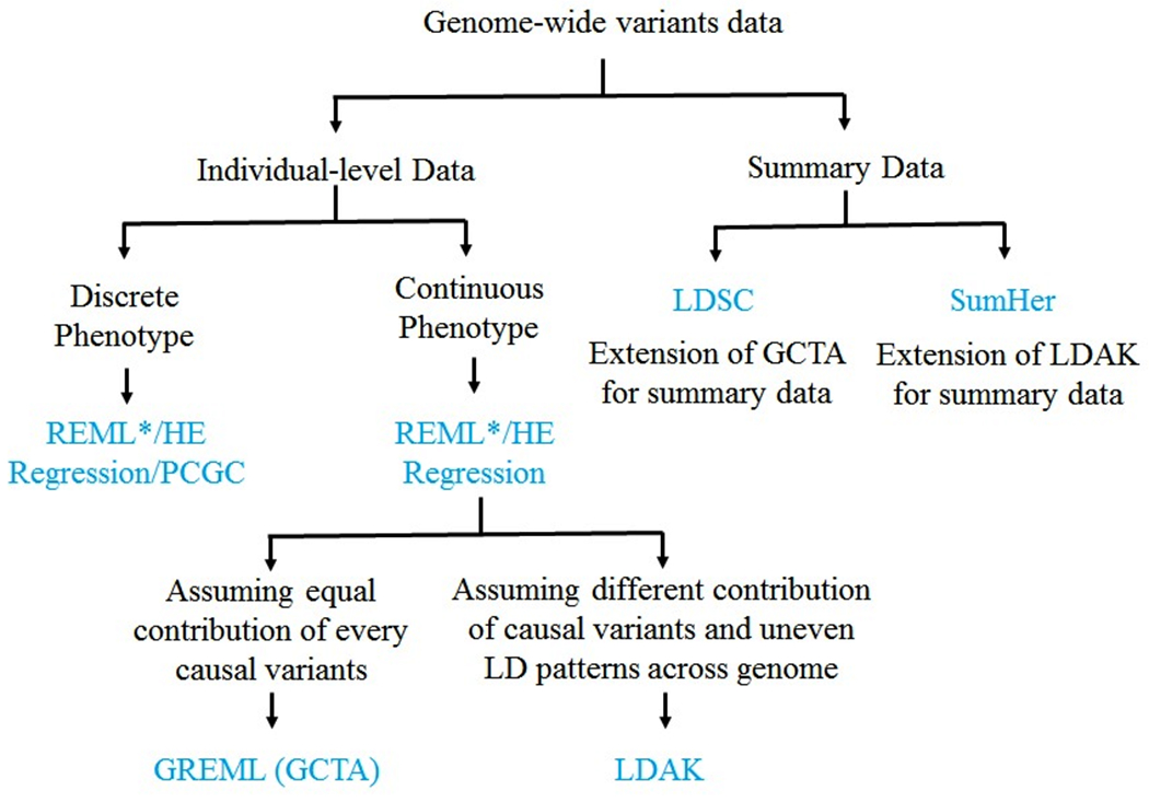
A summary of SNP-heritability estimation approaches utilizing individual-level genome-wide SNPs or summary results from previous GWAS. Such data could be generated through array, imputation and whole genome sequencing. REML - Restricted Maximum Likelihood Method; PCGC - Phenotype Correlation-Genotype Correlation; HE – Hasemann Elston Regression; GREML – Genomic Restricted Maximum Likelihood; LDAK – Linkage Disequilibrium adjusted Kinship LDSC – LD Score Regression.

The current review provides an updated summary of SNP-heritability estimation approaches utilizing either individual-level genome-wide data or summary results from previous GWAS. These approaches utilize a variety of methods such as Maximum Likelihood (ML) (Thompson, 1971; Visscher et al., 2006), Restricted Maximum Likelihood (REML) (Lee & van der Werf, 2006; Yang et al., 2010), Haseman-Elston (HE) Regression (Haseman & Elston, 1972; Sham & Purcell, 2001) and Phenotype Correlation-Genotype Correlation (PCGC)(Golan et al., 2014). REML is the most widely used method for individual-level genetic data and is employed in linear mixed model (LMM) to simultaneously estimate the contribution of fixed and random effects. Therefore, we focus here on the REML methods while discussing the approaches developed for individual-level genetic data. Likewise, we discuss LDSC (B. Bulik-Sullivan et al., 2015; B. K. Bulik-Sullivan et al., 2015) and SumHer (Speed & Balding, 2019) that utilize the regression method and REML respectively, to estimate SNP-heritability from GWAS summary results. We discuss each heritability estimation approach in the context of statistical basis, utility, advantages and limitations. We also provide stepwise protocols to apply commonly used approaches utilizing individual-level genetic data such as GCTA(Yang et al., 2010; Yang, Lee, et al., 2011), LDAK(Speed et al., 2017; Speed et al., 2012) and Threshold GREML (Zaitlen et al., 2013) as well as GWAS summary results such as LDSC (B. Bulik-Sullivan et al., 2015; B. K. Bulik-Sullivan et al., 2015) and SumHer (Speed & Balding, 2019). We present this review as a template to the researchers who need to estimate and use heritability in their research and as a reference to the geneticists who want to develop or extend heritability estimation approaches.

An overview of SNP-heritability estimation approaches

Genome-wide SNPs arrays and whole genome sequencing technologies have revolutionized many aspects of human genetics such as determination of genetic susceptibility and underlying mechanisms that increase risk of diseases, heritability and evolution of complex traits (Eichler et al., 2010; Visscher et al., 2008; Zaitlen & Kraft, 2012). Genome-wide association studies (GWAS) have discovered a multitude of genetic variants associated with various complex human traits and diseases (Buniello et al., 2019). However, variants derived from GWAS explain only a small proportion of phenotypic variance as compared to family studies leading to a major question of missing (hidden) heritability(Manolio et al., 2009). There are several possible reasons for missing heritability such as weak linkage disequilibrium (LD) between genotyped variants and ungenotyped causal variants, common variants with small effects that do not reach the canonical significance threshold (5 × 10⁻⁸) in GWAS, rare variants with large effects not captured by genotyping arrays, contribution of non-additive effects, gene environmental interactions and overestimation of narrow-sense heritability in pedigree-based studies due to shared environmental confounding (Eichler et al., 2010; Gibson, 2012; Manolio et al., 2009; Yang et al., 2017; G. Zhang, 2015). In last decade, several approaches have been developed that utilize genome-wide variations instead of only statistically significant variations to solve the problem of missing heritability of complex traits (B. K. Bulik-Sullivan et al., 2015; Speed & Balding, 2019; Speed et al., 2017; Speed et al., 2012; Yang, Lee, et al., 2011; Zaitlen et al., 2013). These approaches successfully explained a large proportion of phenotypic variance attributable to genome-wide SNPs for a variety of complex human traits and diseases. Unlike widely studied continuous traits such as anthropometric traits, behavioral traits and pre- and perinatal traits, dichotomous traits such as diseases are represented on a discrete scale (e.g., 0–1). Therefore, observed heritability on a risk scale is usually parameterized on an unobserved continuous liability scale so that the heritability is independent of disease prevalence(Falconer, 1965; Lee, Wray, Goddard, & Visscher, 2011; Tenesa & Haley, 2013; Yang et al., 2017). Here, we explain major advances in the approaches based on genome-wide SNPs data at individual or summary level with their advantages and limitations (Table 1).

Table 1: Summary of widely used approaches for the estimation of SNP-heritability:

Each approach is summarized on the basis of statistical assumptions and concept along with their advantages and limitations. u_i, p_i, w_i and ${\sigma }_i^2$ represent effect, MAF, weight and variance of SNP i, respectively; m represents number of SNPs used to create GRM or number of SNPs in summary statistics; s represents a subset of m present in a MAF bin, LD bin, genomic region or functional annotation; ${\mathrm{h}}_{\mathrm{g}}^2$ and ${\mathrm{h}}_{\mathrm{s}}^2$ represent SNP-heritability attributable to all SNPs used in the analysis and s subset of SNPs, respectively; α is a scaling factor, representing the influence of MAF on the variance of SNP effect.

Approach	Statistical Assumptions	Description	Advantages	Limitations
GREML-SC	(i) Normal distribution of SNP effects ${[\mathrm{u}}_{\mathrm{i}}\text{∼ N(0,}{\mathrm{h}}_{\mathrm{g}}^2/\mathrm{m}\left)\right]$, independent of LD and inversely proportional to MAF; ii) Polygenic model; iii) Uncorrelated Genetic and environmental components	i) Each SNP contributes equally to phenotypic variance i.e. ${\mathrm{\sigma }}_i^2={\mathrm{h}}_{\mathrm{g}}^2/\mathrm{m}$; ii) ${\widehat{\mathrm{h}}}_{\mathrm{S}\mathrm{N}\mathrm{P}}^2$ is dependent on the tagging of causal variants by the SNPs used to create the GRM.	First ever approach to estimate SNP-heritability using genome-wide data in unrelated individuals.	i) Highly dependent on LD among assayed and causal variants and biased to the extent at which the average LD among causal variants differ from the average LD among SNPs used to create GRM. ii) No flexibility of modelling uneven LD and MAF influence as compared to other contemporary approaches.
GREML-MS	Each GRM should follow same assumptions as GREML-SC. SNP effects follow the distribution ${[\mathrm{u}}_{\mathrm{i}}\text{∼ N(0,}{\sum }_{\mathrm{s}\mathrm{ϵ}\mathrm{m}}{\mathrm{h}}_{\mathrm{s}}^2/\mathrm{s}\left)\right]$	i) Multi-component GREML - multiple GRMs based on MAF bins are fitted simultaneously in the linear mixed model (LMM); ii) GRMs based on variety of bins such as chromosomes, genomic regions, functional annotation can be used.	Creating GRMs based on MAF bins can address the influence of MAF on SNP effects and variance. Since LD depends on MAF, GREML-MS can resolve uneven tagging of causal variants up to some extent.	i) Biased when LD structure of causal variants differ from that of the SNPs used to create the GRM; ii) Relatively large standard errors.
GREML-LDMS-R	Same as GREML-MS.	Multi-component GREML that bins SNPs by their MAF and regional LD.	Same as GREML-MS with additional advantage due to LD bins.	i) Similar to GREML-MS - if regional LD scores of causal variants differ from surrounding SNPs used to create GRM; ii) Relatively large standard errors.
GREML-LDMS-I	Same as GREML-MS.	Multi-component GREML that bins SNPs by their MAF and individual LD.	To date, best version of GREML (least biased approach) which can address the uneven tagging of causal variants and the influence of MAF on SNP effects.	i) Relatively large standard errors; ii) Usually runs 20 genetic components, therefore, difficult to constrain REML (0 < ĥ2 < 1), particularly when ĥ2 and/or sample size is small.
LDAK	Same as GREML-SC, except that i) contribution of causal variants are different depending on their LD with surrounding SNPs. LDAK allows modelling of uneven LD patterns across genome via weighing thinned SNPs differently and the influence of MAF on SNP effects. ${\mathrm{u}}_{\mathrm{i}}~\mathrm{N}\left(0,{\mathrm{\sigma }}_{\mathrm{i}}^2\right);$ ${\mathrm{\sigma }}_{\mathrm{i}}^2\propto {\mathrm{w}}_{\mathrm{i}}{\left[{\mathrm{p}}_{\mathrm{i}}\left(1-{\mathrm{p}}_{\mathrm{i}}\right)\right]}^{1+\mathrm{\alpha }}$	Developed to address the problem of uneven tagging of causal variants by the SNPs used to create GRM. Recommends using α = −0.25	Can correct uneven tagging of causal variants and allows modelling the influence of MAF on SNP effects	i) As biased as GREML-SC if assumptions aren’t met; ii) generally, larger standard errors as compared to GREML
LDAK-MS	Each GRM must hold same assumptions as LDAK.	Multi-component version of LDAK that bins SNPs by MAF.	Developed to give flexibility of fitting various models based on MAF bins	i) Less biased than LDAK, but more biased than GREML-LDMS; ii) Relatively large standard errors.
Threshold GREML	Estimates associated with the GRM without threshold are like GREML-SC. Variance attributable to the GRM with threshold represents (${\mathrm{h}}_{\mathrm{p}\mathrm{e}\mathrm{d}}^2\mathrm{ }-\mathrm{ }{\mathrm{h}}_{\mathrm{S}\mathrm{N}\mathrm{P}}^2$); where ${\mathrm{h}}_{\mathrm{p}\mathrm{e}\mathrm{d}}^2$ is the sum of variance attributable to both GRMs whereas ${\mathrm{h}}_{\mathrm{S}\mathrm{N}\mathrm{P}}^2$ is the variance attributable to the GRM without threshold.	Multi-component GREML with two GRMs: first GRM is created from all SNPs and second GRM is created by setting off-diagons below a set threshold to 0.	Generally useful in samples with extended genealogy.	It can be upwardly biased by shared environmental influences.
LD score (LDSC) regression	Polygenic model with normally distributed SNP effects. Statistical assumptions are same as GREML $[\mathrm{E}\left[{\mathrm{u}}_{\mathrm{i}}\right]=0;$ $\mathrm{v}\mathrm{a}\mathrm{r}\left({\mathrm{u}}_{\mathrm{i}}\right)=\mathrm{ }{\mathrm{h}}_{\mathrm{g}}^2/\mathrm{m}]$	Slope from regression of χ2 (from GWAS) on SNPs’ LD scores (from reference data) is used to estimate h2 attributable to the causal variants in LD with common SNPs present in GWAS summary result.	i) As compared to GREML, it requires only summary results instead of individual-level data; ii)Besides estimation of h2, LDSC can estimate genetic correlation with other traits; iii) LDSC was further extended to estimate h2 attributable to various functional annotations, cell and tissue types(Finucane et al., 2015); iv) Generally robust to confounding due to stratification and shared environmental effects; v) computationally efficient.	i) Estimated h2 is attributed to common causal variants only; ii) Underestimates h2 if the trait is not highly polygenic; iii) Biased estimates of h2 if reference population differs from the population used in GWAS.
SumHer	Basic idea is like LDSC with three differences - i) SumHer models inflation as multiplicative whereas LDSC models as additive; ii) Unlike LDSC, SumHer allows modelling uneven LD patterns across genome as well as influence of MAF on SNP effects s; iii) SumHer uses REML instead of regression to estimate SNP-heritability	An extension of the LDAK model that can estimate h2 from summary results of previous GWAS. It can also partition h2g attributable to different annotations.	Multiplicative modelling of inflation can be useful to avoid overcorrecting confounding in large GWAS; ii) SumHer has striking difference from LDSC in estimating h2 attributable to annotated regions.	Same as LDSC, except that SumHer apparently overestimates h2

Approaches utilizing individual-level genetic data

The fundamental idea behind the approaches developed for individual-level genome-wide data is to estimate the realized genetic relationship among individuals by using genome-wide variants and using this relationship matrix to estimate the genetic variance. Yang et. al. (2010) first utilized such approach to address the problem of missing heritability of human height. The study used 294,831 SNPs genotyped on 3,925 unrelated individuals to calculate realized genetic relatedness and fitted this relatedness matrix in LMM to estimate SNP-based narrow-sense heritability (${\widehat{\mathrm{h}}}_{\mathrm{S}\mathrm{N}\mathrm{P}}^2$) of human height. The results explained 45% of phenotypic variance in human height. Here, we discuss the most widely used SNP-heritability estimation approaches utilizing individual-level genetic data.

Genome-wide Complex Trait Analysis (GCTA)

One of the most popular software packages for estimating SNP-heritability using genome-wide data from unrelated individuals is Genome-wide Complex Trait Analysis (GCTA) that uses a genome-based restricted maximum likelihood (GREML) (Yang et al., 2010; Yang, Lee, et al., 2011) method. GCTA depends upon LD between genotyped variants and ungenotyped causal variants to estimate additive genetic variance in unrelated individuals.

The basic concept behind the method is to fit the effects of all the SNPs as random effects via an LMM. In this design, phenotype Y can be represented in simple equation form: $\mathrm{Y}=\mathrm{Z}\mathrm{u}+\mathrm{e}$; where Z is standardized genotype matrix (scaled genotypic values from unrelated individuals), u is the vector of random genetic effects with ${\mathrm{u}}_{\mathrm{i}}~\mathrm{N}(0,{\mathrm{\sigma }}_{\mathrm{i}}^2$) for SNP i and e is the vector of residual effects [e ~ N(0, I${\mathrm{\sigma }}_{\mathrm{e}}^2$)]. This model can be rewritten as $\mathrm{Y}=\mathrm{g}+\mathrm{e}$ where g = Zu is the additive genetic values of phenotype Y [g ~ N(0, $\mathrm{A}{\mathrm{\sigma }}_{\mathrm{g}}^2$)]; where A is genetic relatedness matrix (GRM) among unrelated individuals ($\mathrm{A}=\frac{\mathrm{Z}{\mathrm{Z}}^{\mathrm{T}}}{\mathrm{m}}$; where m is the number of variants) and ${\mathrm{\sigma }}_{\mathrm{g}}^2$ is additive genetic variance of all variants (${\mathrm{\sigma }}_{\mathrm{g}}^2=\mathrm{m}{\mathrm{\sigma }}_{\mathrm{i}}^2$). Similarly, phenotypic variance of Y can be expressed in terms of variance attributable to random (additive) effects (${\mathrm{\sigma }}_{\mathrm{g}}^2$) and residual effects (${\mathrm{\sigma }}_{\mathrm{e}}^2$).

$$\text{var}(\text{Y})=\text{A}{\mathrm{\sigma }}_{\mathrm{g}}^2+\text{I}{\mathrm{\sigma }}_{\mathrm{e}}^2$$

where A is GRM with each cell representing pair-wise genetic relatedness and I is identity matrix, assuming independence of environmental influence and no gene-gene or gene-environment interaction. For example, A_jk represents genetic relatedness between individuals j and k from m genotyped SNPs:

$${\text{A}}_{\mathrm{jk}}=\frac{1}{\text{m}}{\Sigma }_{\text{m}}\frac{({\text{x}}_{\text{ij}}-2{\text{p}}_{\text{i}})({\text{x}}_{\text{ik}}-2{\text{p}}_{\text{i}})}{2{\text{p}}_{\text{i}}(1-{\text{p}}_{\text{i}})}$$

where p_i is the minor allele frequency (MAF) and x_i is the genotype code of the SNP i (x_i = 0, 1, or 2).

A limitation of the GCTA approach is that it relies heavily on LD between assayed and causal variants (Speed et al., 2012; Zhu & Zhou, 2020). Therefore, it overestimates and underestimates the contribution of causal variants in high LD (strong LD between ungenotyped causal and genotyped variants) and low LD (weak LD between ungenotyped causal and genotyped variants) regions, respectively. In addition, genetic relatedness between a pair of individuals based on genotyped variants may not reflect genetic relatedness based on ungenotyped causal variants. If ungenotyped causal variants are in strong LD as compared to genotyped variants, heritability estimated using genotyped variants will be underestimated. GCTA suggests a uniform transformation of relatedness matrix [scaling the genotype matrix with 2p(1-p)⁻¹; where p is MAF]. Such scaling implies that effect sizes are inversely proportional to MAF and each causal variant contributes equally to the phenotypic variance. However, equal contribution of each causal variant to the phenotypic variance is not realistic due to uneven LD patterns across the genome. Additionally, assortative mating, epistasis and gene-environment interaction can bias heritability estimates by incorrectly allocating variance attributable due to these phenomena to additive genetic effects. Likewise, population structure (admixed population) can bias the estimation of heritability. This bias can usually be avoided by identifying population structure through principal component analysis (PCA) and eliminating outliers from the data or correcting for admixed samples in the analysis by including the first few PCs as fixed effects in the LMM.

Later, several other variants of GCTA based on MAF stratified variants (GCTA-MS), LD and MAF stratified variants (GCTA-LDMS) were developed to overcome these limitations (see protocol). These approaches facilitated not only partitioning of genetic variance in additive and non-additive components but also variance attributed to different chromosomes, genes and inter-genic regions, biological pathways and SNP functions (Yang et al., 2015; Yang, Manolio, et al., 2011). In addition, an approach was introduced to estimate SNP-heritability in individuals with close or extended relationships (Zaitlen et al., 2013). This approach essentially uses GREML with two GRMs; first GRM is created using all SNPs whereas a threshold is applied on the second GRM by setting off-diagonals < threshold to zero (see protocol). However, each approach has advantages and disadvantages (Table 1).

Linkage Disequilibrium adjusted Kinships (LDAK)

Speed et al. (2012) developed a method (Linkage Disequilibrium adjusted Kinships - LDAK) to overcome the bias arising from ungenotyped causal variants in regions of high or low LD. Yang et. al. suggested a uniform scaling of the SNP-based kinship matrix [2p(1-p)⁻¹; where p is MAF]. This transformation adjusts for the average bias caused by variable LD leading to uneven tagging of ungenotyped causal SNPs across genome, however, it depends upon the MAF spectrum of the causal SNPs which is generally not known. In contrast, LDAK suggests modification of the GRM according to local LD - contribution of the SNPs to the genetic similarity between a pair of individuals is weighted according to the LD with their neighboring SNPs. Estimating heritability using genetic similarity adjusted for Local LD reduces the potential bias and increases the precision of the heritability estimate.

Reanalysis of the height data with LD-adjusted GRM showed a slight change in the estimated SNP-based heritability (${\widehat{\mathrm{h}}}_{\mathrm{S}\mathrm{N}\mathrm{P}}^2$), suggesting that the underestimation of h² in low-LD regions was balanced by overestimation of h² in high-LD regions. However, approximately a quarter increase in ${\widehat{\mathrm{h}}}_{\mathrm{S}\mathrm{N}\mathrm{P}}^2$ of hypertension and type I diabetes using LDAK as compared to GCTA suggested that causal SNPs were poorly tagged by genotyped SNPs i.e. causal SNPs had lower MAF than genotyped SNPs and a uniform transformation didn’t represent these LD patterns(Speed et al., 2012). In contrast, nearly one tenth decrease in ${\widehat{\mathrm{h}}}_{\mathrm{S}\mathrm{N}\mathrm{P}}^2$ of rheumatoid arthritis suggested that causal SNPs had higher MAF as compared to genotyped SNPs (Speed et al., 2012). Further, LDAK was used for imputed data across 19 human traits to develop a model for accurately describing the variation in ${\widehat{\mathrm{h}}}_{\mathrm{S}\mathrm{N}\mathrm{P}}^2$ with MAF, LD and genotype certainty. Improved model led to on average 43% (S.D. 3%) higher ${\widehat{\mathrm{h}}}_{\mathrm{S}\mathrm{N}\mathrm{P}}^2$ than those obtained from GREML and 25% (S.D. 2%) higher ${\widehat{\mathrm{h}}}_{\mathrm{S}\mathrm{N}\mathrm{P}}^2$ than those from GREML-LDMS (Speed et al., 2017).

Like GCTA, LDAK estimates are highly sensitive to MAF of causal variants, population stratification and SNP data type [arrays, imputed or Whole Genome Sequence (WGS)]. In addition, as LD is a function of MAF, the weighting strategy in LDAK can introduce MAF bias because it gives more weight to SNPs with lower MAF. An analysis using all SNPs from WGS data showed that LDAK weighted SNPs inversely proportional to their LD which resulted in near-zero weights for common SNPs and very high weights for rare SNPs. This led to underestimated ${\mathrm{h}}_{\mathrm{S}\mathrm{N}\mathrm{P}}^2$ for common variants and overestimated ${\mathrm{h}}_{\mathrm{S}\mathrm{N}\mathrm{P}}^2$ for rare variants. The LDAK-induced MAF bias can be substantial, especially when there are several rare variants, leading to an inflated estimate of ${\mathrm{h}}_{\mathrm{S}\mathrm{N}\mathrm{P}}^2$(Yang et al., 2017). LDAK assumes that the variance explained by rare variants is very large in comparison to that explained by common variants which predicts that the power to detect rare variants would be higher than that to detect common variants in the same order. This prediction is not consistent with empirical results in the cases of human height, schizophrenia, and type 2 diabetes (Yang et al., 2017).

Approaches utilizing summary results from previous GWAS

We discussed the approaches to estimate ${\mathrm{h}}_{\mathrm{S}\mathrm{N}\mathrm{P}}^2$ from individual-level genome-wide SNPs data, however, availability of such data with relevant phenotype information is often limited. Therefore, other approaches were developed that utilize summary results of GWAS (estimated SNP effects and their standard errors for hundreds of thousands of SNPs analyzed in a study) instead of per-individual genome-wide information.

LD Score (LDSC) Regression

In GWAS, the deviation of observed χ² test statistic for a SNP from its expected value under the null hypothesis (no association) is a function of LD between a target SNP and underlying causal variants (Yang et al., 2017). Therefore, ${\mathrm{h}}_{\mathrm{S}\mathrm{N}\mathrm{P}}^2$ can be directly estimated from the summary results by regressing the observed χ² test statistic against LD score of genome-wide SNPs. This is the basic principle of the LD Score regression approach (LDSC) (B. Bulik-Sullivan et al., 2015; B. K. Bulik-Sullivan et al., 2015). Under the polygenic model, average variance explained by each SNP is ${\mathrm{h}}_{\mathrm{S}\mathrm{N}\mathrm{P}}^2$/m, where m and ${\mathrm{h}}_{\mathrm{S}\mathrm{N}\mathrm{P}}^2$ are number of SNPs and total variance attributable to all SNPs in the summary data, respectively. Therefore, the expected χ2 can be represented as $\mathrm{E}\left(\mathrm{\chi }2|{\mathrm{l}}_{\mathrm{i}}\right)=1\mathrm{ }+\mathrm{ }\frac{{\mathrm{h}}_{\mathrm{S}\mathrm{N}\mathrm{P}}^2\mathrm{N}}{\mathrm{m}}{\mathrm{l}}_{\mathrm{i}}$ for SNP i, where N is number of individuals and l_i is the sum of LD r² values between SNP i and all SNPs (including itself). This approach requires only summary data from GWAS because LD scores can be estimated in a reference population (for example, the 1000 Genomes Project). Besides LD between the target SNP and the underlying causal variants, cryptic relatedness/population stratification can also inflate the expected χ2 test statistics. Therefore, an extra term (a) can be included in the model for confounding biases: $\mathrm{E}\left(\mathrm{\chi }2|{\mathrm{l}}_{\mathrm{i}}\right)=1+\mathrm{N}\mathrm{a}+\mathrm{ }\frac{{\mathrm{h}}_{\mathrm{S}\mathrm{N}\mathrm{P}}^2\mathrm{N}}{\mathrm{m}}{\mathrm{l}}_{\mathrm{i}}$. Regression of the observed χ2 test statistics against LD scores of genome wide SNPs [$\mathrm{E}\left(\mathrm{\chi }2|{\mathrm{l}}_{\mathrm{i}}\right)={\mathrm{b}}_0+{\mathrm{b}}_1{\mathrm{l}}_{\mathrm{i}}$] can not only detect an inflation due to confounding factors such as population stratification (b₀ >1 represents confounding bias) but also estimate ${\mathrm{h}}_{\mathrm{S}\mathrm{N}\mathrm{P}}^2\mathrm{ }({\widehat{\mathrm{h}}}_{\mathrm{S}\mathrm{N}\mathrm{P}}^2=\frac{{\mathrm{b}}_1\mathrm{m}}{\mathrm{N}}$).

Like GCTA, LDSC has also been extended to estimate genetic correlation (r_g) between traits using summary results. Genetic correlation can be defined as genetic covariance normalized by SNP-heritability [$r_g=\frac{{\rho }_{xy}}{{\sigma }_x{\sigma }_y}\approx \frac{{\mathrm{h}}_{xy}^2}{\sqrt{{\mathrm{h}}_x^2{\mathrm{h}}_y^2}}$], where ${\rho }_{xy},\mathrm{ }{\sigma }_x$, and ${\sigma }_y$ represent genetic covariance between trait x and y, square root of genetic variance of x and y respectively that can be approximated as additive genetic covariance between x and y (${\mathrm{h}}_{xy}^2$) and square roots of SNP-based narrow-sense heritability of x (${\mathrm{h}}_x^2$) and y (${\mathrm{h}}_y^2$). Unlike pedigree-based methods, bivariate (multivariate) GREML, an extension of GREML estimates genetic correlations between traits (or diseases) in unrelated individuals, for example two independent studies. While LDSC also allows the traits sought for genetic correlation to be measured on different set of samples, major advantage of LDSC is that it requires only summary statistics. Calculations for genetic correlation are quite similar to heritability estimations via LDSC. χ² statistics for a single study is replaced with the product of z-scores from two studies of traits with non-zero genetic correlation. An expected value of product of z-scores from two studies, study 1 and 2, based on SNP i can be expressed as $\mathrm{E}\left({\mathrm{z}}_{1\mathrm{i}}{\mathrm{z}}_{2\mathrm{i}}\right)=\frac{\mathrm{\rho }{\mathrm{N}}_{\mathrm{S}}}{\sqrt{{\mathrm{N}}_1{\mathrm{N}}_2}}+\frac{\sqrt{{\mathrm{N}}_1{\mathrm{N}}_2}{\mathrm{\rho }}_{\mathrm{g}}}{\mathrm{m}}{\mathrm{l}}_{\mathrm{i}}$, where N₁ and N₂ are sample sizes from study 1 and 2, N_S is the number of individuals included in both studies, ρ is the phenotypic correlation among the N_S overlapping samples, ${\mathrm{\rho }}_{\mathrm{g}}$ is the genetic covariance between trait 1 and 2 and l_i is the sum of LD r² values between SNP i and all SNPs (including itself). Hence, ${\mathrm{\rho }}_{\mathrm{g}}$ can be estimated by regressing the product of z-scores from two studies (${\mathrm{z}}_1{\mathrm{z}}_2$) on LD r² values (${\widehat{\mathrm{\rho }}}_{\mathrm{g}}=\frac{{\mathrm{b}}_1\mathrm{m}}{\sqrt{{\mathrm{N}}_1{\mathrm{N}}_2}}$). If study 1 and study 2 are the same study, then genetic covariance between a trait and itself is the estimate of heritability (${\widehat{\mathrm{h}}}_{\mathrm{S}\mathrm{N}\mathrm{P}}^2$), and χ²=z². Once genetic covariance (${\mathrm{\rho }}_{\mathrm{g}}$) is estimated, genetic correlation (r_g) can be estimated in the same way as with GCTA. As compared to GCTA, LDSC provides great flexibility to estimate r_g between any two GWAS data sets.

A major advantage of LDSC is that it is faster than individual-based approaches and its computing time does not scale up with sample size. LDSC only requires summary data, which allows the reanalysis of summary data available from published meta-analyses. The LD score regression intercept can be used to estimate population stratification. Since summary results are available usually only for common variants, LDSC is limited in estimation of the variance explained by rare variants even with imputed or WGS data and it is more sensitive to the genetic architecture of a trait. The estimates using LDSC depend on the LD scores and thereby, the reference population in which LD scores were calculated. If there is a mismatch between the LD Scores from the reference population and the target population used for GWAS, then LD Score regression can be biased. A previous study showed that ${\widehat{\mathrm{h}}}_{\mathrm{S}\mathrm{N}\mathrm{P}}^2$ measures from LDSC are consistently smaller than those from GREML in the same data set, which is likely due to errors in LD scores estimated from the reference population (LDSC recommends using LD scores from HapMap 3 SNPs in the 1000 Genomes Project) (Ni, Moser, Schizophrenia Working Group of the Psychiatric Genomics, Wray, & Lee, 2018).

LD Score Regression has been frequently applied to summary statistics from GWAS - to estimate the SNP-heritability of a trait, average bias due to confounding, heritability enrichments of SNP categories, and genetic correlation between a pair of traits. Like GCTA, LDSC also assumes that all causal variants contribute equally to the phenotypic variance and therefore provides equal weight to each SNP. Although this model is widely used in statistical genetics, it usually underestimates the average ${\widehat{\mathrm{h}}}_{\mathrm{S}\mathrm{N}\mathrm{P}}^2$ in regions of high LD (due to multiple tagging of causal variants). LDSC tends to over-estimate confounding bias, under-estimate SNP heritability and produce exaggerated estimates of enrichments, due to misspecification of heritability model(Speed & Balding, 2019).

SumHer

Speed et. al. (2019) proposed an approach (SumHer) to overcome the limitations of LDSC(Speed & Balding, 2019; Speed et al., 2020). The basic idea behind SumHer is that SNP heritability (e.g. ${\widehat{\mathrm{h}}}_{\mathrm{i}}^2$ for SNP i) varies across the genome and therefore, $\mathrm{E}\left({\widehat{\mathrm{h}}}_{\mathrm{i}}^2\right)\propto {\mathrm{q}}_{\mathrm{i}}={\left[{\mathrm{p}}_{\mathrm{i}}\left(1-{\mathrm{p}}_{\mathrm{i}}\right)\right]}^{1+\mathrm{\alpha }}{\mathrm{w}}_{\mathrm{i}}$; where ${\mathrm{p}}_{\mathrm{i}}$ is MAF of SNP i, w_i is the weight calculated for SNP i based on local LD and $\alpha$ is a constant (like LDAK, SumHer chooses $\alpha = -0.25$ by default)]. The main difference between LDSC and SumHer is that unlike LDSC (it assumes all q_j are same; q_i=1), SumHer allows users to choose any heritability model i.e., the user can specify arbitrary values for q_i. As compared to additive modelling of inflation in LDSC, SumHer models inflation of test statistics multiplicatively. A recent analysis of 24 large-scale GWAS using the recommended model in SumHer showed that these studies were inclined to over-correct for confounding, which reduced the discovery of genome-wide significant loci by about a quarter(Speed & Balding, 2019). Heritability estimate enrichment analyses using LDSC concluded that heritability is highly concentrated in specific functional categories. For example, an analysis across 17 diseases showed that conserved regions contribute 35% of SNP heritability, indicating that they were 13-fold enriched for casual variants. By contrast, analyses across 24 traits using SumHer finds that none of the categories have enrichment above twofold(Speed & Balding, 2019).

SumHer proposes a solution to unequal contribution of ${\widehat{\mathrm{h}}}^2$ per SNP due to differential LD pattern, overestimation of confounding due to population stratification and exaggerated heritability enrichment due to misspecification of the heritability model. However, it also suffers from limitations in common with LDSC. It is not known yet how well the SumHer heritability model would fit while estimating variance attributable to rare variants. Like LDSC, heritability estimates from SumHer depend on LD scores from reference samples indicating a mismatch in LD scores from reference samples and GWAS samples would result in biased estimation of ${\widehat{\mathrm{h}}}^2$.

Step-by-step guide for SNP-heritability estimation

Here, we provide a stepwise guide to estimate SNP-heritability using various approaches. For illustration purposes, we use individual-level genetic data and summary results from previous GWAS to estimate SNP-heritability of height and BMI. Individual-level genetic data from The Northern Finnish Birth Cohort (NFBC; 1966) consists of several metabolic trait measurements in 5402 individuals (Sabatti et al., 2009), genotyped for 364,580 SNPs using Illumina HumanCNV370-Quadv3_C platform. Likewise, we use summary results from meta-analysis of height and BMI using UK Biobank and GIANT GWAS (2018)(Yengo et al., 2018).

The NFBC dataset is available through DbGaP authorized access. This data is for general research use - i.e., use of the data is limited only by the terms of the model Data Use Certification. There is no limitation in the usage of the genomic results outside the study for which they were originally consented. Summary results from GIANT consortium are publicly available and can be accessed without restriction.

Although not an integral part of the protocol, we also provide a brief overview of widely used quality control procedure for phenotype and genotype data. Current approaches, developed for SNP-heritability estimation can also be used for various other purposes for example, estimation of genetic correlation, confounding due to population structure and cryptic relationship, gene enrichment analysis. However, we provide protocols only for the SNP-heritability estimation to align with the focus of the current review.

Resources

Before starting the estimation of SNP-heritability, it is necessary to install appropriate software, assemble the data files – input genotype (usually, plink format is preferred; if genotypes are present in variant call format (vcf) file, it can be converted to plink format for further analyses), phenotype (phenotype file should have at least three columns in the order – family id, individual id and phenotypic values) and summary results (usually, contains an identifier/SNP id, effect allele, other allele, sample size, p value and summary statistics) and download pre-calculated tagging (LD score) information from reference population (e.g., 1,000 genomes database, UK Biobank database). Reference population used for LD scores should be ancestrally similar to the GWAS samples. Similarly, we should be cautious while using summary results from previous GWAS and use the large studies with rigorous quality control.

Hardware:

Any laptop/computer with 4 cores and 8–16 GB RAM is sufficient for most of the analyses in a reasonable time(Yang, Lee, et al., 2011).

Operating System:

Linux-based operating system such as Ubuntu, Fedora etc.

Quality Control of phenotype and genotype data

A detailed description of quality control for genome-wide analysis can be found elsewhere (Truong et al., 2022; Turner et al., 2011; Weale, 2010). Here, we briefly summarize the routinely used quality control procedures. In general, quality control of phenotypes depends on the research question, trait type (discrete or continuous) and other phenotypes/covariates available in the dataset. R (R. C. Team, 2020)/R-Studio (R. Team, 2019) (https://www.R-project.org) is a well-established platform for phenotype quality control. The first step is to select a key phenotype in a given dataset with multiple phenotypes, followed by summarizing the data. A density plot for continuous traits and bar plot for discrete traits can provide a rough idea about phenotype distribution and outliers. As normal distribution of variables is one of the assumptions in commonly used analyses, removing outliers (mean ±4*S.D.) is a common practice to attain normality in the dataset. However, one should be cautious while removing outliers and should choose this option only when alternative approaches such as data transformation (log or exponential) or adjusting with other covariates do not work. Phenotype data can be supplied to linear models either adjusted for the covariates or without adjusting for covariates where covariates can be supplied separately into the model.

Quality control of the genotype file is performed based on individuals and markers. PLINK (Chang et al., 2015; Purcell et al., 2007) (https://www.cog-genomics.org/plink/1.9) and R/R-Studio (R. Team, 2019; R. C. Team, 2020) (https://www.R-project.org) are routinely used for genotype quality control and plotting various quality measures, respectively. In general, individuals are filtered on the basis of genotype missing rate, average heterozygosity (inbreeding), inconsistency between biological and reported sex and Mendelian errors (if pedigree information is available). Similarly, markers are filtered on the basis of call rate, minor allele frequency (MAF) and Hardy-Weinberg equilibrium (HWE). In addition, heritability estimation methods assume a homogeneous population, therefore it is advisable to check for population stratification and remove outliers using principal component analysis (PCA) or Multi-dimensional scaling (MDS) based on the set of markers in the genome that are independent.

We performed quality control procedure for NFBC dataset as mentioned above. After careful examination of density plot of height and BMI, 33 samples were removed from the analysis. Phenotypes were adjusted for sex before fitting into LMM. Similarly, genotype data was controlled for individual and marker quality. Individuals were examined and excluded on the basis of genotype missing rate > 5%, average heterozygosity ± 4*S.D. and inconsistency between reported and biological sex whereas SNPs were examined and excluded on the basis of call rate < 95%, MAF > 1% and HWE with p < 1.0E-6. After genotype and phenotype quality control, 5,348 individuals genotyped on 324,851 autosomal SNPs with available phenotype information remained for SNP-heritability estimation analyses.

Protocols

Assuming that genotype and phenotype files are pre-processed for quality control, we provide below protocols to run SNP-heritability analyses using different heritability estimation approaches. We believe that these protocols will facilitate the readers to estimate SNP-heritability (${\mathrm{h}}_{\mathrm{S}\mathrm{N}\mathrm{P}}^2$) using individual-level data and summary statistics.

BASIC PROTOCOL 1: GREML (GCTA)

GREML protocol can be broadly categorized into three steps – 1) create genetic relatedness matrix (GRM); 2) remove one of the cryptically related individual pairs; 3) run restricted maximum likelihood (REML). GCTA allows multi-threading that can be enabled by using flag --thread-num or –threads.

Software and files needed for GREML

Software

GCTA(Yang et al., 2010; Yang, Lee, et al., 2011) (https://yanglab.westlake.edu.cn/software/gcta/#Download)

Data file

The Northern Finland Birth Cohort(Sabatti et al., 2009)

(https://www.ncbi.nlm.nih.gov/projects/gap/cgi-bin/study.cgi?study_id=phs000276.v2.p1)

1). Create GRM using plink format files (test.bed, test.bim and test.fam)

Depending upon the requirement of analysis, GRMs can be created in different ways such as using only autosomes, each chromosome separately, using X-chromosome alone or using a subset of SNPs.

a). Using autosomes only

gcta64 --bfile test --autosome --make-grm-bin --out test_grm --thread-num 4;

b). Based on each chromosome separately

gcta64 --bfile test --chr 1 --make-grm-bin --out test_grm_chr1 --thread-num 4;

gcta64 --bfile test --chr 2 --make-grm-bin --out test_grm_chr2 --thread-num 4;

…

gcta64 --bfile test --chr 22 --make-grm-bin --out test_grm_chr22 --thread-num 4;

c). Using X chromosome

gcta64 --bfile test --make-grm-xchr --out test_grm_xchr --thread-num 4;

d). Create GRM with a subset of SNPs (test_snplist.txt – one SNP in a line)

gcta64 --bfile test --extract test_snplist --make-grm-bin --out test_grm_subset --thread-num 4;

2). Remove one individual from each cryptically related pair using kinship coefficient cutoff (0.05)

gcta64 --grm test_grm --grm-cutoff 0.05 --make-grm-bin -–out test_grm_0.05 --thread-num 4;

3). Run REML with kinship matrix (test_grm_0.05.grm.bin, test_grm_0.05.grm.N.bin and test_grm_0.05.grm.id) and phenotype file (test.phen)

gcta64 --grm test_grm_0.05 --pheno test.phen --reml --out test_greml --thread-num 4;

The phenotype file typically has three columns – Family ID, Individual ID and Phenotype. However, more than one phenotype can also be provided and assigned to a specific column (phenotype) for ${\mathrm{h}}_{\mathrm{S}\mathrm{N}\mathrm{P}}^2$ estimation by providing an additional option –mpheno [(column-number) – 2] in the above command.

REML can also be run in various alternative ways such as using GRMs created by a subset of SNPs, using multiple GRMs, adjusting for covariates and using discrete outcomes e.g. case-control status in phenotype file.

a). Run REML using GRM created by a subset of SNPs (test_grm_subset.grm.bin, test_grm_subset.grm.N.bin and test_grm_subset.grm.id)

gcta64 --grm test_grm_subset --keep test_grm_0.05.grm.id --pheno test.phen --reml --out test_greml_subset --thread-num 4;

b). Run REML using multiple GRMs (grm_chrs.txt is a text file with list of GRM names – one GRM name in a line)

gcta64 --mgrm grm_chrs.txt --pheno test.phen --reml --out test_greml_chrs --thread-num 4;

c). Adjust for covariates (--covar and –qcovar for discrete and continuous covariates, respectively)

gcta64 --reml --grm test_grm_0.05 --pheno test.phen --covar sex.txt --qcovar PCs.txt --out test_greml_adj --thread-num 4;

sex.txt is a list of individuals’ sexes (discrete variable) and PCs.txt is file with first 10–20 principal components (continuous variable). Similar to the phenotype files, covariate files also have first two columns as family id and individual id followed by covariate columns.

d). Run REML for case control data (test_cc.phen – phenotype file with case-control information)

Let’s assume prevalence of disease is 0.1 in the general population. Option --prevalence is used to specify the disease prevalence and transformation of ${\widehat{\mathrm{h}}}_{\mathrm{S}\mathrm{N}\mathrm{P}}^2$ from observed discrete (0–1) scale to unobserved continuous liability scale.

gcta64 --reml --grm test_grm_0.05 --pheno test_cc.phen --prevalence 0.1 --out test_greml_cc --thread-num 4;

Note: Usually, GCTA runs reml in a constrained manner such that 0 < ${\widehat{\mathrm{h}}}^2$ < 1. If there are multiple matrices each with small contribution to ${\widehat{\mathrm{h}}}^2$, one or more random effects may hit the boundary. REML stops if more than half of the total components hit the boundary. To avoid such situation, --reml-no-constrain can be used to run REML in an unconstrained manner.

ALTERNATE PROTOCOL 1: Stratified-GREML

As seen in the previous example, SNP-heritability attributable to each chromosome can be estimated by simultaneously fitting GRMs based on each chromosome in to REML. Similarly, GREML can be run in various other stratified ways, for example, using GRMs created by a subset of SNPs stratified by either minor allele frequency (MAF) bins alone or both linkage disequilibrium (LD) and MAF bins. These variations of GREML were developed to adjust for the influence of MAF and local LD on the estimated SNP-heritability and known as GREML-MAF Stratified (GREML-MS) and GREML-LD and MAF Stratified (GEML-LDMS) approach, respectively. Like original GREML, stratified GREML is also performed in three major steps – 1) create GRM, 2) remove one of the cryptically related individual pairs and 3) run REML. However, GREML-LDMS includes an additional step - calculation of LD scores (summation of r² values between a SNP and all SNPs in a given genomic region), prior to creating GRMs. It is noteworthy that multiple GRMs are created and fitted in REML based on the stratification criteria in stratified GREML.

Software and files needed for Stratified-GREML

Software

GCTA(Yang et al., 2010; Yang, Lee, et al., 2011) (https://yanglab.westlake.edu.cn/software/gcta/#Download)

R/R-Studio(R. Team, 2019; R. C. Team, 2020) (https://www.R-project.org)

Data file

The Northern Finland Birth Cohort(Sabatti et al., 2009)

(https://www.ncbi.nlm.nih.gov/projects/gap/cgi-bin/study.cgi?study_id=phs000276.v2.p1)

GREML-MS (Based on MAF bins only)

1a. Create GRMs

gcta64 --bfile test --autosome --maf 0.01 --max-maf 0.1 --make-grm-bin --out test_maf0.1_grm --thread-num 4;

gcta64 --bfile test --autosome --maf 0.1 --max-maf 0.2 --make-grm-bin --out test_maf0.2_grm --thread-num 4;

gcta64 --bfile test --autosome --maf 0.4 --max-maf 0.5 --make-grm-bin --out test_maf0.5_grm --thread-num 4;

2a. Remove one of the cryptically related individual pairs:

REML can be run with unrelated individuals by adding a flag --keep [list of individuals with kinship coefficient < 0.05]. A list of individuals with kinship coefficient less than a set threshold can be created using the protocol provided in GCTA. Alternatively, test_grm_0.05.grm.id file created in the GREML protocol can directly be used. It is noteworthy that stratified REML analysis is performed with multiple GRMs listed in a text file (one GRM name in a line).

3a. Run REML

gcta64 --mgrm greml_ms_grm_list.txt --pheno test.phen --reml --out test_greml_ms;

GREML-LDMS (Based on LD and MAF bins)

1b. Calculate LD scores

LD scores are calculated using option --ld-score-region [window size]. GCTA uses default window size of 200Kb with 100Kb overlapping regions between two segments.

gcta64 --bfile test --autosome --ld-score-region 200 --out test_ld --thread-num 4;

Import output of above command (test_ld.score.ld) to R and create quartiles based on either ldscore_SNP or ldscore_region. Save SNPs corresponding to each quartile as test_ld_q*.txt, where * is 1/2/3/4. Different bins are created on the basis of LD score quartiles and MAF ranges. For example, SNPs within each MAF range such as 0.01 < MAF ≤ 0.1, 0.1 < MAF ≤ 0.2, , 0.2 < MAF ≤ 0.3, , 0.3 < MAF ≤ 0.4 and 0.4 < MAF ≤ 0.5 can be binned on the basis of quartiles of regional or SNP LD scores.

2b. Create GRM

for i in $(seq 1 4); do

  gcta64 --bfile test --autosome --extract test_ld_q${i}.txt --maf 0.01 --max-maf 0.1 --make-grm-bin --out test_q${i}_maf0.1_grm --thread-num 4;

done;

for i in $(seq 1 4); do

  gcta64 --bfile test --autosome --extract test_ld_q${i}.txt --maf 0.1 --max-maf 0.2 --make-grm-bin --out test_q${i}_maf0.2_grm --thread-num 4;

done;

…

for i in $(seq 1 4); do

  gcta64 --bfile test --autosome --extract test_ld_q${i}.txt --maf 0.4 --max-maf 0.5 --make-grm-bin --out test_q${i}_maf0.5_grm --thread-num 4;

done;

3b. Remove one of the cryptically related individual pairs:

One individual from the cryptically related pairs can be removed using the command provided in GCTA protocol. Alternatively, already filtered list of unrelated individuals can be used as in GREML-MS.

4b. Run REML

gcta64 --mgrm greml_ldms_grm_list.txt --pheno test.phen --reml --out test_greml_ldms;

BASIC PROTOCOL 2: LDAK

LDAK protocol can be divided into five steps – 1) Thinning of SNPs; 2) calculate weights of thinned SNPs based on the pair-wise LD with all nearby SNPs in a bin (e.g., 100 kb); 3) create kinship matrix; 4) remove one of the cryptically related individual pairs; 5) run REML. In the following protocols, we use default setting of α = −0.25; the user may change this depending on the desired model. Like GCTA, LDAK also allows multi-threading for most of the analyses which can be enabled by using option –max-threads.

Software and files needed for LDAK

Software

LDAK(Speed et al., 2017; Speed et al., 2012) (http://dougspeed.com/downloads) for the first-time users and (http://dougspeed.com/downloads2) for the returning users

Data file

The Northern Finland Birth Cohort(Sabatti et al., 2009)

(https://www.ncbi.nlm.nih.gov/projects/gap/cgi-bin/study.cgi?study_id=phs000276.v2.p1)

1). Thinning of SNPs

Thinning of SNPs means removing one of the SNP pairs that are in strong LD with each other from the analysis. LDAK uses r² = 0.98 and 100Kb window size as default values.

ldak5.1.linux --thin --bfile test --chr AUTO --window-prune .98 --window-kb 100;

awk ‘{print $1, 1}’ thin.in > weights.thin;

All thinned SNPs in the file ‘weights.thin’ are assigned equal weight i.e. 1 and are used for calculation of kinship matrix using LDAK-Thin model.

2). Calculate weights of thinned SNPs

All the thinned SNPs are weighted equally for the LDAK-Thin model, whereas variant specific weights are calculated for LDAK model. Prior to calculation of variant specific weights, LDAK cuts the thinned SNPs into multiple sections. We save these sections and corresponding SNP weights for each chromosome in a sub-directory ./sections/section${j}, where j represents chromosome number 1–22.

awk ‘NR==FNR{x[$1] = $0; next} $2 in x{print $1 “:” $2 “:” $4 “:” $6 “:” $5}’ thin.in test.bim > extend_thin.in;

awk ‘NR==FNR{x[$1] = $0; next} $2 in x{print $1 “:” $2 “:” $4 “:” $6 “:” $5}’ thin.out test.bim > extend_thin.out;

for j in $(seq 1 22); do

  mkdir -p ./sections/sections$j/;

  awk -v var=$j ‘{split($1, a, “:”); if(a[1] == var) print a[2]}’ extend_thin.in > ./sections/sections$j/thin.in;

done;

for j in $(seq 1 22); do

  awk -v var=$j ‘{split($1, a, “:”); if(a[1] == var) print a[2]}’ extend_thin.out > ./sections/sections$j/thin.out;

done

for j in $(seq 1 22); do

  ldak5.1.linux --cut-weights ./sections/sections$j --bfile test --chr $j --no-thin DONE --max-threads 4;

  ldak5.1.linux --calc-weights-all ./sections/sections$j --bfile test --chr $j --max-threads 4;

done;

cat ./sections/sections{1..22}/weights.short > ./sections/weights.short;

Thinned SNPs in the file ‘weights.short’ have SNP-specific weights and are used to calculate kinship matrix using LDAK model. weights.short usually has a smaller number of SNPs than initially thinned SNPs because many of the thinned SNPs have zero weight and are not included in the calculation of kinship matrix.

3). Create kinship matrix

a). Calculate Kinship matrix using same weight for all thinned SNPs (LDAK-Thin model)

ldak5.1.linux --calc-kins-direct test_grm_ldak_thin --bfile test --chr AUTO --weights weights.thin --power −0.25 --max-threads 4;

b). Calculate Kinship matrix using SNP specific weights (LDAK Model)

ldak5.1.linux --calc-kins-direct test_grm_ldak --bfile test --chr AUTO --weights ./sections/weights.short --power −0.25 --max-threads 4;

4). Remove one of the cryptically related individual pairs

a). LDAK-Thin model

ldak5.1.linux –filter test_ldak_thin_0.05 --grm test_grm_ldak_thin --max-rel 0.05 --max-threads 4;

b). LDAK model

ldak5.1.linux –filter test_ldak_0.05 --grm test_grm_ldak --max-rel 0.05 --max-threads 4;

The above commands produce two files - test_ldak_thin_0.05.keep and test_ldak_thin_0.05.lose or test_ldak_0.05.keep and test_ldak_0.05.lose depending on the selected model. While running REML we can use .keep file by adding a flag --keep [keep-file]. However, we use the same set of individuals (test_grm_0.05) as used in GCTA approach to maintain uniformity across different approaches.

5). Run REML

a). LDAK-Thin model

ldak5.1.linux --reml test_ldak_thin --pheno test.phen --pheno --grm test_grm_ldak_thin --keep test_grm_0.05.grm.id --constrain YES --max-threads 4;

b). LDAK model

ldak5.1.linux --reml test_ldak --pheno test.phen --pheno --grm test_grm_ldak --keep test_grm_0.05.grm.id --constrain YES --max-threads 4;

ALTERNATE PROTOCOL 2: Stratified-LADK

A stratified version of LDAK can be run using already calculated weights of thinned SNPs (see LDAK protocol). Unlike, GCTA, LDAK does not allow --min-maf or --max-maf option along with --calc-kins-direct. Therefore, markers based on MAF bins should be extracted from ‘test.bim’ files and the list should be used to extract the set of markers while creating kinship matrix (--extract list-of-SNPs.txt). Since, we are using pre-computed weights and advise one uses already pruned set of individuals (see LDAK protocol), we provide rest two steps here – i) create kinship matrix; ii) Run REML.

Software and files needed for Stratified-LDAK

Software

LDAK(Speed et al., 2017; Speed et al., 2012) (http://dougspeed.com/downloads) for the first-time users and (http://dougspeed.com/downloads2) for the returning users

Data file

The Northern Finland Birth Cohort(Sabatti et al., 2009)

(https://www.ncbi.nlm.nih.gov/projects/gap/cgi-bin/study.cgi?study_id=phs000276.v2.p1)

LDAK-Thin-MS Model

1a. Create Kinship Matrix

ldak5.1.linux --calc-kins-direct test_maf0.1_ldak_thin_grm --bfile test --chr AUTO --extract test_maf0.1.txt --weights weights.thin --power −0.25 --max-threads 4;

ldak5.1.linux --calc-kins-direct test_maf0.2_ldak_thin_grm --bfile test --chr AUTO --extract test_maf0.2.txt --weights weights.thin --power −0.25 --max-threads 4;

ldak5.1.linux --calc-kins-direct test_maf0.5_ldak_thin_grm --bfile test --chr AUTO --extract test_maf0.5.txt --weights weights.thin --power −0.25 --max-threads 4;

2a. Run REML

ldak5.1.linux --reml test_ldak_thin_ms --pheno test.phen --mgrm ldak_thin_ms_grm_list.txt --keep test_grm_0.05.grm.id --max-threads 4;

LDAK-MS Model

1b. Create Kinship Matrix

ldak5.1.linux --calc-kins-direct test_maf0.1_ldak_weights_grm --bfile test --chr AUTO --extract test_maf0.1.txt --weights ./sections/weights.short --power −0.25 --max-threads 4;

ldak5.1.linux --calc-kins-direct test_maf0.2_ldak_weights_grm --bfile test --chr AUTO --extract test_maf0.2.txt --weights ./sections/weights.short --power −0.25 --max-threads 4;

…

ldak5.1.linux --calc-kins-direct test_maf0.5_ldak_weights_grm --bfile test --chr AUTO --extract test_maf0.5.txt --weights ./sections/weights.short --power −0.25 --max-threads 4;

2b. Run REML

ldak5.1.linux --reml test_ldak_ms --pheno test.phen --mgrm ldak_ms_grm_list.txt --keep test_grm_0.05.grm.id --max-threads 4;

BASIC PROTOCOL 3: Threshold GREML

The threshold GRM approach uses two GRMs corresponding to one genetic component; a first GRM is same as created in GREML (without threshold) and a second GRM is created with a threshold by setting the off-diagonals that are < 0.05 to 0. Here, we do not need to remove samples based on the GRM threshold. SNP-heritability attributable to first kinship matrix is same as the SNP-heritability estimated to GREML. Overall, the estimate represents pedigree-based heritability and h² attributable to second GRM (${\mathrm{h}}_{\mathrm{P}\mathrm{e}\mathrm{d}}^2-{\mathrm{h}}_{\mathrm{S}\mathrm{N}\mathrm{P}}^2$) represents h² attributable to shared environment. Frist, a GRM is created using commands in GREML protocol (except, removing one of the cryptically related individuals) and then following steps can be used to estimate SNP and pedigree-based heritability.

Software and files needed for Threshold GREML

Software

GCTA(Yang et al., 2010; Yang, Lee, et al., 2011) (https://yanglab.westlake.edu.cn/software/gcta/#Download)

Data file

The Northern Finland Birth Cohort(Sabatti et al., 2009)

(https://www.ncbi.nlm.nih.gov/projects/gap/cgi-bin/study.cgi?study_id=phs000276.v2.p1)

1). Create GRM with threshold

gcta64 --grm test_grm --make-bK 0.05 --out test_grm_bK --thread-num 4;

2). Run Threshold GREML

gcta64 --mgrm threshold_grm_list.txt --reml --pheno test.phen --out test_Threshold --thread-num 4;

BASIC PROTOCOL 4: LD Score (LDSC) Regression

LDSC allows ${\mathrm{h}}_{\mathrm{S}\mathrm{N}\mathrm{P}}^2$, the SNP heritability, to be directly estimated from the summary results by regressing the observed χ² test statistic against LD score of genome-wide SNPs. LDSC Can be broken down into four simple steps: Installing the program; obtaining the summary results from the study in question, formatting for use in LDSC, and running the program to estimate common SNP heritability. [*Copy Editor: The protocol introduction was missing here, so the editor supplied this. Please query the authors and ask them to review, and edit if needed.]

Software and files needed for LDSC Regression

Software

LDSC(B. Bulik-Sullivan et al., 2015; B. K. Bulik-Sullivan et al., 2015) (https://github.com/bulik/ldsc)

Data files

Summary Results for height and BMI (Yengo et al., 2018)

(https://portals.broadinstitute.org/collaboration/giant/index.php/GIANT_consortium_data_files)

LD Scores calculated in 1,000 genome reference data(B. K. Bulik-Sullivan et al., 2015)

(https://alkesgroup.broadinstitute.org/LDSCORE)

1). Installation and activation

LDSC can be installed from the resource provided earlier using following command

git clone https://github.com/bulik/ldsc.git;

LDSC is a python package and an Anaconda environment (environment.yml) present in the original package must be created before using LDSC. It installs a list python dependency for LDSC.

conda env create --file environment.yml;

Before running LDSC an Anaconda environment is installed as above and must be activated as below.

source activate ldsc

2). Download summary results

The next step is to download the summary results that can be downloaded from the resource provided above directly or using command line via wget.

3). Convert to LDSC recognized format

LDSC accepts a specific format of summary statistics with six columns - a unique identifier (rs id), allele 1 (effect allele), allele2 (other allele), sample size, p-value and a signed summary-statistics (effect, odds ratio, log odds ratio, Z score). Sometimes sample size is not provided in the summary results. In that case, a uniform sample size can be provided by using a flag --N [sample size]. In case of unsigned effects, LDSC assumes allele 1 to be risk increasing/positively associated allele and processes summary result accordingly. Although summary results can be formatted manually, LDSC recommends using python script ‘munge_sumstats.py’ provided in the original package because it checks for several things besides converting summary result to LDSC format. In addition, it is recommended to use SNPs from summary results that are common in the HapMap3 dataset, particularly, if summary result is obtained from an imputed data.

HapMap SNPs (w_hm3.snplist.bz2) can be downloaded from (https://data.broadinstitute.org/alkesgroup/LDSCORE/) either directly or using command line via wget.

Munge_sumstats.py --sumstats [summary-result] --out [sumstats-ldsc] --merge-alleles w_hm3.snplist.txt;

4). Estimate heritability

To estimate heritability attributable to common variants present in summary result, χ² values from the output of above command (sumstats-ldsc.gz) is regressed on the ld scores (sum of r² values for a SNP with surrounding SNPs in a predefined window) calculated in a reference population such as the 1,000 genomes or UK Biobank. LD scores can be downloaded from the link provided in the resource. Assuming the GWAS included European population, LD scores should be used from European population, for example ‘eur_w_ld_chr’. In addition to LD scores, LDSC requires a regression weight file that includes r² values for the SNPs used in the regression i.e. GWAS SNPs. Generally, LDSC is not very sensitive to regression weights. Therefore, it is currently recommended to use same LD scores for both flags. For partitioned h² estimation, one may choose a subset of GWAS SNPs to calculate LD scores using 1000 genomes data separately and use them as regression weight.

ldsc.py --h2 [sum-stats-file.gz] --ref-ld-chr eur_w_ld_chr/ --w-ld-chr eur_w_ld_chr/ --out out_h2;

Note: If the original GWAS already controlled for population stratification and cryptic relatedness, the intercept can be constrained by adding a flag --intercept-h2 [threshold] or --no-intercept which constrains the intercept to 1.

BASIC PROTOCOL 5: SumHer

SumHer is integrated into LDAK software, therefore, no extra software needs to be installed. Unlike LDSC, one must modify summary results to SumHer compatible format manually. Compatible summary stats file has 5 or 6 columns (column names are case sensitive) with core columns – ‘Predictor’, ‘A1’, ‘A2’, ‘n’; then, there are three options to choose additional 1–2 columns. Last column could be ‘Z’, or last two columns could be ‘Direction’, ‘Stat’ or ‘Direction’, ‘P’. Predictor should be in ‘chr:position’ format.

Software and files needed for LDSC Regression

Software

LDAK(Speed et al., 2017; Speed et al., 2012) (http://dougspeed.com/downloads) for the first-time users and (http://dougspeed.com/downloads2) for the returning users

Data files

Summary Results for height and BMI (Yengo et al., 2018)

(https://portals.broadinstitute.org/collaboration/giant/index.php/GIANT_consortium_data_files)

LD Scores calculated in 2,000 Great Britain samples from UK Biobank dataset

(http://dougspeed.com/pre-computed-tagging-files)

Note: There are several tagging files available. Based on the recommendation of SumHer authors, we used BLD-LDAK tagging file (GBR population, HapMap SNPs) in our analysis.

1). Convert summary result to SumHer compatible format

Let us assume height summary results were downloaded from GIANT consortium and unzipped to ‘height_raw.txt’ using gunzip -c [summary-result.gz] > height_raw.txt. This file can be formatted to get height summary results with specific columns needed for SumHer.

awk ‘BEGIN{print “Predictor A1 A2 Direction P n”}

(NR > 1 && ($2 == “A” || $2 == “C” || $2 == “G” || $2 == “T”)

&& ($3 == “A” || $3 == “C” || $3 == “G” || $3 == “T”)){print $1, $2, $3, $5, $7, $8}’ height_raw.txt > height.txt;

Then, download the list of HapMap3 SNPs with chromosome and position information (https://www.dropbox.com/s/xabjdu6squ6u56r/hapmap3.snps) and format first column of height.txt

awk ‘(NR == FNR){a[$1] = $2; b[$1] = $3$4; next} (FNR ==1){print $0}($1 in a && ($2$3 == b[$1] || $3$2 == b[$1])){$1 = a[$1]; print $0}’ hapmap3.snps height.txt > height_hm3.txt;

2). Estimate heritability

SNP tagging information must be downloaded prior to estimating heritability. LDAK has SNP tagging files pre-calculated using LDAK-Thin, BLD-LDAK and BLD-LDAK-Light+Alpha models in different populations. These files can be download from the link provided in the resource depending on the population used in the original GWAS. It is noteworthy that alpha values should be downloaded from (https://www.dropbox.com/s/o7xphugm4mln9xa/pow.txt) for using BLD-LDAK-Light+Alpha model. This model is useful for gene enrichment analysis. Once, SNP tagging information is downloaded, SNP-heritability can be estimated using flag ‘--sum-hers’.

ldak5.1.linux --sum-hers height --summary height_hm3.txt --tagfile bld.ldak.hapmap.gbr.tagging --check-sums NO;

--Check-sums is a mandatory flag that tells the pipeline not to match the number of SNPs in summary result to those in reference tagging file because generally, all tag SNPs are not present in GWAS summary result.

Estimation of SNP-heritability using individual-level dataset and summary results

We compared eleven approaches for the estimation of SNP-heritability of height and BMI utilizing individual level dataset (NFBC) and summary results from GIANT consortium (Table 1). Using GREML, LDAK and Threshold GREML approaches, we observed that genome-wide variations explained 56.9% - 61.8% and 25% - 28.1% variance in height and BMI respectively, in NFBC (Figure 2, Table 2). We also used stratified analysis such as stratified-GREML and stratified-LDAK to estimate SNP-heritability attributable to different MAF and LD bins in NFBC. Sum of the heritability attributable to different bins was consistent with the results using single GRM (Figure 2; Table 2). Comparison of the results from stratified-GREML (GREML-LDMS-R and GREML-LDMS-I) and stratified-LDAK (LDAK-Thin-MS, LDAK-MS) showed that the variance attributable to different bins based on MAF and LD scores were similar in both stratified-GREML and stratified-LDAK approaches (Figure 3; Table 3). Likewise, variance attributable to different MAF bins in GREML-MS were similar to those in GREML-LDMS-R and GREML-LDMS-I (Figure 3; Table 3). As reported previously (Evans, Tahmasbi, Vrieze, et al., 2018; Speed & Balding, 2019; Yang et al., 2017), LDSC underestimated the SNP-heritability (Height: ${\mathrm{h}}_{\mathrm{S}\mathrm{N}\mathrm{P}}^2=45.5\%,\mathrm{ }\mathrm{S}.\mathrm{E}.=1.9\%$; BMI: ${\mathrm{h}}_{\mathrm{S}\mathrm{N}\mathrm{P}}^2=19.1\%,\mathrm{ }\mathrm{S}.\mathrm{E}.=0.05\%$) as compared to approaches utilizing individual-level data (Figure 2; Table 2). Likewise, SumHer slightly overestimated (Height: ${\mathrm{h}}_{\mathrm{S}\mathrm{N}\mathrm{P}}^2=67.9\%,\mathrm{ }\mathrm{S}.\mathrm{E}.=0.08\%$; BMI: ${\mathrm{h}}_{\mathrm{S}\mathrm{N}\mathrm{P}}^2=28.4\%,\mathrm{ }\mathrm{S}.\mathrm{E}.=0.08\%$) the variance attributable to the SNPs reported in GWAS summary results (Figure 2; Table 2). The behavior of SumHer as compared to LDSC is examined in detail elsewhere (Speed & Balding, 2019).

Figure 2.

Estimation of SNP-heritability of height and BMI using various approaches utilizing individual-level genetic data and summary results from previous GWAS. Threshold GREML shows variance attributable to the first GRM. Stratified GREML and LDAK approaches show sum of variances attributable to all genetic components.

Table 2: Comparison of SNP-heritability (${\widehat{\mathrm{h}}}_{\mathrm{S}\mathrm{N}\mathrm{P}}^2$) of Height and BMI utilizing widely used approaches:

N represents the number of samples used for the analyses; SC, MS, LDMS-R, LDMS-I represent single component, MAF stratified, Regional LD scores and MAF stratified, SNP LD score and MAF stratified, respectively. P-values were calculated using one sided z test.

Approach	Height (N = 3997)			BMI (N = 3985)
	${\widehat{\mathbf{h}}}_{\mathbf{S}\mathbf{N}\mathbf{P}}^2$	S.E.	P-Value	${\widehat{\mathbf{h}}}_{\mathbf{S}\mathbf{N}\mathbf{P}}^2$	S.E.	P-Value
GREML-SC	0.5835	0.0658	< 1.11E-16	0.2494	0.0694	1.65E-04
GREML-MS	0.5867	0.0671	< 1.11E-16	0.2713	0.0719	8.06E-05
GREML-LDMS-R	0.6171	0.0719	< 1.11E-16	0.2811	0.0774	1.40E-04
GREML-LDMS-I	0.6152	0.0743	< 1.11E-16	0.2528	0.0811	9.13E-04
LDAK-Thin	0.5688	0.0647	< 1.11E-16	0.2571	0.0683	8.37E-05
LDAK-Thin-MS	0.5976	0.0684	< 1.11E-16	0.2527	0.0729	2.64E-04
LDAK	0.6183	0.0710	< 1.11E-16	0.2625	0.0761	2.81E-04
LDAK-MS	0.6173	0.0725	< 1.11E-16	0.2599	0.0781	4.38E-04
Threshold GRMs	0.5836	0.0656	< 1.11E-16	0.2509	0.0695	1.53E-04
LD Score Regression	0.4552	0.0193	< 1.11E-16	0.1908	0.0053	< 1.11E-16
SumHer	0.6785	0.0077	< 1.11E-16	0.2844	0.0078	< 1.11E-16

Figure 3.

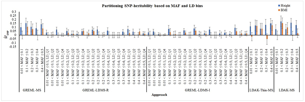
Partitioning the SNP-heritability using MAF and LD bins. For GREML-MS, LDAK-Thin-MS and LDAK-MS, MAF bins were created as 0.01 < MAF ≤ 0.1, 0.1 < MAF ≤ 0.2, 0.2 < MAF ≤ 0.3, 0.3 < MAF ≤ 0.4 and 0.4 < MAF ≤ 0.5. For GREML-LDMS, each MAF bin was further divided into quartiles of average regional LD score or SNP LD score.

Table 3: Comparison of SNP-heritability (${\widehat{\mathrm{h}}}_{\mathrm{S}\mathrm{N}\mathrm{P}}^2$) of height and BMI attributable to various MAF and LD bins utilizing stratified-GREML and stratified-LDAK analyses:

MS, LDMS-R, LDMS-I represent MAF stratified, Regional LD scores and MAF stratified, Individual SNP LD score and MAF stratified, respectively; LD_Q1-4 represent quartiles one to four based on regional or SNP LD scores. P-values were calculated using one sided z test.

Approach	Bins	Height			BMI
		${\widehat{\mathbf{h}}}_{\mathbf{S}\mathbf{N}\mathbf{P}}^2$	S.E.	P-Value	${\widehat{\mathbf{h}}}_{\mathbf{S}\mathbf{N}\mathbf{P}}^2$	S.E.	P-Value
GREML-MS	0.01 < MAF ≤ 0.1	0.0999	0.0531	2.99E-02	0.0021	0.0513	4.84E-01
	0.1 < MAF ≤ 0.2	0.1531	0.0656	9.81E-03	0.1076	0.0663	5.24E-02
	0.2 < MAF ≤ 0.3	0.1075	0.0655	5.03E-02	0.0766	0.0664	1.25E-01
	0.3 < MAF ≤ 0.4	0.0878	0.0665	9.33E-02	0.0000	0.0646	5.00E-01
	0.4 < MAF ≤ 0.5	0.1383	0.0594	9.94E-03	0.0851	0.0601	7.85E-02
GREML-LDMS-R	0.01 < MAF ≤ 0.1; LD_Q1	0.0324	0.0312	1.50E-01	0.0000	0.0322	5.00E-01
	0.01 < MAF ≤ 0.1; LD_Q2	0.0000	0.0305	5.00E-01	0.0079	0.0312	4.00E-01
	0.01 < MAF ≤ 0.1; LD_Q3	0.0713	0.0299	8.45E-03	0.0000	0.0291	5.00E-01
	0.01 < MAF ≤ 0.1; LD_Q4	0.0053	0.0211	4.01E-01	0.0014	0.0214	4.74E-01
	0.1 < MAF ≤ 0.2; LD_Q1	0.0502	0.0395	1.02E-01	0.0279	0.0410	2.48E-01
	0.1 < MAF ≤ 0.2; LD_Q2	0.0143	0.0380	3.54E-01	0.0143	0.0378	3.53E-01
	0.1 < MAF ≤ 0.2; LD_Q3	0.0166	0.0344	3.15E-01	0.0000	0.0354	5.00E-01
	0.1 < MAF ≤ 0.2; LD_Q4	0.0473	0.0272	4.11E-02	0.0530	0.0283	3.07E-02
	0.2 < MAF ≤ 0.3; LD_Q1	0.0000	0.0379	5.00E-01	0.0250	0.0398	2.65E-01
	0.2 < MAF ≤ 0.3; LD_Q2	0.0668	0.0373	3.67E-02	0.0507	0.0380	9.10E-02
	0.2 < MAF ≤ 0.3; LD_Q3	0.0710	0.0362	2.50E-02	0.0050	0.0354	4.44E-01
	0.2 < MAF ≤ 0.3; LD_Q4	0.0000	0.0276	5.00E-01	0.0081	0.0282	3.87E-01
	0.3 < MAF ≤ 0.4; LD_Q1	0.0556	0.0383	7.37E-02	0.0010	0.0392	4.89E-01
	0.3 < MAF ≤ 0.4; LD_Q2	0.0001	0.0360	4.99E-01	0.0000	0.0361	5.00E-01
	0.3 < MAF ≤ 0.4; LD_Q3	0.0000	0.0345	5.00E-01	0.0000	0.0345	5.00E-01
	0.3 < MAF ≤ 0.4; LD_Q4	0.0425	0.0290	7.12E-02	0.0000	0.0276	5.00E-01
	0.4 < MAF ≤ 0.5; LD_Q1	0.0766	0.0358	1.62E-02	0.0254	0.0360	2.40E-01
	0.4 < MAF ≤ 0.5; LD_Q2	0.0436	0.0336	9.72E-02	0.0000	0.0334	5.00E-01
	0.4 < MAF ≤ 0.5; LD_Q3	0.0035	0.0307	4.54E-01	0.0457	0.0319	7.56E-02
	0.4 < MAF ≤ 0.5; LD_Q4	0.0201	0.0246	2.06E-01	0.0157	0.0257	2.72E-01
GREML-LDMS-I	0.01 < MAF ≤ 0.1; LD_Q1	0.0340	0.0462	2.31E-01	0.0000	0.0486	5.00E-01
	0.01 < MAF ≤ 0.1; LD_Q2	0.0462	0.0284	5.18E-02	0.0000	0.0283	5.00E-01
	0.01 < MAF ≤ 0.1; LD_Q3	0.0107	0.0190	2.87E-01	0.0064	0.0192	3.70E-01
	0.01 < MAF ≤ 0.1; LD_Q4	0.0000	0.0099	5.00E-01	0.0050	0.0109	3.22E-01
	0.1 < MAF ≤ 0.2; LD_Q1	0.0786	0.0452	4.11E-02	0.0364	0.0460	2.14E-01
	0.1 < MAF ≤ 0.2; LD_Q2	0.0071	0.0404	4.30E-01	0.0108	0.0410	3.96E-01
	0.1 < MAF ≤ 0.2; LD_Q3	0.0000	0.0334	5.00E-01	0.0019	0.0336	4.77E-01
	0.1 < MAF ≤ 0.2; LD_Q4	0.0599	0.0230	4.58E-03	0.0309	0.0227	8.70E-02
	0.2 < MAF ≤ 0.3; LD_Q1	0.0000	0.0374	5.00E-01	0.0004	0.0381	4.96E-01
	0.2 < MAF ≤ 0.3; LD_Q2	0.0854	0.0405	1.76E-02	0.0562	0.0404	8.21E-02
	0.2 < MAF ≤ 0.3; LD_Q3	0.0137	0.0358	3.51E-01	0.0002	0.0380	4.98E-01
	0.2 < MAF ≤ 0.3; LD_Q4	0.0249	0.0282	1.89E-01	0.0156	0.0283	2.91E-01
	0.3 < MAF ≤ 0.4; LD_Q1	0.0700	0.0334	1.82E-02	0.0000	0.0347	5.00E-01
	0.3 < MAF ≤ 0.4; LD_Q2	0.0000	0.0378	5.00E-01	0.0000	0.0391	5.00E-01
	0.3 < MAF ≤ 0.4; LD_Q3	0.0219	0.0372	2.77E-01	0.0000	0.0379	5.00E-01
	0.3 < MAF ≤ 0.4; LD_Q4	0.0295	0.0309	1.70E-01	0.0000	0.0300	5.00E-01
	0.4 < MAF ≤ 0.5; LD_Q1	0.0141	0.0314	3.27E-01	0.0000	0.0316	5.00E-01
	0.4 < MAF ≤ 0.5; LD_Q2	0.0938	0.0362	4.79E-03	0.0483	0.0372	9.68E-02
	0.4 < MAF ≤ 0.5; LD_Q3	0.0060	0.0346	4.31E-01	0.0211	0.0358	2.78E-01
	0.4 < MAF ≤ 0.5; LD_Q4	0.0195	0.0278	2.41E-01	0.0196	0.0292	2.51E-01
LDAK-Thin-MS	0.01 < MAF ≤ 0.1	0.1112	0.0554	2.24E-02	-0.0201	0.0539	3.54E-01
	0.1 < MAF ≤ 0.2	0.1243	0.0695	3.68E-02	0.1175	0.0704	4.76E-02
	0.2 < MAF ≤ 0.3	0.0820	0.0699	1.20E-01	0.0822	0.0696	1.19E-01
	0.3 < MAF ≤ 0.4	0.1306	0.0703	3.17E-02	-0.0518	0.0692	2.27E-01
	0.4 < MAF ≤ 0.5	0.1495	0.0630	8.82E-03	0.1250	0.0639	2.53E-02
LDAK-MS	0.01 < MAF ≤ 0.1	0.0767	0.0569	8.88E-02	-0.0034	0.0569	4.76E-01
	0.1 < MAF ≤ 0.2	0.1769	0.0678	4.52E-03	0.1525	0.0691	1.37E-02
	0.2 < MAF ≤ 0.3	0.0763	0.0623	1.10E-01	0.0970	0.0626	6.05E-02
	0.3 < MAF ≤ 0.4	0.1576	0.0585	3.52E-03	-0.0099	0.0591	4.33E-01
	0.4 < MAF ≤ 0.5	0.1298	0.0570	1.14E-02	0.0237	0.0567	3.38E-01

Conclusion and Future direction

Heritability has been widely used to improve the quality of crops and farm animals, to understand the genetic basis of complex human traits and related diseases, and to estimate the response of evolutionary forces such as selection in a population. However, the utility of heritability has been limited to a certain extent, mainly due to lack of appropriate data types and heritability models. Over the past decade, several approaches fitting a variety of analytical models have been developed to estimate SNP-heritability in unrelated individuals. In the current review, we provide an overview of these approaches along with step-by-step protocol to run widely used approaches for SNP-heritability estimation.

Despite advances in heritability models and availability of genome-wide SNPs information in large datasets, estimates of ${\mathrm{h}}_{\mathrm{S}\mathrm{N}\mathrm{P}}^2$ are one third to two third of the heritability estimated through family-based approaches. With the availability of whole genome sequence (WGS) information in large data sets, population-based approaches can be used to estimate the variance attributable to all variants (including rare variants) that should bring estimates from the two approaches closer. Such datasets also demand development of integrative models that can fit other types of genetic variations such as structural and copy number variants into the LMM. Inclusion of rare variants and other types of variants should not only resolve the problem of incomplete tagging of causal variants but also fill the gap of missing heritability. However, selection of appropriate heritability models for different data types and their precision still present an ongoing debate(Speed et al., 2020; Zhu & Zhou, 2020). Therefore, a consensus needs to be reached regarding heritability models for different data types. Previously, some efforts were made to estimate SNP-heritability utilizing identity-by-descent information inferred from genome-wide data(Browning & Browning, 2013; Evans, Tahmasbi, Jones, et al., 2018). In near future, we can expect new and better approaches that can estimate unbiased ${\mathrm{h}}_{\mathrm{S}\mathrm{N}\mathrm{P}}^2$ from identity-by-descent information inferred from WGS data. Likewise, methods using pedigree data to estimate narrow-sense heritability should account for shared environmental effects and assortative mating. Moreover, new methods to estimate heritability free of assumptions about the relationship between effect size and minor allele frequency are also required in near future.

Data Availability Statement

Individual-level genetic data that support the protocol (The Northern Finland Birth Cohort) are available in dbGaP for general research use (https://www.ncbi.nlm.nih.gov/projects/gap/cgi-bin/study.cgi?study_id=phs000276.v2.p1). Likewise, summary results are openly available in GIANT consortium datafiles (https://portals.broadinstitute.org/collaboration/giant/index.php/GIANT_consortium_data_files)

Literature Cited

- Allison DB, Kaprio J, Korkeila M, Koskenvuo M, Neale MC, & Hayakawa K (1996). The heritability of body mass index among an international sample of monozygotic twins reared apart. Int J Obes Relat Metab Disord, 20(6), 501–506. Retrieved from https://www.ncbi.nlm.nih.gov/pubmed/8782724 [PubMed] [Google Scholar]
- Alvarez D. V.-M. a. J. C. (2017). Genetic Improvement of Oilseed Crops Using Modern Biotechnology. In Jimenez-Lopez JC (Ed.), Advances in Seed Biology. [Google Scholar]
- Bateson W (1922). Genetical Analysis and the Theory of Natural Selection. Science, 55(1423), 373. doi: 10.1126/science.55.1423.373 [DOI] [PubMed] [Google Scholar]
- Bernardo R (2020). Reinventing quantitative genetics for plant breeding: something old, something new, something borrowed, something BLUE. Heredity (Edinb), 125(6), 375–385. doi: 10.1038/s41437-020-0312-1 [DOI] [PMC free article] [PubMed] [Google Scholar]
- Berry DP, Buckley F, Dillon P, Evans RD, Rath M, & Veerkamp RF (2003). Genetic parameters for body condition score, body weight, milk yield, and fertility estimated using random regression models. J Dairy Sci, 86(11), 3704–3717. doi: 10.3168/jds.S0022-0302(03)73976-9 [DOI] [PubMed] [Google Scholar]
- Berry DP, Wall E, & Pryce JE (2014). Genetics and genomics of reproductive performance in dairy and beef cattle. Animal, 8 Suppl 1, 105–121. doi: 10.1017/S1751731114000743 [DOI] [PubMed] [Google Scholar]
- Boomsma D, Busjahn A, & Peltonen L (2002). Classical twin studies and beyond. Nat Rev Genet, 3(11), 872–882. doi: 10.1038/nrg932 [DOI] [PubMed] [Google Scholar]
- Brookfield JF (2013). Quantitative genetics: heritability is not always missing. Curr Biol, 23(7), R276–278. doi: 10.1016/j.cub.2013.02.040 [DOI] [PubMed] [Google Scholar]
- Browning SR, & Browning BL (2012). Identity by descent between distant relatives: detection and applications. Annu Rev Genet, 46, 617–633. doi: 10.1146/annurev-genet-110711-155534 [DOI] [PubMed] [Google Scholar]
- Browning SR, & Browning BL (2013). Identity-by-descent-based heritability analysis in the Northern Finland Birth Cohort. Hum Genet, 132(2), 129–138. doi: 10.1007/s00439-012-1230-y [DOI] [PMC free article] [PubMed] [Google Scholar]
- Bulik-Sullivan B, Finucane HK, Anttila V, Gusev A, Day FR, Loh PR, … Neale BM. (2015). An atlas of genetic correlations across human diseases and traits. Nat Genet, 47(11), 1236–1241. doi: 10.1038/ng.3406 [DOI] [PMC free article] [PubMed] [Google Scholar]
- Bulik-Sullivan BK, Loh PR, Finucane HK, Ripke S, Yang J, Schizophrenia Working Group of the Psychiatric Genomics, C., … Neale BM. (2015). LD Score regression distinguishes confounding from polygenicity in genome-wide association studies. Nat Genet, 47(3), 291–295. doi: 10.1038/ng.3211 [DOI] [PMC free article] [PubMed] [Google Scholar]
- Buniello A, MacArthur JAL, Cerezo M, Harris LW, Hayhurst J, Malangone C, … Parkinson H. (2019). The NHGRI-EBI GWAS Catalog of published genome-wide association studies, targeted arrays and summary statistics 2019. Nucleic Acids Res, 47(D1), D1005–D1012. doi: 10.1093/nar/gky1120 [DOI] [PMC free article] [PubMed] [Google Scholar]
- Cassell BG (2009). Using heritability for genetic improvement.
- Chang CC, Chow CC, Tellier LC, Vattikuti S, Purcell SM, & Lee JJ (2015). Second-generation PLINK: rising to the challenge of larger and richer datasets. Gigascience, 4, 7. doi: 10.1186/s13742-015-0047-8 [DOI] [PMC free article] [PubMed] [Google Scholar]
- Dempster ER, & Lerner IM (1950). Heritability of Threshold Characters. Genetics, 35(2), 212–236. doi: 10.1093/genetics/35.2.212 [DOI] [PMC free article] [PubMed] [Google Scholar]
- Eaves LJ, Last KA, Young PA, & Martin NG (1978). Model-fitting approaches to the analysis of human behaviour. Heredity (Edinb), 41(3), 249–320. Retrieved from https://www.ncbi.nlm.nih.gov/pubmed/370072 [DOI] [PubMed] [Google Scholar]
- Eichler EE, Flint J, Gibson G, Kong A, Leal SM, Moore JH, & Nadeau JH (2010). Missing heritability and strategies for finding the underlying causes of complex disease. Nat Rev Genet, 11(6), 446–450. doi: 10.1038/nrg2809 [DOI] [PMC free article] [PubMed] [Google Scholar]
- Evans LM, Tahmasbi R, Jones M, Vrieze SI, Abecasis GR, Das S, … Haplotype Reference, C. (2018). Narrow-sense heritability estimation of complex traits using identity-by-descent information. Heredity (Edinb), 121(6), 616–630. doi: 10.1038/s41437-018-0067-0 [DOI] [PMC free article] [PubMed] [Google Scholar]
- Evans LM, Tahmasbi R, Vrieze SI, Abecasis GR, Das S, Gazal S, … Keller MC. (2018). Comparison of methods that use whole genome data to estimate the heritability and genetic architecture of complex traits. Nat Genet, 50(5), 737–745. doi: 10.1038/s41588-018-0108-x [DOI] [PMC free article] [PubMed] [Google Scholar]
- Falconer DS (1960). Introduction to Quantitative Genetics (1 ed.). Edinburgh/London: Oliver & Boyd. [Google Scholar]
- Falconer DS (1965). Inheritance of liabillity to certain diseases, estimated from the incidence among relatives. Annals of Human Genetics, 29(1), 51–76. [Google Scholar]
- Finucane HK, Bulik-Sullivan B, Gusev A, Trynka G, Reshef Y, Loh PR, … Price AL. (2015). Partitioning heritability by functional annotation using genome-wide association summary statistics. Nat Genet, 47(11), 1228–1235. doi: 10.1038/ng.3404 [DOI] [PMC free article] [PubMed] [Google Scholar]
- Fisher RA (1918). The Correlation between Relatives on the Supposition of Mendelian Inheritance. Transactions of the Royal Society of Edinburgh, 52, 35. [Google Scholar]
- Fisher RA (1930). The genetical theory of natural selection. Oxford, England: Clarendon Press. [Google Scholar]
- Friedman NP, Banich MT, & Keller MC (2021). Twin studies to GWAS: there and back again. Trends Cogn Sci, 25(10), 855–869. doi: 10.1016/j.tics.2021.06.007 [DOI] [PMC free article] [PubMed] [Google Scholar]
- Genin E (2020). Missing heritability of complex diseases: case solved? Hum Genet, 139(1), 103–113. doi: 10.1007/s00439-019-02034-4 [DOI] [PubMed] [Google Scholar]
- Genomes Project C, Abecasis GR, Altshuler D, Auton A, Brooks LD, Durbin RM, … McVean GA. (2010). A map of human genome variation from population-scale sequencing. Nature, 467(7319), 1061–1073. doi: 10.1038/nature09534 [DOI] [PMC free article] [PubMed] [Google Scholar]
- Genomes Project C, Abecasis GR, Auton A, Brooks LD, DePristo MA, Durbin RM, … McVean GA. (2012). An integrated map of genetic variation from 1,092 human genomes. Nature, 491(7422), 56–65. doi: 10.1038/nature11632 [DOI] [PMC free article] [PubMed] [Google Scholar]
- Genomes Project C, Auton A, Brooks LD, Durbin RM, Garrison EP, Kang HM, … Abecasis GR. (2015). A global reference for human genetic variation. Nature, 526(7571), 68–74. doi: 10.1038/nature15393 [DOI] [PMC free article] [PubMed] [Google Scholar]
- Gibson G (2012). Rare and common variants: twenty arguments. Nat Rev Genet, 13(2), 135–145. doi: 10.1038/nrg3118 [DOI] [PMC free article] [PubMed] [Google Scholar]
- Golan D, Lander ES, & Rosset S (2014). Measuring missing heritability: inferring the contribution of common variants. Proc Natl Acad Sci U S A, 111(49), E5272–5281. doi: 10.1073/pnas.1419064111 [DOI] [PMC free article] [PubMed] [Google Scholar]
- Grant PR, & Grant BR (1995). Predicting Microevolutionary Responses to Directional Selection on Heritable Variation. Evolution, 49(2), 241–251. doi: 10.1111/j.1558-5646.1995.tb02236.x [DOI] [PubMed] [Google Scholar]
- Hadfield JD (2008). Estimating evolutionary parameters when viability selection is operating. Proc Biol Sci, 275(1635), 723–734. doi: 10.1098/rspb.2007.1013 [DOI] [PMC free article] [PubMed] [Google Scholar]
- Hall JB, & Bush WS (2016). Analysis of Heritability Using Genome-Wide Data. Curr Protoc Hum Genet, 91, 1 30 31–31 30 10. doi: 10.1002/cphg.25 [DOI] [PMC free article] [PubMed] [Google Scholar]
- Haseman JK, & Elston RC (1972). The investigation of linkage between a quantitative trait and a marker locus. Behav Genet, 2(1), 3–19. doi: 10.1007/BF01066731 [DOI] [PubMed] [Google Scholar]
- Hou K, Burch KS, Majumdar A, Shi H, Mancuso N, Wu Y, … Pasaniuc B. (2019). Accurate estimation of SNP-heritability from biobank-scale data irrespective of genetic architecture. Nat Genet, 51(8), 1244–1251. doi: 10.1038/s41588-019-0465-0 [DOI] [PMC free article] [PubMed] [Google Scholar]
- International HapMap C (2005). A haplotype map of the human genome. Nature, 437(7063), 1299–1320. doi: 10.1038/nature04226 [DOI] [PMC free article] [PubMed] [Google Scholar]
- Kelly JK (2011). The breeder’s equation. Nature Education Knowledge. 4(5):5. Retrieved from https://www.nature.com/scitable/knowledge/library/the-breeder-s-equation-24204828/ [Google Scholar]
- Kingsolver JG, Hoekstra HE, Hoekstra JM, Berrigan D, Vignieri SN, Hill CE, … Beerli P. (2001). The strength of phenotypic selection in natural populations. Am Nat, 157(3), 245–261. doi: 10.1086/319193 [DOI] [PubMed] [Google Scholar]
- Lande R, & Arnold SJ (1983). The Measurement of Selection on Correlated Characters. Evolution, 37(6), 1210–1226. doi: 10.1111/j.1558-5646.1983.tb00236.x [DOI] [PubMed] [Google Scholar]
- Lee SH, Goddard ME, Visscher PM, & van der Werf JH (2010). Using the realized relationship matrix to disentangle confounding factors for the estimation of genetic variance components of complex traits. Genet Sel Evol, 42(1), 22. doi: 10.1186/1297-9686-42-22 [DOI] [PMC free article] [PubMed] [Google Scholar]
- Lee SH, & van der Werf JH (2006). An efficient variance component approach implementing an average information REML suitable for combined LD and linkage mapping with a general complex pedigree. Genet Sel Evol, 38(1), 25–43. doi: 10.1051/gse:2005025 [DOI] [PMC free article] [PubMed] [Google Scholar]
- Lee SH, Wray NR, Goddard ME, & Visscher PM (2011). Estimating missing heritability for disease from genome-wide association studies. Am J Hum Genet, 88(3), 294–305. doi: 10.1016/j.ajhg.2011.02.002 [DOI] [PMC free article] [PubMed] [Google Scholar]
- Lunde A, Melve KK, Gjessing HK, Skjaerven R, & Irgens LM (2007). Genetic and environmental influences on birth weight, birth length, head circumference, and gestational age by use of population-based parent-offspring data. Am J Epidemiol, 165(7), 734–741. doi: 10.1093/aje/kwk107 [DOI] [PubMed] [Google Scholar]
- Manjula P, Park HB, Seo D, Choi N, Jin S, Ahn SJ, … Lee JH. (2018). Estimation of heritability and genetic correlation of body weight gain and growth curve parameters in Korean native chicken. Asian-Australas J Anim Sci, 31(1), 26–31. doi: 10.5713/ajas.17.0179 [DOI] [PMC free article] [PubMed] [Google Scholar]
- Manolio TA, Collins FS, Cox NJ, Goldstein DB, Hindorff LA, Hunter DJ, … Visscher PM. (2009). Finding the missing heritability of complex diseases. Nature, 461(7265), 747–753. doi: 10.1038/nature08494 [DOI] [PMC free article] [PubMed] [Google Scholar]
- Maroilley T, & Tarailo-Graovac M (2019). Uncovering Missing Heritability in Rare Diseases. Genes (Basel), 10(4). doi: 10.3390/genes10040275 [DOI] [PMC free article] [PubMed] [Google Scholar]
- Mayhew AJ, & Meyre D (2017). Assessing the Heritability of Complex Traits in Humans: Methodological Challenges and Opportunities. Curr Genomics, 18(4), 332–340. doi: 10.2174/1389202918666170307161450 [DOI] [PMC free article] [PubMed] [Google Scholar]
- Medicine I. o. (2006). Genetics and Health. In Hernandez LM & Blazer DG (Eds.), Genes, Behavior, and the Social Environment: Moving Beyond the Nature/Nurture Debate (pp. 384). Washington, DC: The National Academies Press. [PubMed] [Google Scholar]
- Miglior F, Fleming A, Malchiodi F, Brito LF, Martin P, & Baes CF (2017). A 100-Year Review: Identification and genetic selection of economically important traits in dairy cattle. J Dairy Sci, 100(12), 10251–10271. doi: 10.3168/jds.2017-12968 [DOI] [PubMed] [Google Scholar]
- Mousseau TA, & Roff DA (1987). Natural selection and the heritability of fitness components. Heredity (Edinb), 59 ( Pt 2), 181–197. doi: 10.1038/hdy.1987.113 [DOI] [PubMed] [Google Scholar]
- Nance WE, Kramer AA, Corey LA, Winter PM, & Eaves LJ (1983). A causal analysis of birth weight in the offspring of monozygotic twins. Am J Hum Genet, 35(6), 1211–1223. Retrieved from https://www.ncbi.nlm.nih.gov/pubmed/6685976 [PMC free article] [PubMed] [Google Scholar]
- Ni G, Moser G, Schizophrenia Working Group of the Psychiatric Genomics, C., Wray NR, & Lee SH. (2018). Estimation of Genetic Correlation via Linkage Disequilibrium Score Regression and Genomic Restricted Maximum Likelihood. Am J Hum Genet, 102(6), 1185–1194. doi: 10.1016/j.ajhg.2018.03.021 [DOI] [PMC free article] [PubMed] [Google Scholar]
- Palmquist DL, & Jenkins TC (2017). A 100-Year Review: Fat feeding of dairy cows. J Dairy Sci, 100(12), 10061–10077. doi: 10.3168/jds.2017-12924 [DOI] [PubMed] [Google Scholar]
- Pasaniuc B, & Price AL (2017). Dissecting the genetics of complex traits using summary association statistics. Nat Rev Genet, 18(2), 117–127. doi: 10.1038/nrg.2016.142 [DOI] [PMC free article] [PubMed] [Google Scholar]
- Powell JE, Visscher PM, & Goddard ME (2010). Reconciling the analysis of IBD and IBS in complex trait studies. Nat Rev Genet, 11(11), 800–805. doi: 10.1038/nrg2865 [DOI] [PubMed] [Google Scholar]
- Purcell S, Neale B, Todd-Brown K, Thomas L, Ferreira MA, Bender D, … Sham PC. (2007). PLINK: a tool set for whole-genome association and population-based linkage analyses. Am J Hum Genet, 81(3), 559–575. doi: 10.1086/519795 [DOI] [PMC free article] [PubMed] [Google Scholar]
- Ritland K (1996). A Marker-Based Method for Inferences About Quantitative Inheritance in Natural Populations. Evolution, 50(3), 1062–1073. doi: 10.1111/j.1558-5646.1996.tb02347.x [DOI] [PubMed] [Google Scholar]
- Ritland K (2000). Marker-inferred relatedness as a tool for detecting heritability in nature. Mol Ecol, 9(9), 1195–1204. doi: 10.1046/j.1365-294x.2000.00971.x [DOI] [PubMed] [Google Scholar]
- Sabatti C, Service SK, Hartikainen AL, Pouta A, Ripatti S, Brodsky J, … Peltonen L. (2009). Genome-wide association analysis of metabolic traits in a birth cohort from a founder population. Nat Genet, 41(1), 35–46. doi: 10.1038/ng.271 [DOI] [PMC free article] [PubMed] [Google Scholar]
- Sham PC, & Purcell S (2001). Equivalence between Haseman-Elston and variance-components linkage analyses for sib pairs. Am J Hum Genet, 68(6), 1527–1532. doi: 10.1086/320593 [DOI] [PMC free article] [PubMed] [Google Scholar]
- Silventoinen K, Sammalisto S, Perola M, Boomsma DI, Cornes BK, Davis C, … Kaprio J. (2003). Heritability of adult body height: a comparative study of twin cohorts in eight countries. Twin Res, 6(5), 399–408. doi: 10.1375/136905203770326402 [DOI] [PubMed] [Google Scholar]
- Speed D, & Balding DJ (2015). Relatedness in the post-genomic era: is it still useful? Nat Rev Genet, 16(1), 33–44. doi: 10.1038/nrg3821 [DOI] [PubMed] [Google Scholar]
- Speed D, & Balding DJ (2019). SumHer better estimates the SNP heritability of complex traits from summary statistics. Nat Genet, 51(2), 277–284. doi: 10.1038/s41588-018-0279-5 [DOI] [PMC free article] [PubMed] [Google Scholar]
- Speed D, Cai N, Consortium U, Johnson MR, Nejentsev S, & Balding DJ (2017). Reevaluation of SNP heritability in complex human traits. Nat Genet, 49(7), 986–992. doi: 10.1038/ng.3865 [DOI] [PMC free article] [PubMed] [Google Scholar]
- Speed D, Hemani G, Johnson MR, & Balding DJ (2012). Improved heritability estimation from genome-wide SNPs. Am J Hum Genet, 91(6), 1011–1021. doi: 10.1016/j.ajhg.2012.10.010 [DOI] [PMC free article] [PubMed] [Google Scholar]
- Speed D, Holmes J, & Balding DJ (2020). Evaluating and improving heritability models using summary statistics. Nat Genet, 52(4), 458–462. doi: 10.1038/s41588-020-0600-y [DOI] [PubMed] [Google Scholar]
- Stunkard AJ, Harris JR, Pedersen NL, & McClearn GE (1990). The body-mass index of twins who have been reared apart. N Engl J Med, 322(21), 1483–1487. doi: 10.1056/NEJM199005243222102 [DOI] [PubMed] [Google Scholar]
- Tang M, Wang T, & Zhang X (2022). A review of SNP heritability estimation methods. Brief Bioinform, 23(3). doi: 10.1093/bib/bbac067 [DOI] [PubMed] [Google Scholar]
- Team R (2019). RStudio: Integrated Development for R. Boston, MA: RStudio, Inc. Retrieved from http://www.rstudio.com/ [Google Scholar]
- Team, R. C. (2020). R: A Language and Environment for Statistical Computing. Vienna, Austria: R Foundation for Statistical Computing. Retrieved from https://www.R-project.org/ [Google Scholar]
- Tenesa A, & Haley CS (2013). The heritability of human disease: estimation, uses and abuses. Nat Rev Genet, 14(2), 139–149. doi: 10.1038/nrg3377 [DOI] [PubMed] [Google Scholar]
- Thomas SC (2005). The estimation of genetic relationships using molecular markers and their efficiency in estimating heritability in natural populations. Philos Trans R Soc Lond B Biol Sci, 360(1459), 1457–1467. doi: 10.1098/rstb.2005.1675 [DOI] [PMC free article] [PubMed] [Google Scholar]
- Thompson H. D. P. a. R. (1971). Recovery of Inter-Block Information when Block Sizes are Unequal. Biometrika, 58(3), 545–554. [Google Scholar]
- Truong VQ, Woerner JA, Cherlin TA, Bradford Y, Lucas AM, Okeh CC, … Verma SS. (2022). Quality Control Procedures for Genome-Wide Association Studies. Curr Protoc, 2(11), e603. doi: 10.1002/cpz1.603 [DOI] [PubMed] [Google Scholar]
- Turner S, Armstrong LL, Bradford Y, Carlson CS, Crawford DC, Crenshaw AT, … Ritchie MD. (2011). Quality control procedures for genome-wide association studies. Curr Protoc Hum Genet, Chapter 1, Unit 1 19. doi: 10.1002/0471142905.hg0119s68 [DOI] [PMC free article] [PubMed] [Google Scholar]
- Uricchio LH (2020). Evolutionary perspectives on polygenic selection, missing heritability, and GWAS. Hum Genet, 139(1), 5–21. doi: 10.1007/s00439-019-02040-6 [DOI] [PMC free article] [PubMed] [Google Scholar]
- Utrera AR, & Van Vleck LD (2004). Heritability estimates for carcass traits of cattle: a review. Genet Mol Res, 3(3), 380–394. Retrieved from https://www.ncbi.nlm.nih.gov/pubmed/15614729 [PubMed] [Google Scholar]
- VanRaden PM (2008). Efficient methods to compute genomic predictions. J Dairy Sci, 91(11), 4414–4423. doi: 10.3168/jds.2007-0980 [DOI] [PubMed] [Google Scholar]
- Velasco L, & Fernández-martínez JM (2002). Breeding Oilseed Crops for Improved Oil Quality. Journal of Crop Production, 5(1–2), 309–344. doi: 10.1300/J144v05n01_13 [DOI] [Google Scholar]
- Vinkhuyzen AA, Wray NR, Yang J, Goddard ME, & Visscher PM (2013). Estimation and partition of heritability in human populations using whole-genome analysis methods. Annu Rev Genet, 47, 75–95. doi: 10.1146/annurev-genet-111212-133258 [DOI] [PMC free article] [PubMed] [Google Scholar]
- Visscher PM, & Goddard ME (2019). From R.A. Fisher’s 1918 Paper to GWAS a Century Later. Genetics, 211(4), 1125–1130. doi: 10.1534/genetics.118.301594 [DOI] [PMC free article] [PubMed] [Google Scholar]
- Visscher PM, Hill WG, & Wray NR (2008). Heritability in the genomics era--concepts and misconceptions. Nat Rev Genet, 9(4), 255–266. doi: 10.1038/nrg2322 [DOI] [PubMed] [Google Scholar]
- Visscher PM, Macgregor S, Benyamin B, Zhu G, Gordon S, Medland S, … Martin NG. (2007). Genome partitioning of genetic variation for height from 11,214 sibling pairs. Am J Hum Genet, 81(5), 1104–1110. doi: 10.1086/522934 [DOI] [PMC free article] [PubMed] [Google Scholar]
- Visscher PM, McEvoy B, & Yang J (2010). From Galton to GWAS: quantitative genetics of human height. Genet Res (Camb), 92(5–6), 371–379. doi: 10.1017/S0016672310000571 [DOI] [PubMed] [Google Scholar]
- Visscher PM, Medland SE, Ferreira MA, Morley KI, Zhu G, Cornes BK, … Martin NG. (2006). Assumption-free estimation of heritability from genome-wide identity-by-descent sharing between full siblings. PLoS Genet, 2(3), e41. doi: 10.1371/journal.pgen.0020041 [DOI] [PMC free article] [PubMed] [Google Scholar]
- Walsh M. L. a. B. (1998). Genetics and Analysis of Quantitative Traits. Sunderland, MA: Sinauer Associates, Inc. [Google Scholar]
- Weale ME (2010). Quality control for genome-wide association studies. Methods Mol Biol, 628, 341–372. doi: 10.1007/978-1-60327-367-1_19 [DOI] [PubMed] [Google Scholar]
- Weir BS, Anderson AD, & Hepler AB (2006). Genetic relatedness analysis: modern data and new challenges. Nat Rev Genet, 7(10), 771–780. doi: 10.1038/nrg1960 [DOI] [PubMed] [Google Scholar]
- Wood JL, Yates MC, & Fraser DJ (2016). Are heritability and selection related to population size in nature? Meta-analysis and conservation implications. Evol Appl, 9(5), 640–657. doi: 10.1111/eva.12375 [DOI] [PMC free article] [PubMed] [Google Scholar]
- Wray NR, Goddard ME, & Visscher PM (2007). Prediction of individual genetic risk to disease from genome-wide association studies. Genome Res, 17(10), 1520–1528. doi: 10.1101/gr.6665407 [DOI] [PMC free article] [PubMed] [Google Scholar]
- Wray NR, Yang J, Hayes BJ, Price AL, Goddard ME, & Visscher PM (2013). Pitfalls of predicting complex traits from SNPs. Nat Rev Genet, 14(7), 507–515. doi: 10.1038/nrg3457 [DOI] [PMC free article] [PubMed] [Google Scholar]
- Wright S (1921). Systems of Mating. I. the Biometric Relations between Parent and Offspring. Genetics, 6(2), 111–123. doi: 10.1093/genetics/6.2.111 [DOI] [PMC free article] [PubMed] [Google Scholar]
- Yang J, Bakshi A, Zhu Z, Hemani G, Vinkhuyzen AA, Lee SH, … Visscher PM. (2015). Genetic variance estimation with imputed variants finds negligible missing heritability for human height and body mass index. Nat Genet, 47(10), 1114–1120. doi: 10.1038/ng.3390 [DOI] [PMC free article] [PubMed] [Google Scholar]
- Yang J, Benyamin B, McEvoy BP, Gordon S, Henders AK, Nyholt DR, … Visscher PM. (2010). Common SNPs explain a large proportion of the heritability for human height. Nat Genet, 42(7), 565–569. doi: 10.1038/ng.608 [DOI] [PMC free article] [PubMed] [Google Scholar]
- Yang J, Lee SH, Goddard ME, & Visscher PM (2011). GCTA: a tool for genome-wide complex trait analysis. Am J Hum Genet, 88(1), 76–82. doi: 10.1016/j.ajhg.2010.11.011 [DOI] [PMC free article] [PubMed] [Google Scholar]
- Yang J, Lee SH, Goddard ME, & Visscher PM (2013). Genome-wide complex trait analysis (GCTA): methods, data analyses, and interpretations. Methods Mol Biol, 1019, 215–236. doi: 10.1007/978-1-62703-447-0_9 [DOI] [PubMed] [Google Scholar]
- Yang J, Manolio TA, Pasquale LR, Boerwinkle E, Caporaso N, Cunningham JM, … Visscher PM. (2011). Genome partitioning of genetic variation for complex traits using common SNPs. Nat Genet, 43(6), 519–525. doi: 10.1038/ng.823 [DOI] [PMC free article] [PubMed] [Google Scholar]
- Yang J, Zaitlen NA, Goddard ME, Visscher PM, & Price AL (2014). Advantages and pitfalls in the application of mixed-model association methods. Nat Genet, 46(2), 100–106. doi: 10.1038/ng.2876 [DOI] [PMC free article] [PubMed] [Google Scholar]
- Yang J, Zeng J, Goddard ME, Wray NR, & Visscher PM (2017). Concepts, estimation and interpretation of SNP-based heritability. Nat Genet, 49(9), 1304–1310. doi: 10.1038/ng.3941 [DOI] [PubMed] [Google Scholar]
- Yengo L, Sidorenko J, Kemper KE, Zheng Z, Wood AR, Weedon MN, … Consortium, G. (2018). Meta-analysis of genome-wide association studies for height and body mass index in approximately 700000 individuals of European ancestry. Hum Mol Genet, 27(20), 3641–3649. doi: 10.1093/hmg/ddy271 [DOI] [PMC free article] [PubMed] [Google Scholar]
- Zaitlen N, & Kraft P (2012). Heritability in the genome-wide association era. Hum Genet, 131(10), 1655–1664. doi: 10.1007/s00439-012-1199-6 [DOI] [PMC free article] [PubMed] [Google Scholar]
- Zaitlen N, Kraft P, Patterson N, Pasaniuc B, Bhatia G, Pollack S, & Price AL (2013). Using extended genealogy to estimate components of heritability for 23 quantitative and dichotomous traits. PLoS Genet, 9(5), e1003520. doi: 10.1371/journal.pgen.1003520 [DOI] [PMC free article] [PubMed] [Google Scholar]
- Zhang G (2015). Genetic Architecture of Complex Human Traits: What Have We Learned from Genome-Wide Association Studies? Current Genetic Medicine Reports, 3(4), 143–150. doi: 10.1007/s40142-015-0083-9 [DOI] [Google Scholar]
- Zhang Q, Prive F, Vilhjalmsson B, & Speed D (2021). Improved genetic prediction of complex traits from individual-level data or summary statistics. Nat Commun, 12(1), 4192. doi: 10.1038/s41467-021-24485-y [DOI] [PMC free article] [PubMed] [Google Scholar]
- Zhang Z, Ersoz E, Lai CQ, Todhunter RJ, Tiwari HK, Gore MA, … Buckler ES. (2010). Mixed linear model approach adapted for genome-wide association studies. Nat Genet, 42(4), 355–360. doi: 10.1038/ng.546 [DOI] [PMC free article] [PubMed] [Google Scholar]
- Zhu H, & Zhou X (2020). Statistical methods for SNP heritability estimation and partition: A review. Comput Struct Biotechnol J, 18, 1557–1568. doi: 10.1016/j.csbj.2020.06.011 [DOI] [PMC free article] [PubMed] [Google Scholar]
Associated Data
This section collects any data citations, data availability statements, or supplementary materials included in this article.