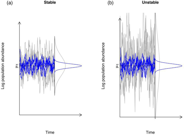
Figure 1.

The abundances in stable (a) vs. unstable (b) populations. In both panels the grey lines represent the log-population abundances at stationarity were simulated under the stochastic Gompertz model of Ponciano et al. (2018) under the same environmental noise regime that are shown in blue. The variance of the long run log-population abundances is equal to the ratio of the environmental noise variance (here 0.11) to one minus the squared strength of density-dependence c. This coefficient is stronger on the left than on the right. On the left c = 0.75 and so the log-population size variance is 0.11/(1−0.75²) = 0.2514. On the right panel, density dependence is much weaker, with a coefficient equal to 0.93. (Coefficients closer to 1 are close to density-independence.) The variance of the population abundances under the same environmental noise variance is approximately three times higher: 0.11/(1 − 0.93²) = 0.8142. The magnitude of the response of a population to environmental noise, in terms of variability, is modulated by c.