Designing individually randomized group treatment trials with repeated outcome measurements using generalized estimating equations

Abstract

Individually randomized group treatment (IRGT) trials, in which the clustering of outcome is induced by group-based treatment delivery, are increasingly popular in public health research. IRGT trials frequently incorporate longitudinal measurements, of which the proper sample size calculations should account for correlation structures reflecting both the treatment-induced clustering and repeated outcome measurements. Given the relatively sparse literature on designing longitudinal IRGT trials, we propose sample size procedures for continuous and binary outcomes based on the generalized estimating equations approach, employing the block exchangeable correlation structures with different correlation parameters for the treatment arm and for the control arm, and surveying 5 marginal mean models with different assumptions of time effect: no-time constant treatment effect, linear-time constant treatment effect, categorical-time constant treatment effect, linear time by treatment interaction, and categorical time by treatment interaction. Closed-form sample size formulas are derived for continuous outcomes, which depends on the eigenvalues of the correlation matrices; detailed numerical sample size procedures are proposed for binary outcomes. Through simulations, we demonstrate that the empirical power agrees well with the predicted power, for as few as 8 groups formed in the treatment arm, when data are analyzed using the matrix-adjusted estimating equations for the correlation parameters with a bias-corrected sandwich variance estimator.

1 |. INTRODUCTION

Individually randomized group treatment (IRGT) trials (also referred to as individually randomized trials with post-randomization clustering which can involve differential clustering in different trial arms) are becoming increasingly popular in public health research and biomedical studies.^1,2,3 In an IRGT trial, although individuals are randomized to different trial arms, clustering of outcomes arises in one or both conditions due to the nature of the treatment being either group-based (e.g. a group-based psychological treatment) or delivered to multiple participants by the same individual (e.g. surgeon). In some IRGT trials, no clustering of outcomes occurs in the control or usual care condition.^4,5 Reasons for the group treatment include cost savings over individual treatment delivery and prevention of contamination, among others.^6,7 Due to post-randomization clustering, IRGT trials differ from traditional individually randomized controlled trials (RCTs) in which outcomes of individuals within each trial arm are assumed independent. In contrast to cluster randomized trials (CRTs) for which clusters are typically pre-existing organizations or groups (such as clinics or hospitals), IRGT trials necessitate randomization at the individual level but form clusters after randomization is carried out. Whereas clustering of outcomes is usually expected to be same in both arms in CRTs (with a few exceptions⁸), the clustering of outcomes is expected to be different between arms in IRGT trials depending on the nature and context of the treatment conditions.

For IRGT trials, given that clustering of outcomes typically exists among individuals within the treatment arm but may not be present within the control arm, there can be different levels of hierarchy for the two arms, for example with an additional level in the treatment arm compared to the control arm. In this case, statistical modeling and sample size calculations for such trials should consider different correlation structures for different arms, as first discussed by Roberts and Roberts.⁴ Methods for designing and analyzing standard IRGT trials have been developed in previous studies, i.e. for IRGT trials with outcome measurements at a single follow-up time point and clustering only in the treatment arm, resulting in a two-level structure in the treatment arm and a one-level structure in the control arm. These methods often include mixed-effects models and marginal models fitted by the generalized estimating equations. For example, Bauer et al.⁵ presented several mixed-effects models for data analysis with a focus on testing the treatment effect, and Baldwin et al.⁹ evaluated the performance of these models through simulations by type I error rate, bias, efficiency, and power. Assuming a linear mixed model, Roberts and Roberts⁴ developed sample size calculations for a continuous outcome at a single time point, Moerbeek and Wong¹⁰ derived closed-form sample size formulas for continuous and binary outcomes with outcomes measured at a single time point, Candel and Van Breukelen¹¹ extended these results to unequal cluster sizes based on a linear mixed model with a continuous outcome, and recently, Teerenstra et al.¹² incorporated an unclustered baseline measure for a continuous outcome at a single follow-up time point.

Similar to traditional individually randomized trials, IRGT trials can also incorporate repeated outcome measurements. That is, outcomes are measured on each individual at repeated follow-up time points, so that an additional level of nesting should be considered in each arm. Therefore, in the case of a standard IRGT trial with no clustering due to group-based care delivery in the control arm, the levels of hierarchy for the treatment and control arms would be three and two, respectively. More generally, the levels of hierarchy for the treatment and control arms would both be three, but with different degrees of clustering or different correlation parameters. We collectively refer to this type of design as the “longitudinal individually randomized group treatment trial” or longitudinal IRGT trial. An example of such a longitudinal IRGT trial is the Sauti ya Vijana (SYV, The Voice of Youth) trial which is in its design phase at the time of writing. The goal of this trial is to assess the impact of the SYV psychosocial and life-skills treatment to improve HIV outcomes in Tanzanian youth. Individuals are randomized into the treatment or control arm, and the treatment condition is a series of group-based mental health sessions, while the control condition is routine care as usual delivered individually. An outcome of interest is the log viral load assessed at 3 follow-up time points. Figure 1 provides a hierarchical illustration of the SYV trial with three levels for the treatment arm and two levels for the control arm.

FIGURE 1.

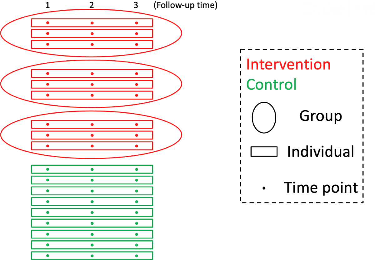
An illustration of the SYV trial, a longitudinal individually randomized group treatment trial with 9 individuals per arm, 3 individuals per group in the treatment arm, no treatment-induced clustering of individuals in the control arm, and 3 follow-up time points per individual.

Despite these existing developments assuming outcomes measured at a single time point, the availability of methods for designing longitudinal IRGT trials is limited. To the best of our knowledge, there are only two studies addressing challenges in designing longitudinal IRGT trials. Heo et al.² considered a two-level and a three-level linear mixed model to derive sample size formulas for multilevel IRGT trials, but considered relatively simple correlation structures and did not address fixed time-effects that may be present in longitudinal IRGT trials. Esserman et al.¹³ considered a linear mixed model with linear time trend and treatment-by-time interaction to derive a sample size formula for longitudinal IRGT trials, but also restricted to relatively simple within-cluster correlation structures. Both studies have only considered a continuous outcome variable, where as binary outcomes can also be common in IRGT trials. A brief summary of existing literature for designing IRGT trials is presented in Table 1 . To account for multiple levels of clustering in longitudinal IRGT trials, both marginal (population-averaged) and conditional (group-specific) models can be used. A major distinction between marginal and conditional models is the interpretation of the regression parameters, although the distinction is immaterial when considering collapsible link functions.^14,15 In a marginal model, the treatment effect describes the difference of average response between the subsets of the population defined by treatment and control. In a conditional model, the treatment effect describes the difference of average response between treatment and control conditional on the latent, unobserved random effect describing the cluster or group. Accordingly, marginal models may be preferred for their population-averaged interpretations in comparing group-delivered treatments.^16,17 However, to the best of our knowledge, existing methods for IRGT trials including those incorporating a longitudinal component are all based on linear mixed models, or conditional models (as summarized in Table 1). In this article, we hence focus on sample size development for longitudinal IRGT trials with continuous and binary outcomes based on the marginal model. To allow for generality, we consider the levels of hierarchy for the treatment and control arms are both three, but assume differential correlation parameters in the two arms to account for different degrees of clustering; this includes, as a special case, designs where the levels of hierarchy for the treatment and control arms are three and two, respectively. We characterize sample size procedures under 5 marginal mean models with different assumptions of time effect: no-time constant treatment effect, linear-time constant treatment effect, categorical-time constant treatment effect, linear time by treatment interaction, and categorical time by treatment interaction. We conduct a simulation study to assess the validity of the proposed sample size formulas, and apply our method to the design of the motivating SYV trial.

TABLE 1.

Brief summary of existing literature for designing IRGT trials.

Reference	Modela	Allow for Longitudinal Outcomesb	Outcome Type
Roberts and Roberts (2005)4	LMM	No	Continuous
Moerbeek and Wong (2008)10	LMM	No	Continuous
			Binary
Candel and Van Breukelen (2009)11	LMM	No	Continuous
Esserman et al. (2013)13	LMM	Yes	Continuous
Heo et al. (2017)2	LMM	Yes	Continuous

^aLMM: linear mixed model.

^bDefined as a trial with outcomes measured at more than one follow-up time point.

2 |. ANALYSIS OF LONGITUDINAL IRGT TRIALS USING GENERALIZED ESTIMATING EQUATIONS

For the treatment arm, let $Y_{ijk}$ denote the outcome for individual $k=1,\dots ,K_i$ in cluster (i.e. group, and in what follows we use groups and clusters interchangeably) $i=1,\dots ,I_t$ at follow-up time point $j=1,\dots ,T$. Here we assume all time points to be follow-up time points, i.e., after randomization, so that we do not require any constrained longitudinal data analysis whereby we posit equal mean outcome levels in the two arms at baseline.¹⁸ For simplicity, we assume that all clusters in the treatment arm have the same size, i.e. $K_i=K_t\left(i=1,\dots ,I_t\right)$. Similarly, for the control arm, let $Y_{ijk}$ denote the continuous or binary outcome for individual $k=1,\dots ,K_i$ in cluster (i.e. group) $i=I_t+1,\dots ,I_t+I_c$ at time point $j=1,\dots ,T$, and assume that all clusters in the control arm have the same size, i.e. $K_i=K_c\left(i=I_t+1,\dots ,I_t+I_c\right)$. Let $I=I_t+I_c$ be the total number of clusters, $N_t=I_t\times K_t$ be the total number of individuals in the treatment arm, $N_c=I_c\times K_c$ be the total number of individuals in the control arm, $N=N_t+N_c$ be the total number of individuals, ${\pi }_c=N_c/N$ be the proportion of individuals randomized to the control arm, and $q_c=I_c/I$ be the proportion of clusters in the control arm. Then the total number of individuals can be expressed as $N=I\times \left\{q_c{K}_c+\left(1-q_c\right)K_t\right\}$. Let $X_i$ denote a binary treatment indicator, ${\mathit{X}}_{ijk}={\left(X_{ijk1},\dots ,X_{ijkp}\right)}^{\prime }$ denote a list of $p$ covariates including $X_i$. Let ${\mu }_{ijk}=E\left(Y_{ijk}\mid {\mathit{X}}_{ijk}\right)$ be the marginal mean outcome given ${\mathit{X}}_{ijk}$, which is specified via a generalized linear model

$$g\left({\mu }_{ijk}\right)={\mathit{X}}_{ijk}^{\prime }\mathit{\beta },$$ (1)

where $g$ is a link function and $\mathit{\beta }$ is a $p\times 1$ vector of regression parameters. The marginal variance function is specified as $\mathrm{V}\mathrm{a}\mathrm{r}\left(Y_{ijk}\mid X_{ijk}\right)={\varphi }_i{v}_{ijk}$ with ${\varphi }_i={\varphi }_t$ for $i$ in the treatment arm and ${\varphi }_i={\varphi }_c$ for $i$ in the control arm, where ${\varphi }_t$ and ${\varphi }_c$ are the dispersion parameters to allow for the heteroscedasticity for continuous outcomes, and $v_{ijk}$ is a variance function that could depend on the marginal mean.

For each cluster, denote ${\mathit{Y}}_i={\left(Y_{i11},Y_{i12},\dots ,Y_{iT{K}_i}\right)}^{\prime }$, ${\mathit{\mu }}_i={\left({\mu }_{i11},{\mu }_{i12},\dots ,{\mu }_{iT{K}_i}\right)}^{\prime }$, where ${\mathit{Y}}_i$ and ${\mathit{\mu }}_i$ are of dimension $T{K}_i$; denote ${\mathit{X}}_i$ as the $T{K}_i\times p$ covariate matrix. For the treatment arm, we assume the degree of similarity among the within-cluster outcomes is characterized through the block exchangeable correlation structure,¹⁹ with the following assumptions:

1. the within-time correlation for two different individuals in the same cluster is ${\alpha }_0:\mathrm{c}\mathrm{o}\mathrm{r}\mathrm{r}\left(Y_{ijk},Y_{ij{k}^{\prime }}\right)={\alpha }_0$ for $k\ne k^{\prime }$;

2. the between-time correlation for two different individuals in the same cluster is ${\alpha }_1:\mathrm{c}\mathrm{o}\mathrm{r}\mathrm{r}\left(Y_{ijk},Y_{i{j}^{\prime }{k}^{\prime }}\right)={\alpha }_1$ for $j\ne j^{\prime }$ and $k\ne k^{\prime }$;

3. the within-individual correlation is ${\alpha }_2:\mathrm{c}\mathrm{o}\mathrm{r}\mathrm{r}\left(Y_{ijk},Y_{i{j}^{\prime }k}\right)={\alpha }_2$ for $j\ne j^{\prime }$.

Of note, this block exchangeable correlation structure has been previously used in a closed-cohort stepped wedge CRT with repeated outcome assessments at the individual level.²⁰ Similarly, for the control arm, we assume the degree of similarity among the within-cluster outcomes is also characterized through the block exchangeable correlation structure,¹⁹ but with potentially different correlation parameters:

1. the within-time correlation for two different individuals in the same cluster is ${\rho }_0:\mathrm{c}\mathrm{o}\mathrm{r}\mathrm{r}\left(Y_{ijk},Y_{ij{k}^{\prime }}\right)={\rho }_0$ for $k\ne k^{\prime }$;

2. the between-time correlation for two different individuals in the same cluster is ${\rho }_1:\mathrm{c}\mathrm{o}\mathrm{r}\mathrm{r}\left(Y_{ijk},Y_{i{j}^{\prime }{k}^{\prime }}\right)={\rho }_1$ for $j\ne j^{\prime }$ and $k\ne k^{\prime }$;

3. the within-individual correlation is ${\rho }_2:\mathrm{c}\mathrm{o}\mathrm{r}\mathrm{r}\left(Y_{ijk},Y_{i{j}^{\prime }k}\right)={\rho }_2$ for $j\ne j^{\prime }$.

That is, we allow for differential clustering in the two arms. For example, in practice, the within-individual correlation could be different between the two arms if the treatment leads to greater consistency of outcomes within an individual over time. As an important special case, setting ${\rho }_0={\rho }_1=0$ corresponds to the scenario where there is treatment-induced clustering only in the treatment arm but none in the control arm. This special case is a longitudinal generalization of the partially nested design, and reflects the complication in our motivating SYV trial. In what follows, we will develop our methodology for the general case, but focus on the special case with ${\rho }_0={\rho }_1=0$ in our numerical studies.

2.1 |. Generalized estimating equations

We use the generalized estimating equations (GEE) approach²¹ to estimate the parameters in mean model (1). Define ${\mathit{D}}_i=\partial {\mathit{\mu }}_i/\partial {\mathit{\beta }}^{\prime }$, and let ${\mathit{V}}_i={\mathit{A}}_i^{1/2}{\mathit{R}}_i{\mathit{A}}_i^{1/2}$ be a working covariance matrix for ${\mathit{Y}}_i$, where ${\mathit{A}}_i$ is a $T{K}_i$-dimensional diagonal matrix with elements of ${\varphi }_i{v}_{ijk}$, and ${\mathit{R}}_i={\mathit{R}}_i(\mathit{\alpha },\mathit{\rho })$ is a working correlation matrix specified by the intraclass correlation coefficient (ICC) vector $(\mathit{\alpha },\mathit{\rho })={\left({\alpha }_0,{\alpha }_1,{\alpha }_2,{\rho }_0,{\rho }_1,{\rho }_2\right)}^{\prime }$. We denote ${\mathit{I}}_s$ and ${\mathit{J}}_s$ as the $s\times s$ identity matrix and matrix of ones, respectively. According to Li et al.,¹⁹ the block exchangeable correlation structure within the treatment arm can be expressed as

$${\mathit{R}}_t=\left(1-{\alpha }_0+{\alpha }_1-{\alpha }_2\right){\mathit{I}}_{T{K}_t}+\left({\alpha }_2-{\alpha }_1\right){\mathit{J}}_T\otimes {\mathit{I}}_{K_t}+\left({\alpha }_0-{\alpha }_1\right){\mathit{I}}_T\otimes {\mathit{J}}_{K_t}+{\alpha }_1{\mathit{J}}_{T{K}_t},$$

which has the following four distinct eigenvalues:

$$\begin{array}{l}{\lambda }_{t1}=1-{\alpha }_0+{\alpha }_1-{\alpha }_2,\\ {\lambda }_{t2}=1-{\alpha }_0-(T-1)\left({\alpha }_1-{\alpha }_2\right),\\ {\lambda }_{t3}=1+\left(K_t-1\right)\left({\alpha }_0-{\alpha }_1\right)-{\alpha }_2,\\ {\lambda }_{t4}=1+\left(K_t-1\right){\alpha }_0+(T-1)\left(K_t-1\right){\alpha }_1+(T-1){\alpha }_2.\end{array}$$ (2)

The combinations of $\left({\alpha }_0,{\alpha }_1,{\alpha }_2\right)$ to ensure a positive definite ${\mathit{R}}_t$ can be efficiently determined by $\mathrm{m}\mathrm{i}\mathrm{n}\left\{{\lambda }_{t1},{\lambda }_{t2},{\lambda }_{t3},{\lambda }_{t4}\right\}>0$. Similarly, the block exchangeable correlation structure within the control arm can be expressed as

$${\mathit{R}}_c=\left(1-{\rho }_0+{\rho }_1-{\rho }_2\right){\mathit{I}}_{T{K}_c}+\left({\rho }_2-{\rho }_1\right){\mathit{J}}_T\otimes {\mathit{I}}_{K_c}+\left({\rho }_0-{\rho }_1\right){\mathit{I}}_T\otimes {\mathit{J}}_{K_c}+{\rho }_1{\mathit{J}}_{T{K}_c},$$

which has the following four distinct eigenvalues:

$$\begin{array}{l}{\lambda }_{c1}=1-{\rho }_0+{\rho }_1-{\rho }_2,\\ {\lambda }_{c2}=1-{\rho }_0-(T-1)\left({\rho }_1-{\rho }_2\right),\\ {\lambda }_{c3}=1+\left(K_c-1\right)\left({\rho }_0-{\rho }_1\right)-{\rho }_2,\\ {\lambda }_{c4}=1+\left(K_c-1\right){\rho }_0+(T-1)\left(K_c-1\right){\rho }_1+(T-1){\rho }_2.\end{array}$$ (3)

Again, the combinations of $\left({\rho }_0,{\rho }_1,{\rho }_2\right)$ to ensure a positive definite ${\mathit{R}}_c$ can be efficiently determined by $\mathrm{m}\mathrm{i}\mathrm{n}\left\{{\lambda }_{c1},{\lambda }_{c2},{\lambda }_{c3},{\lambda }_{c4}\right\}>0$.

The GEE estimator $\stackrel{\mathit{ˆ}}{\mathit{\beta }}$ is obtained by solving the $\mathit{\beta }$-estimating equations ${\sum }_{i=1}^I {\mathit{D}}_i^{\prime }{\mathit{V}}_i^{-1}\left({\mathit{Y}}_i-{\mathit{\mu }}_t\right)=\mathbf{0}$. Asymptotically, $I^{1/2}(\stackrel{\mathit{ˆ}}{\mathit{\beta }}-\mathit{\beta })$ is multivariate normal with mean 0 and covariance estimated by the model-based variance estimator

$${\mathit{V}}_R^{\mathrm{m}\mathrm{o}\mathrm{d}\mathrm{e}\mathrm{l}}={\stackrel{\mathbf{ˆ}}{\mathbf{\Sigma }}}_1^{-1}={\left(I^{-1}\sum _{i=1}^I {\mathit{D}}_i^{\prime }(\stackrel{\mathit{ˆ}}{\mathit{\beta }}){\mathit{V}}_i^{-1}(\stackrel{\mathit{ˆ}}{\mathit{\alpha }},\stackrel{\mathit{ˆ}}{\mathit{\rho }}){\mathit{D}}_i(\stackrel{\mathit{ˆ}}{\mathit{\beta }})\right)}^{-1}$$

or by the sandwich variance estimator ${\mathit{V}}_R^{\text{sandwich}}={\stackrel{\mathbf{ˆ}}{\mathbf{\Sigma }}}_1^{-1}{\stackrel{\mathbf{ˆ}}{\mathbf{\Sigma }}}_0{\stackrel{\mathbf{ˆ}}{\mathbf{\Sigma }}}_1^{-1}$, where

$${\stackrel{\mathbf{ˆ}}{\mathbf{\Sigma }}}_0=I^{-1}\sum _{i=1}^I C_i{\mathit{D}}_i^{\prime }(\stackrel{\mathit{ˆ}}{\mathit{\beta }}){\mathit{V}}_i^{-1}\left(\stackrel{\mathit{ˆ}}{\mathit{\alpha }},\stackrel{\mathit{ˆ}}{\mathit{\rho }}\right)\left({\mathit{Y}}_i-{\hat{\mathit{\mu }}}_i\right){\left({\mathit{Y}}_i-{\hat{\mu }}_i\right)}^{\prime }{\mathit{V}}_i^{-1}\left(\stackrel{\mathrm{ˆ}}{\mathit{\alpha }},\hat{\mathit{\rho }}\right){\mathit{D}}_i(\stackrel{\mathit{ˆ}}{\mathit{\beta }}){\mathit{C}}_i^{\prime },$$ (4)

and ${\mathit{C}}_i$ is a cluster-specific matrix for negative bias correction in variance estimation for small samples, following Wang et al.²² The sandwich variance estimator is asymptotically valid regardless of the correct specification of the working correlation structure ${\mathit{R}}_i$, while the consistency of the model-based variance requires the correct specification of ${\mathit{R}}_i$. In Equation (4), setting ${\mathit{C}}_i={\mathit{I}}_p$ gives the uncorrected robust sandwich variance estimator of Liang and Zeger,²¹ denoted as ROB. When the number of clusters is small, ROB tends to underestimate the variance and inflate the type I error rate.^23,24 We consider 2 types of small-sample bias corrections. Defining ${\mathit{Q}}_i={\mathit{D}}_i^{\prime }{\mathit{V}}_i^{-1}{\mathit{D}}_i{\left(I{\mathbf{\Sigma }}_1\right)}^{-1}$, the bias-corrected sandwich variance estimator of Kauermann and Carroll²³ is given by setting ${\mathit{C}}_i={\left\{{\mathit{I}}_p-{\mathit{Q}}_i\right\}}^{-1/2}$, denoted as KC; the bias-corrected sandwich variance estimator of Mancl and DeRouen²⁵ is given by setting ${\mathit{C}}_i={\left\{{\mathit{I}}_p-{\mathit{Q}}_i\right\}}^{-1}$, denoted as MD.

2.2 |. Matrix-adjusted estimating equations

In addition to using GEE to estimate the marginal mean model parameters, we also consider an additional set of estimating equations, specifically the matrix-adjusted estimating equations (MAEE) of Preisser et al.,¹⁵ to estimate $(\mathit{\alpha },\mathit{\rho })$. Compared to the usual second-order estimating equations provided in Prentice,²⁶ MAEE is particularly appealing in this context because it provides more accurate estimates for the correlation parameters in finite samples (especially when the number of clusters is small), and the values of such correlation parameters are of interest for the design of future IRGT trials.^15,27 We provide a brief overview of MAEE below. Without loss of clarity, for each pair of outcomes $l$ and $l^{\prime }$ in cluster $i$ (i.e. combining the $j$ and $k$ indices into $l:1\le l,l^{\prime }\le T{K}_i$ for $i=1,\dots ,I_t,I_t+1,\dots ,I$), write

$${\eta }_{il{l}^{\prime }}\left({\mu }_{il},{\mu }_{i{l}^{\prime }},{\varphi }_i\right)=\frac{\left(Y_{il}-{\mu }_{il}\right)\left(Y_{i{l}^{\prime }}-{\mu }_{i{l}^{\prime }}\right)}{{\varphi }_i{v}^{1/2}\left({\mu }_{il}\right)v^{1/2}\left({\mu }_{i{l}^{\prime }}\right)}.$$

For $l=l^{\prime }$, ${\eta }_{il{l}^{\prime }}$ is interpreted as the sample standardized residual; for $l\ne l^{\prime }$, ${\eta }_{il{l}^{\prime }}$ is interpreted as the sample correlation.

If $Y_{il}$ is binary with ${\varphi }_t={\varphi }_c=1$, for $l\ne l^{\prime }$, Prentice²⁶ has shown that $E\left({\eta }_{il{l}^{\prime }}\right)={\zeta }_{il{l}^{\prime }}$ and

$$\mathrm{V}\mathrm{a}\mathrm{r}\left({\eta }_{il{l}^{\prime }}\right)=z_{il{l}^{\prime }}=1+\frac{\left(1-2{\mu }_{il}\right)\left(1-2{\mu }_{i{l}^{\prime }}\right){\zeta }_{il{l}^{\prime }}}{{\left\{{\mu }_{il}{\mu }_{i{l}^{\prime }}\left(1-{\mu }_{il}\right)\left(1-{\mu }_{i{l}^{\prime }}\right)\right\}}^{1/2}}-{\zeta }_{il{l}^{\prime }}^2,$$

where ${\zeta }_{il{l}^{\prime }}$ is the ICC parameter as the $\left(l,l^{\prime }\right)$ th element of ${\mathit{R}}_i$. In a longitudinal IRGT trial, ${\zeta }_{il{l}^{\prime }}={\zeta }_{il{l}^{\prime }}(\mathit{\alpha },\mathit{\rho })$ is a function of $\mathit{\alpha }$ or $\mathit{\rho }$, and is equal to one element of $\left\{{\alpha }_0,{\alpha }_1,{\alpha }_2,{\rho }_0,{\rho }_1,{\rho }_2\right\}$ depending on $i$ and the coordinate pair $\left(l,l^{\prime }\right)$. For each cluster $i$, define ${\mathit{\zeta }}_i={\left({\zeta }_{i12},{\zeta }_{i13},\dots ,{\zeta }_{i,\left(T{K}_i-1\right),T{K}_i}\right)}^{\prime }$, ${\mathit{E}}_i=\partial {\mathit{\zeta }}_i/\partial \left({\mathit{\alpha }}^{\prime },{\mathit{\rho }}^{\prime }\right)$, and ${\mathit{Z}}_i=\mathrm{d}\mathrm{i}\mathrm{a}\mathrm{g}\left(z_{i12},z_{i13},\dots ,z_{i,\left(T{K}_i-1\right),T{K}_i}\right)$. Then the matrix-adjusted $(\mathit{\alpha },\mathit{\rho })$-estimating equations¹⁵ are

$$\sum _{i=1}^I{\mathit{E}}_i^{\prime }{\mathit{Z}}_i^{-1}\left({\tilde{\mathit{\eta }}}_i-{\mathit{\zeta }}_i\left(\mathit{\alpha },\mathit{\rho }\right)\right)=\mathbf{0},$$ (5)

where ${\tilde{\mathit{\eta }}}_i={({\tilde{\mathit{\eta }}}_{i12},{\tilde{\mathit{\eta }}}_{i13},\dots ,{\tilde{\mathit{\eta }}}_{i,\left(T{K}_i-1\right),T{K}_i})}^{\prime }$ is a vector of bias-corrected sample correlations with elements

$${\tilde{\eta }}_{il{l}^{\prime }}={\left[{\mathit{A}}_i^{-1/2}{\left(\mathit{I}-{\mathit{H}}_i\right)}^{-1}{\mathit{A}}_i^{1/2}\right]}_{l\cdot }{\left[{\stackrel{\mathit{ˆ}}{\mathit{R}}}_i\right]}_{{\cdot l}^{\prime }},$$

$[\mathit{M}{]}_{l\cdot }$ and $[\mathit{M}{]}_{\cdot l^{\prime }}$ are the lth row and l′th column of the matrix $\mathit{M}$, respectively, ${\mathit{H}}_i$ is the ith cluster leverage,²⁸ and ${\stackrel{\mathit{ˆ}}{\mathit{R}}}_i$ is the estimated working correlation matrix with element ${\eta }_{il{l}^{\prime }}\left({\hat{\mu }}_{il},{\hat{\mu }}_{i{l}^{\prime }},{\varphi }_t={\varphi }_c=1\right)$. The GEE/MAEE estimators $\stackrel{\mathit{ˆ}}{\mathit{\beta }}$ and $(\stackrel{\mathit{ˆ}}{\mathit{\alpha }},\stackrel{\mathit{ˆ}}{\mathit{\rho }})$ are obtained by solving the $\mathit{\beta }$-estimating equations and $(\mathit{\alpha },\mathit{\rho })$-estimating equations iteratively, with detailed steps provided in Prentice.²⁶

If $Y_{il}$ is continuous, we assume a Gaussian model with $v_{ijk}=1$. For $l\ne l^{\prime }$, Li et al.¹⁹ has shown that $E\left({\eta }_{il{l}^{\prime }}\right)={\zeta }_{il{l}^{\prime }}$ and

$$\mathrm{Var}\left({\eta }_{il{l}^{\prime }}\right)=z_{il{l}^{\prime }}=1+{\zeta }_{il{l}^{\prime }}^2.$$

The matrix-adjusted $(\mathit{\alpha },\mathit{\rho })$-estimating equations (5) will be used to estimate the ICC parameters, with $z_{il{l}^{\prime }}$ defined above and

$${\tilde{\eta }}_{il{l}^{\prime }}={\left[{\left(\mathit{I}-{\mathit{H}}_i\right)}^{-1}\right]}_{l\cdot }{\left[{\stackrel{\mathit{ˆ}}{\mathit{R}}}_i\right]}_{\cdot l^{\prime }},$$

because ${\mathit{A}}_i={\varphi }_i\mathit{I}$ doesn’t depend on the marginal mean parameters. Similar to the binary outcome case, GEE/MAEE estimators can be obtained by solving the $\mathit{\beta }$-estimating equations and $(\mathit{\alpha },\mathit{\rho })$-estimating equations iteratively, with an additional step in the procedure to update the nuisance parameters ${\varphi }_t$ and ${\varphi }_c$. Following similar steps outlined in Li et al.,¹⁹ from iteration $s$ to $s+1$, the updating formulas are provided as ${\hat{\varphi }}_t^{(s+1)}={\hat{\varphi }}_t^{\left(s\right)}{\sum }_{i=1}^{I_t} {\sum }_{l=1}^{T{K}_t} {\tilde{\eta }}_{ill}/\left(I_{t}T{K}_t-p\right)$ and ${\hat{\varphi }}_c^{(s+1)}={\hat{\varphi }}_c^{\left(s\right)}{\sum }_{i=1}^{I_c} {\sum }_{l=1}^{T{K}_c} {\tilde{\eta }}_{ill}/\left(I_{c}T{K}_c-p\right)$ (essentially estimating ${\varphi }_t$ and ${\varphi }_c$ separately within each arm).

3 |. POWER AND SAMPLE SIZE CONSIDERATIONS

As longitudinal IRGT trials collect multiple outcome observations for each individual, and can be analyzed by more than one marginal mean model, we consider an overarching research question of testing the existence of any global treatment effect as a common basis for assessing our sample size methods. When obtaining the variance of treatment effect estimator, we assume the mean model (1) is correct such that the treatment effect parameters can be well-defined. We first introduce two testing paradigms that are associated with our sample size methods, before presenting specific sample size considerations for each marginal mean model specification.

3.1 |. Testing a single parameter

Suppose that we are interested in testing the null hypothesis of $H_0:{\beta }_p=0$, using a two-sided t-test. Specifically, based on mean model (1), the asymptotic distribution of $\sqrt{I}({\hat{\beta }}_p-{\beta }_p)$ is normal with mean 0 and variance obtained as the $(p,p)$th element of $\mathrm{c}\mathrm{o}\mathrm{v}\{\sqrt{I}(\stackrel{\mathit{ˆ}}{\mathit{\beta }}-\mathit{\beta })\}$. The Wald test statistic $\sqrt{I}{\hat{\beta }}_p/{\sigma }_{\beta }$, where ${\sigma }_{\beta }^2=\mathrm{v}\mathrm{a}\mathrm{r}(\sqrt{I}{\hat{\beta }}_p)$, will be compared to a $t$-distribution with $df$ degrees of freedom (for example, a common choice is $df=I-p$ to account for small-sample biases and to maintain valid type I error rate); the t-test is adopted since it often performs better in finite samples than normal approximations.^29,22 Asymptotically, the power to detect an effect ${\beta }_p$ of size $b$ with a nominal two-sided type I error rate $\alpha$ is

$$1-\gamma ={\mathrm{\Phi }}_{t,df}\left(t_{\alpha /2,df}+|b|\sqrt{\frac{I}{{\sigma }_{\beta }^2}}\right),$$ (6)

where ${\mathrm{\Phi }}_{t,df}$ and $t_{\alpha ,df}$ are the cumulative distribution function and $100\alpha \mathrm{\%}$ percentile of the $t$-distribution with $df$ degrees of freedom. Then the number of individuals required to achieve $100(1-\gamma )\mathrm{\%}$ power must satisfy

$$N\ge {\left(t_{\alpha /2,df}+t_{\gamma ,df}\right)}^2\frac{{\sigma }_{\beta }^2}{b^2}\times \left\{q_c{K}_c+\left(1-q_c\right)K_t\right\}.$$ (7)

From Equations (6) and (7), the analytical power and sample size calculations rely on an explicit form of the asymptotic variance ${\sigma }_{\beta }^2$. Assuming that the true correlation matrix of ${\mathit{Y}}_i$ is block exchangeable with different parameters in different arms, we derive the expression of ${\sigma }_{\beta }^2$ using the true working correlation structures or using an independence working correlation structure in the subsequent sections.

3.2 |. Testing multiple parameters

Let ${\mathit{\beta }}_{sub}={\left({\beta }_q,\dots ,{\beta }_p\right)}^{\prime }$, where $1\le q<p$, and ${\mathit{h}}_0=(0,\dots ,0{)}^{\prime }$ be two vectors of length $r=p-q+1$. Suppose we are interested in testing the null hypothesis of ${\mathit{H}}_0:{\mathit{\beta }}_{sub}={\mathit{h}}_0$, versus the alternative hypothesis of ${\mathit{H}}_1$ : at least one element of ${\mathit{\beta }}_{sub}$ is not 0. Here we are testing multiple parameters but not just a single parameter for the treatment effect, and all the parameters to test need to be arranged from the qth to the pth position. Note that this is useful when time-by-treatment interactions are of interest, and will be considered further in Section 3.3. Denote ${\mathit{V}}_{sub}$ as the lower-right block of $\mathrm{c}\mathrm{o}\mathrm{v}\{\sqrt{I}(\stackrel{\mathit{ˆ}}{\mathit{\beta }}-\mathit{\beta })\}$ with dimension $r\times r$.

Then the $F$-test statistic

$$F^{\mathrm{*}}=\frac{I{\left({\stackrel{\mathit{ˆ}}{\mathit{\beta }}}_{sub}-{\mathit{h}}_0\right)}^{\prime }{\mathit{V}}_{sub}^{-1}\left({\stackrel{\mathit{ˆ}}{\mathit{\beta }}}_{sub}-{\mathit{h}}_0\right)}{r}$$

asymptotically follows a non-central $F(\lambda ;r,\nu )$ distribution, with non-centrality parameter

$$\lambda \approx I{\left({\stackrel{\mathit{ˆ}}{\mathit{\beta }}}_{sub}-{\mathit{h}}_0\right)}^{\prime }{\mathit{V}}_{sub}^{-1}\left({\stackrel{\mathit{ˆ}}{\mathit{\beta }}}_{sub}-{\mathit{h}}_0\right),$$ (8)

and degrees of freedom $r$ and $v$, where $v=I-(r+1)$ is an approximation of the denominator degrees of freedom. Thus, if $\alpha$ represents the type I error rate and $F_{1-\alpha }(r,v)$ is the critical value from the central $F(r,v)$ distribution, the power associated with $Q_W$ is given by

$$1-\gamma ={\int }_{F_{1-\alpha }(r,v)}^{\mathrm{\infty }} f(x;\lambda ,r,v)\mathrm{d}x$$ (9)

where $\gamma$ is the type II error rate and $f(x;\lambda ,r,\nu )$ is the probability density function of the non-central $F(\lambda ;r,\nu )$ distribution.

Accordingly, the number of individuals required to achieve $100(1-\gamma )\mathrm{\%}$ power, to detect an effect of size ${\mathit{b}}_{sub}={\left(b_q,\dots ,b_p\right)}^{\prime }$, must satisfy

$$N\ge \frac{\lambda }{{\left({\mathit{b}}_{sub}-{\mathit{h}}_0\right)}^{\prime }{\left[{\mathit{V}}_{sub}\right]}^{-1}\left({\mathit{b}}_{sub}-{\mathit{h}}_0\right)}\times \left\{q_c{K}_c+\left(1-q_c\right)K_t\right\},$$ (10)

where $\lambda$ is determined by iteratively solving (8) and (9) for the given values of $\alpha$ and $\gamma$. Equations (8) and (10) suggest that analytical power and sample size calculations depend on an explicit expression for the asymptotic variance ${\mathit{V}}_{sub}$. Again, assuming that the true correlation matrix of ${\mathit{Y}}_i$ is block exchangeable with different parameters in different arms, we derive the expression of ${\mathit{V}}_{sub}$ using the true working correlation structures or using an independence working correlation structure in the subsequent sections for appropriate models that require a multi-parameter test.

3.3 |. Using the model-based variance with a continuous outcome

When $Y_{ijk}$ is continuous, we have the variance function $v_{ijk}=1$. In this section, to determine the explicit form of ${\sigma }_{\beta }^2$ or ${\mathit{V}}_{sub}$, we assume that the working correlation matrix is block exchangeable for each arm (with different correlation parameters), with correlation parameters estimated through the MAEE approach.

3.3.1 |. Model 1: No-time constant treatment effect model (NT-CTE)

Assuming there is no time effect, the marginal mean model (1) is

$${\mu }_{ijk}={\beta }_1+{\beta }_2{X}_i.$$

Suppose that we are interested in testing the null hypothesis of no treatment effect $H_0:{\beta }_2=0$ with $df=I-2,$²⁵ using the procedure stated in Section 3.1. For clusters in the control arm, ${\mathit{X}}_i={\mathit{X}}_c=\left({\mathbf{1}}_{T{K}_c},{\mathbf{0}}_{T{K}_c}\right)$; for clusters in the treatment arm, ${\mathit{X}}_i={\mathit{X}}_t=\left({\mathbf{1}}_{T{K}_t},{\mathbf{1}}_{T{K}_t}\right)$. Then ${\sigma }_{\beta }^2=\mathrm{v}\mathrm{a}\mathrm{r}(\sqrt{I}{\hat{\beta }}_2)$ is the lower-right element of ${\mathit{V}}_R^{\text{model}}$, given by the inverse of

$$\begin{array}{l}{\mathbf{\Sigma }}_1=I^{-1}\sum _{i=1}^I {\mathit{D}}_i^{\prime }{\mathit{V}}_i^{-1}{\mathit{D}}_i=I^{-1}\left(I_c{\varphi }_c^{-1}{\mathit{X}}_c^{\prime }{\mathit{R}}_c^{-1}{\mathit{X}}_c+I_t{\varphi }_t^{-1}{\mathit{X}}_t^{\prime }{\mathit{R}}_t^{-1}{\mathit{X}}_t\right)\\ =\left(\begin{array}{cc}{q}_c{\varphi }_c^{-1}{\mathbf{1}}^{\prime }{\mathit{R}}_c^{-1}\mathbf{1}+\left(1-q_c\right){\varphi }_t^{-1}{\mathbf{1}}^{\prime }{\mathit{R}}_t^{-1}\mathbf{1}& \left(1-q_c\right){\varphi }_t^{-1}{\mathbf{1}}^{\prime }{\mathit{R}}_t^{-1}\mathbf{1}\\ \left(1-q_c\right){\varphi }_t^{-1}{\mathbf{1}}^{\prime }{\mathit{R}}_t^{-1}\mathbf{1}& \left(1-q_c\right){\varphi }_t^{-1}{\mathbf{1}}^{\prime }{\mathit{R}}_t^{-1}\mathbf{1}\end{array}\right),\end{array}$$

where ${\mathbf{1}}^{\prime }{\mathit{R}}_c^{-1}\mathbf{1}$ and ${\mathbf{1}}^{\prime }{\mathit{R}}_t^{-1}\mathbf{1}$ are the sums of all elements of ${\mathit{R}}_c^{-1}$ and ${\mathit{R}}_t^{-1}$ respectively. According to properties of the inverse of a block exchangeable matrix,¹⁹ we have for the control arm,

$$\begin{array}{l}{\mathit{R}}_c^{-1}=\frac{1}{{\lambda }_{c1}}{\mathit{I}}_{T{K}_c}-\frac{{\rho }_2-{\rho }_1}{{\lambda }_{c1}{\lambda }_{c2}}{\mathit{J}}_T\otimes {\mathit{I}}_{K_c}-\frac{{\rho }_0-{\rho }_1}{{\lambda }_{c1}{\lambda }_{c3}}{\mathit{I}}_T\otimes {\mathit{J}}_{K_c}\\ +\left\{\frac{\left({\rho }_2-{\rho }_1\right)\left({\rho }_0-{\rho }_1\right)}{{\lambda }_{c1}{\lambda }_{c2}{\lambda }_{c3}}+\frac{{\rho }_2{\rho }_0-{\rho }_1}{{\lambda }_{c2}{\lambda }_{c3}{\lambda }_{c4}}\right\}{\mathit{J}}_{T{K}_c},\end{array}$$

which gives ${\mathbf{1}}^{\prime }{\mathit{R}}_c^{-1}\mathbf{1}=T{K}_c/{\lambda }_{c4}$; similarly, we have for the treatment arm,

$$\begin{array}{l}{\mathit{R}}_t^{-1}=\frac{1}{{\lambda }_{t1}}{\mathit{I}}_{T{K}_t}-\frac{{\alpha }_2-{\alpha }_1}{{\lambda }_{t1}{\lambda }_{t2}}{\mathit{J}}_T\otimes {\mathit{I}}_{K_t}-\frac{{\alpha }_0-{\alpha }_1}{{\lambda }_{t1}{\lambda }_{t3}}{\mathit{I}}_T\otimes {\mathit{J}}_{K_t}\\ +\left\{\frac{\left({\alpha }_2-{\alpha }_1\right)\left({\alpha }_0-{\alpha }_1\right)}{{\lambda }_{t1}{\lambda }_{t2}{\lambda }_{t3}}+\frac{{\alpha }_2{\alpha }_0-{\alpha }_1}{{\lambda }_{t2}{\lambda }_{t3}{\lambda }_{t4}}\right\}{\mathit{J}}_{T{K}_t,}\end{array}$$

which gives ${\mathbf{1}}^{\prime }{\mathit{R}}_t^{-1}\mathbf{1}=T{K}_t/{\lambda }_{t4}$. These intermediate results allows us to obtain the asymptotic variance expression as

$${\sigma }_{\beta }^2=\frac{1}{T}\left\{\frac{{\varphi }_c{\lambda }_{c4}}{q_c{K}_c}+\frac{{\varphi }_t{\lambda }_{t4}}{\left(1-q_c\right)K_t}\right\},$$ (11)

where ${\lambda }_{c4}$ and ${\lambda }_{t4}$ are the leading eigenvalues of the block exchangeable correlation matrix for the control arm and treatment arm, respectively, as defined in Equations (3) and (2). In the special case where the cluster (group) size, dispersion and correlation parameters are all equal between the two arms, we have $K_t=K_c=K$, ${\varphi }_t={\varphi }_c=\varphi$, ${\alpha }_0={\rho }_0$, ${\alpha }_1={\rho }_1$, ${\alpha }_2={\rho }_2$ and ${\lambda }_{t4}={\lambda }_{c4}={\lambda }_4$, the variance expression simplifies to ${\sigma }_{\beta }^2=\varphi {\lambda }_4/\left\{q_c\left(1-q_c\right)TK\right\}$, which coincides with the variance expression for the treatment effect estimator for a longitudinal parallel-arm CRT.¹⁹

3.3.2 |. Model 2: Linear-time constant treatment effect model (LT-CTE)

Assuming that there exists a linear time effect, but without interaction between treatment and time, the marginal mean model (1) is

$${\mu }_{ijk}={\beta }_1+{\beta }_2{t}_j+{\beta }_3{X}_i.$$

Suppose that we are interested in testing the null hypothesis of no treatment effect $H_0:{\beta }_3=0$ with $df=I-3,$²⁵ using the procedure stated in Section 3.1. For clusters in the control arm, ${\mathit{X}}_i={\mathit{X}}_c=\left({\mathbf{1}}_T,{\mathit{t}}_T,{\mathbf{0}}_T\right)\otimes {\mathbf{1}}_{K_c}$, where ${\mathit{t}}_T={\left(t_1,t_2,\dots ,t_T\right)}^{\prime }$ corresponding to the common measurement time of ${\mathit{Y}}_i$ (e.g. $\left.{\mathit{t}}_T=(1,2,\dots ,T{)}^{\prime }\right)$; for clusters in the treatment arm, ${\mathit{X}}_i={\mathit{X}}_t=({\mathbf{1}}_T,{\mathit{t}}_T,{\mathbf{1}}_T)\otimes {\mathbf{1}}_{K_t}$. Then ${\sigma }_{\beta }^2=\mathrm{v}\mathrm{a}\mathrm{r}(\sqrt{I}{\hat{\beta }}_3)$ is the lower-right element of ${\mathit{V}}_R^{\text{model}}$. In Web Appendix A, we show that

$${\sigma }_{\beta }^2=\frac{1}{T}\left\{\frac{{\varphi }_c{\lambda }_{c4}}{q_c{K}_c}+\frac{{\varphi }_t{\lambda }_{t4}}{\left(1-q_c\right)K_t}\right\}.$$

which, interestingly, is identical to the variance expression derived under the NT-CTE model. In other words, including a linear time effect in the mean model does not affect the variance of the constant treatment effect estimator.

3.3.3 |. Model 3: Categorical-time constant treatment effect model (CT-CTE)

Assuming that there exist calendar time effects with an unknown pattern, but that the treatment effect is not modified by calendar time, the marginal mean model (1) is

$${\mu }_{ijk}={\beta }_j+{\beta }_{T+1}{X}_i,$$

where ${\beta }_j$ is the jth time effect. Suppose that we are interested in testing the null hypothesis of no treatment effect $H_0:{\beta }_{T+1}=0$ with $df=I-2,$^30,31 using the procedure stated in Section 3.1. For clusters in the control arm, ${\mathit{X}}_i={\mathit{X}}_c=\left({\mathit{I}}_T,{\mathbf{0}}_T\right)\otimes {\mathbf{1}}_{K_c}$; for clusters in the treatment arm, ${\mathit{X}}_i={\mathit{X}}_t=\left({\mathit{I}}_T,{\mathbf{1}}_T\right)\otimes {\mathbf{1}}_{K_t}$. Then ${\sigma }_{\beta }^2=\mathrm{v}\mathrm{a}\mathrm{r}(\sqrt{I}{\hat{\beta }}_{T+1})$ is the lower-right element of ${\mathit{V}}_R^{\text{model}}$. In Web Appendix B, we show that the variance expression becomes

$${\sigma }_{\beta }^2=\frac{1}{T}\left\{\frac{{\varphi }_c{\lambda }_{c4}}{q_c{K}_c}+\frac{{\varphi }_t{\lambda }_{t4}}{\left(1-q_c\right)K_t}\right\}.$$

We notice that Models 1–3 all provide the same variance formula for a continuous outcome. This finding implies that the sample size required for the treatment effect test in longitudinal IRGT trials with a continuous outcome does not change according to the assumption of the time effect (with a tolerance in possible minor difference resulted from the corresponding change in the degrees of freedom for carrying out the testing procedure), provided that there is no interaction between treatment and time. In longitudinal CRTs (including parallel-arm, crossover and stepped wedge designs), a previous study by Grantham et al.³² have found that the variance of the constant treatment effect estimator remains the same when certain time parameterizations (including the categorical time effect and linear time effect parameterizations) are chosen. Importantly, their results have assumed that the variance and correlation parameters are constant across clusters. Our findings for Models 1–3 extend their results to longitudinal IRGT trials where the variance and correlation parameters are allowed to differ by treatment arms.

3.3.4 |. Model 4: Linear time by treatment interaction model (LT-TI)

Assuming that there exists a linear time effect and an interaction effect between treatment and time, the marginal mean model (1) is

$${\mu }_{ijk}={\beta }_1+{\beta }_2{t}_j+{\beta }_3{X}_i+{\beta }_4{t}_j{X}_i.$$

Suppose we are interested in the omnibus test, i.e. testing the null hypothesis of no treatment effect as well as no interaction effect between treatment and time (so no overall treatment effect) ${\mathit{H}}_0:{\mathit{\beta }}_{sub}={\mathit{h}}_0$, where ${\mathit{\beta }}_{sub}={\left({\beta }_3,{\beta }_4\right)}^{\prime }$ and ${\mathit{h}}_0=(0,0{)}^{\prime }$, using the procedure stated in Section 3.2. For clusters in the control arm, ${\mathit{X}}_i={\mathit{X}}_c=\left({\mathbf{1}}_T,{\mathit{t}}_T,{\mathbf{0}}_T,{\mathbf{0}}_T\right)\otimes {\mathbf{1}}_{K_c};$ for clusters in the treatment arm, ${\mathit{X}}_i={\mathit{X}}_t=\left({\mathbf{1}}_T,{\mathit{t}}_T,{\mathbf{1}}_T,{\mathit{t}}_T\right)\otimes {\mathbf{1}}_{K_t}$. Then ${\mathit{V}}_{sub}$ is the lower-right 2 × 2 submatrix of ${\mathit{V}}_R^{\text{model}}$. In Web Appendix C, we show that

$$\begin{array}{l}{V}_{sub}=\frac{1}{T}\left[\left\{\frac{{\varphi }_c{\lambda }_{c3}}{q_c{K}_c}+\frac{{\varphi }_t{\lambda }_{t3}}{\left(1-q_c\right)K_t}\right\}\frac{1}{{\mu }_2-{\mu }_1^2}\left(\begin{array}{cc}{\mu }_1^2& -{\mu }_1\\ -{\mu }_1& 1\end{array}\right)+\left\{\frac{{\varphi }_c{\lambda }_{c4}}{q_c{K}_c}+\frac{{\varphi }_t{\lambda }_{t4}}{\left(1-q_c\right)K_t}\right\}\left(\begin{array}{ll}1\hfill & 0\hfill \\ 0\hfill & 0\hfill \end{array}\right)\right],\mathrm{where}\\ {\mu }_1=\frac{1}{T}\sum _{j=1}^T{t}_j\mathrm{and}{\mu }_2=\frac{1}{T}\sum _{j=1}^T{t}_j^2.\end{array}$$ (12)

Specifically, if $t_1=1$, $t_2=2,\dots ,t_T=T$ (i.e. $t_T=(1,2,\dots ,T{)}^{\prime }$), we have ${\mu }_1=(T+1)/2$ and ${\mu }_2=(T+1)(2T+1)/6$, then the explicit variance matrix expression is given by

$$V_{sub}=\frac{1}{T}\left[\left\{\frac{{\varphi }_c{\lambda }_{c3}}{q_c{K}_c}+\frac{{\varphi }_t{\lambda }_{t3}}{\left(1-q_c\right)K_t}\right\}\frac{12}{T^2-1}\left(\begin{array}{cc}\frac{(T+1{)}^2}{4}& -\frac{T+1}{2}\\ -\frac{T+1}{2}& 1\end{array}\right)+\left\{\frac{{\varphi }_c{\lambda }_{c4}}{q_c{K}_c}+\frac{{\varphi }_t{\lambda }_{t4}}{\left(1-q_c\right)K_t}\right\}\left(\begin{array}{ll}1& 0\\ 0& 0\end{array}\right)\right].$$

Notice that under this parameterization of Model 4, we have set the minimum value for $t_j$ as 1, and therefore the treatment effect at each time point $t_j$ becomes ${\beta }_3+{\beta }_4{t}_j$.

Alternatively, suppose that we are interested in the hypothesis of no interaction effect between treatment and time rather than testing an overall treatment effect. In this case, we specify a local test of $H_0:{\beta }_4=0$ with $df=I-4,$²⁵ using the procedure stated in Section 3.1. Then ${\sigma }_{\beta }^2=\mathrm{v}\mathrm{a}\mathrm{r}(\sqrt{I}{\hat{\beta }}_4)$ is the lower-right element of ${\mathit{V}}_R^{\text{model}}$, or the lower-right element of ${\mathit{V}}_{sub}$ derived above for the omnibus test. That is,

$${\sigma }_{\beta }^2=\frac{1}{T\left({\mu }_2-{\mu }_1^2\right)}\left\{\frac{{\varphi }_c{\lambda }_{c3}}{q_c{K}_c}+\frac{{\varphi }_t{\lambda }_{t3}}{\left(1-q_c\right)K_t}\right\}.$$

Specifically, if $t_1=1$, $t_2=2,\dots ,t_T=T$ (i.e. $t_T=(1,2,\dots ,T{)}^{\prime }$), we have

$${\sigma }_{\beta }^2=\frac{12}{T\left(T^2-1\right)}\left\{\frac{{\varphi }_c{\lambda }_{c3}}{q_c{K}_c}+\frac{{\varphi }_t{\lambda }_{t3}}{\left(1-q_c\right)K_t}\right\}.$$

An attractive feature for the variance expressions developed under the LT-TI model for a continuous outcome is that they are independent of the linear time trend as well as the actual effect sizes. In other words, these variance expressions will remain the same regardless of the slope of the time effect $\left({\beta }_2\right)$, the main treatment effect $\left({\beta }_3\right)$, and the treatment-by-time interaction effect $\left({\beta }_4\right)$.

In the current article, we focus on the omnibus test for the LT-TI model in order to address research questions related to overall treatment effects.

3.3.5 |. Model 5: Categorical time by treatment interaction model (CT-TI)

Assuming that there exist categorical time effects with an unknown pattern, and that the treatment effect can be modified by calendar time (in this design, the calendar time is directly correlated with the amount of exposure time), the marginal mean model (1) is

$${\mu }_{ijk}={\beta }_{1j}+{\beta }_{2j}{X}_i,$$

where ${\beta }_{1j}$ is the jth time effect, and ${\beta }_{2j}$ is the interaction effect between treatment and jth time. The previous LT-TI model is a special case of this CT-TI model under the linearity assumption. This model is also akin to the so-called general time-on-treatment effect model in the literature for stepped wedge designs.^33,34 Suppose we are interested in testing the null hypothesis of no interaction effect between treatment and any time ${\mathit{H}}_0:{\mathit{\beta }}_{sub}={\mathit{h}}_0$, where ${\mathit{\beta }}_{sub}={\left({\beta }_{21},\dots ,{\beta }_{2T}\right)}^{\prime }$ and ${\mathit{h}}_0=(0,\dots ,0{)}^{\prime }$, using the procedure stated in Section 3.2. For clusters in the control arm, ${\mathit{X}}_i={\mathit{X}}_c=\left({\mathit{I}}_T,{\mathbf{0}}_{T\times T}\right)\otimes {\mathbf{1}}_{K_c}$; for clusters in the treatment arm, ${\mathit{X}}_i={\mathit{X}}_t=\left({\mathit{I}}_T,{\mathit{I}}_T\right)\otimes {\mathbf{1}}_{K_t}$. Then ${\mathit{V}}_{sub}$ is the lower-right $T\times T$ submatrix of ${\mathit{V}}_R^{\text{model}}$. In Web Appendix D, we show that

$${\mathit{V}}_{sub}=\left\{\frac{{\varphi }_c{\lambda }_{c3}}{q_c{K}_c}+\frac{{\varphi }_t{\lambda }_{t3}}{\left(1-q_c\right)K_t}\right\}{\mathit{I}}_T+\frac{1}{T}\left\{\frac{{\varphi }_c\left({\lambda }_{c4}-{\lambda }_{c3}\right)}{q_c{K}_c}+\frac{{\varphi }_t\left({\lambda }_{t4}-{\lambda }_{t3}\right)}{\left(1-q_c\right)K_t}\right\}{\mathit{J}}_T.$$ (13)

As the variance expressions under the LT-TI model, the variance matrix expression (13) is also independent of the marginal mean model parameters. That is, regardless of the underlying secular trend and treatment effect curve, the variance matrix for the treatment effect estimators remains the same and depends on the randomization proportion and the second-order, variance and correlation parameters.

To better keep track of the variance estimators, a brief summary of different models is provided in Table 2.

TABLE 2.

A brief summary of variance estimators under different models for longitudinal IRGT trials.

Model	Mean Specification	Time Effect	Interactiona	H 0	Variance
1.NT-CTE	${\mu }_{ijk}={\beta }_1+{\beta }_2{X}_i$	No	No	${\beta }_2=0$	${\sigma }_{\beta }^2=\frac{1}{T}\left\{\frac{{\varphi }_c{\lambda }_{c4}}{q_c{K}_c}+\frac{{\varphi }_t{\lambda }_{t4}}{\left(1-q_c\right)K_t}\right\}$
2. LT-CTE	${\mu }_{ijk}={\beta }_1+{\beta }_2{t}_j+{\beta }_3{X}_i$	Linear	No	${\beta }_3=0$
3. CT-CTE	${\mu }_{ijk}={\beta }_j+{\beta }_{T+1}{X}_i$	Categorical	No	${\beta }_{T+1}=0$
4. LT-TI	${\mu }_{ijk}={\beta }_1+{\beta }_2{t}_j+{\beta }_3{X}_i+{\beta }_4{t}_j{X}_i$	Linear	Yes	${\left({\beta }_3,{\beta }_4\right)}^{\prime }=(0,0{)}^{\prime }$	${\mathit{V}}_{sub}$ defined in Equation (12)
5. CT-TI	${\mu }_{ijk}={\beta }_{1j}+{\beta }_{2j}{X}_i$	Categorical	Yes	${\left({\beta }_{21},\dots ,{\beta }_{2T}\right)}^{\prime }=(0,\dots ,0{)}^{\prime }$	${\mathit{V}}_{sub}$ defined in Equation (13)

^aInteraction between time and treatment.

3.4 |. Using the model-based variance with a binary outcome

When $Y_{ijk}$ is binary, we have the dispersion parameters ${\varphi }_t={\varphi }_c=1$ and the variance function $v_{ijk}={\mu }_{ijk}\left(1-{\mu }_{ijk}\right)$ which depends on the marginal mean, so it is generally challenging to obtain the variance ${\sigma }_{\beta }^2$ or ${\mathit{V}}_{sub}$ in an explicit form. However, power and sample size calculations can be conducted analogous to the methods presented in Rochon.³⁵ Specifically, for the power calculation of each model, let ${\mathit{\mu }}_i=\left({\mu }_{11},{\mu }_{12},\dots ,{\mu }_{T{K}_i}\right)$ be the vector of marginal means for each cluster $i$. The design matrices are explicitly defined for each model. Then the estimator $\stackrel{\mathit{ˆ}}{\mathit{\beta }}$ of mean parameters can be obtained by solving the weighted least squares

$$\stackrel{\mathit{ˆ}}{\mathit{\beta }}={\left(I_t{\mathit{X}}_t^{\prime }{\mathit{W}}_t{\mathit{X}}_t+I_c{\mathit{X}}_c^{\prime }{\mathit{W}}_c{\mathit{X}}_c\right)}^{-1}\left(I_t{\mathit{X}}_t^{\prime }{\mathit{W}}_{t}g\left({\mathit{\mu }}_t\right)+I_c{\mathit{X}}_c^{\prime }{\mathit{W}}_{c}g\left({\mathit{\mu }}_c\right)\right),$$

where ${\mathit{W}}_s=\left(\partial {\mathit{\mu }}_s/\partial g^{\prime }\left({\mathit{\mu }}_s\right)\right){\mathit{V}}_s^{-1}\left(\partial {\mathit{\mu }}_s/\partial g^{\prime }\left({\mathit{\mu }}_s\right)\right)$ for $s=t,c$. In particular:

1. under the canonical logit link function, $\partial {\mathit{\mu }}_s/\partial g^{\prime }\left({\mathit{\mu }}_s\right)=\mathrm{d}\mathrm{i}\mathrm{a}\mathrm{g}[{\mathit{\mu }}_s\odot \left(1-{\mathit{\mu }}_s\right)]$ and ${\mathit{W}}_s=\mathrm{d}\mathrm{i}\mathrm{a}\mathrm{g}[{\left({\mathit{\mu }}_s\right)}^{1/2}\odot {\left(1-{\mathit{\mu }}_s\right)}^{1/2}]\cdot {\mathit{R}}_s^{-1}.\mathrm{d}\mathrm{i}\mathrm{a}\mathrm{g}[{\left({\mathit{\mu }}_s\right)}^{1/2}\odot {\left(1-{\mathit{\mu }}_s\right)}^{1/2}]$, where $\odot$ is the Hadamard product;

2. under the identity link function, $\partial {\mathit{\mu }}_s/\partial g^{\prime }\left({\mathit{\mu }}_s\right)=\mathit{I}$ and ${\mathit{W}}_s=\mathrm{d}\mathrm{i}\mathrm{a}\mathrm{g}[{\left({\mathit{\mu }}_s\right)}^{-1/2}\odot {\left(1-{\mathit{\mu }}_s\right)}^{-1/2}]\cdot {\mathit{R}}_s^{-1}\cdot \mathrm{d}\mathrm{i}\mathrm{a}\mathrm{g}[{\left({\mathit{\mu }}_s\right)}^{-1/2}\odot {\left(1-{\mathit{\mu }}_s\right)}^{-1/2}]$;

3. under the log link function, $\partial {\mathit{\mu }}_s/\partial g^{\prime }\left({\mathit{\mu }}_s\right)=\mathrm{d}\mathrm{i}\mathrm{a}\mathrm{g}\left({\mathit{\mu }}_s\right)$ and ${\mathit{W}}_s=\mathrm{d}\mathrm{i}\mathrm{a}\mathrm{g}[{\left({\mathit{\mu }}_s\right)}^{1/2}\odot {\left(1-{\mathit{\mu }}_s\right)}^{-1/2}]\cdot {\mathit{R}}_s^{-1}\cdot \mathrm{d}\mathrm{i}\mathrm{a}\mathrm{g}[{\left({\mathit{\mu }}_s\right)}^{1/2}\odot {\left(1-{\mathit{\mu }}_s\right)}^{-1/2}]$.

Then ${\sigma }_{\beta }^2$ or ${\mathit{V}}_{sub}$ can be obtained from the model-based variance

$${\mathbf{\Sigma }}_1^{-1}={\left(I_t{\mathit{X}}_t^{\prime }{\mathit{W}}_t{\mathit{X}}_t+I_c{\mathit{X}}_c^{\prime }{\mathit{W}}_c{\mathit{X}}_c\right)}^{-1},$$

and can be used in Equations (6) and (9) for power calculations.

In what follows, we outline the same 5 marginal mean model forms for binary outcomes as above for continuous outcomes, this time using a general link g (e.g. logit, identity, or log) compared to the identity link used for continuous outcomes.

3.4.1 |. Model 1: No-time constant treatment effect model (NT-CTE)

Assuming there is no time effect, the marginal mean model (1) is

$$g\left({\mu }_{ijk}\right)={\beta }_1+{\beta }_2{X}_i.$$

Suppose that we are interested in testing the null hypothesis of no treatment effect $H_0:{\beta }_2=0$ with $df=I-2,$²⁵ using the procedure stated in Section 3.1. To carry out the general sample size and power procedure outlined in the beginning of Section 3.4, we can use ${\mathit{X}}_i={\mathit{X}}_c=\left({\mathbf{1}}_{T{K}_c},{\mathbf{0}}_{T{K}_c}\right)$ for clusters in the control arm, and ${\mathit{X}}_i={\mathit{X}}_t=\left({\mathbf{1}}_{T{K}_t},{\mathbf{1}}_{T{K}_t}\right)$ for clusters in the treatment arm.

3.4.2 |. Model 2: Linear-time constant treatment effect model (LT-CTE)

Assuming that there exists a linear time effect, but without interaction between treatment and time, the marginal mean model (1) is

$$g\left({\mu }_{ijk}\right)={\beta }_1+{\beta }_2{t}_j+{\beta }_3{X}_i.$$

Suppose that we are interested in testing the null hypothesis of no treatment effect $H_0:{\beta }_3=0$ with $df=I-3,$²⁵ using the procedure stated in Section 3.1. To carry out the general sample size and power procedure outlined in the beginning of Section 3.4, we can plug in the following quantities. For clusters in the control arm, ${\mathit{X}}_i={\mathit{X}}_c=\left({\mathbf{1}}_T,{\mathit{t}}_T,{\mathbf{0}}_T\right)\otimes {\mathbf{1}}_{K_c}$, where ${\mathit{t}}_T={\left(t_1,t_2,\dots ,t_T\right)}^{\prime }$ corresponding to the common measurement time of ${\mathit{Y}}_i$ (e.g. ${\mathit{t}}_T=(1,2,\dots ,T{)}^{\prime }$); for clusters in the treatment arm, ${\mathit{X}}_i={\mathit{X}}_t=\left({\mathbf{1}}_T,{\mathit{t}}_T,{\mathbf{1}}_T\right)\otimes {\mathbf{1}}_{K_i}$.

3.4.3 |. Model 3: Categorical-time constant treatment effect model (CT-CTE)

Assuming that there exists calendar time effects with an unknown pattern, but that the treatment effect is modified by calendar time, the marginal mean model (1) is

$$g\left({\mu }_{ijk}\right)={\beta }_j+{\beta }_{T+1}{X}_i,$$

where ${\beta }_j$ is the jth time effect. Suppose that we are interested in testing the null hypothesis of no treatment effect $H_0:{\beta }_{T+1}=0$ with $df=I-2,$^30,31 using the procedure stated in Section 3.1. To carry out the general sample size and power procedure outlined in the beginning of Section 3.4, we can use ${\mathit{X}}_i={\mathit{X}}_c=\left({\mathit{I}}_T,{\mathbf{0}}_T\right)\otimes {\mathbf{1}}_{K_c}$ for clusters in the control arm, and ${\mathit{X}}_i={\mathit{X}}_t=\left({\mathit{I}}_T,{\mathbf{1}}_T\right)\otimes {\mathbf{1}}_{K_t}$ for clusters in the treatment arm.

3.4.4 |. Model 4: Linear time by treatment interaction model (LT-TI)

Assuming that there exists a linear time effect and an interaction effect between treatment and time, the marginal mean model (1) is

$$g\left({\mu }_{ijk}\right)={\beta }_1+{\beta }_2{t}_j+{\beta }_3{X}_i+{\beta }_4{t}_j{X}_i.$$

Suppose we are interested in the omnibus test, i.e. testing the null hypothesis of no treatment effect as well as no interaction effect between treatment and time ${\mathit{H}}_0:{\mathit{\beta }}_{sub}={\mathit{h}}_0$, where ${\mathit{\beta }}_{sub}={\left({\beta }_3,{\beta }_4\right)}^{\prime }$ and ${\mathit{h}}_0=(0,0{)}^{\prime }$, using the procedure stated in Section 3.2. To carry out the general sample size and power procedure outlined in the beginning of Section 3.4, we can use ${\mathit{X}}_i={\mathit{X}}_c=\left({\mathbf{1}}_T,{\mathit{t}}_T,{\mathbf{0}}_T,{\mathbf{0}}_T\right)\otimes {\mathbf{1}}_{K_c}$ for clusters in the control arm, and ${\mathit{X}}_i={\mathit{X}}_t=\left({\mathbf{1}}_T,{\mathit{t}}_T,{\mathbf{1}}_T,{\mathit{t}}_T\right)\otimes {\mathbf{1}}_{K_t}$ for clusters in the treatment arm.

We could also perform the one parameter test on ${\beta }_4$ but, as above for continuous outcomes, we focus on the omnibus test and omit details for this interaction test.

3.4.5 |. Model 5: Categorical time by treatment interaction model (CT-TI)

Assuming that there exist categorical time effects with an unknown pattern, and that the treatment effect can be modified by the calendar time, the marginal mean model (1) is

$$g\left({\mu }_{ijk}\right)={\beta }_{1j}+{\beta }_{2j}{X}_i,$$

where ${\beta }_{1j}$ is the jth time effect, and ${\beta }_{2j}$ is the interaction effect between treatment and jth time. Suppose we are interested in testing the null hypothesis of no interaction effect between treatment and any time ${\mathit{H}}_0:{\mathit{\beta }}_{sub}={\mathit{h}}_0$, where ${\mathit{\beta }}_{sub}={\left({\beta }_{21},\dots ,{\mathit{\beta }}_{2T}\right)}^{\prime }$ and ${\mathit{h}}_0=(0,\dots ,0{)}^{\prime }$, using the procedure stated in Section 3.2. To carry out the general sample size and power procedure outlined in the beginning of Section 3.4, we can use ${\mathit{X}}_i={\mathit{X}}_c=\left({\mathit{I}}_T,{\mathbf{0}}_{T\times T}\right)\otimes {\mathbf{1}}_{K_c}$ for clusters in the control arm, and ${\mathit{X}}_i={\mathit{X}}_t=\left({\mathit{I}}_T,{\mathit{I}}_T\right)\otimes {\mathbf{1}}_{K_t}$ for clusters in the treatment arm.

3.5 |. Using the robust sandwich variance with a working independence assumption

In the previous sections, we have assumed a correctly specified working correlation structure that is equal to the true underlying correlation structure (i.e. block exchangeable with different correlation parameters for the two arms), for derivations of the variance expression, ${\sigma }_{\beta }^2$. Alternatively, one can use the independence working correlation structure to account for clustering only through the sandwich variance estimator. In CRTs with equal cluster sizes, several previous studies have indicated that the GEE treatment effect estimator under the true working correlation and that under an independence working correlation provide the same asymptotic efficiency.^22,36,37 We extend this finding to longitudinal IRGT trials with a continuous outcome and state a formal result in the following theorem; the proof is provided in Web Appendix E.

Theorem 1.

Consider a longitudinal IRGT trial where the true correlation structure is block exchangeable with arm-specific correlation parameters. We further allow for arm-specific group sizes $\left(K_t,K_c\right)$ and dispersion parameters $\left({\varphi }_t,{\varphi }_c\right)$. For a continuous outcome, using the sandwich variance expression under working independence results in the same value for ${\sigma }_{\beta }^2$ or ${\mathit{V}}_{sub}$ in each model (Models 1–5) as we obtain using the model-based variance expression in Section 3.3.

The theorem suggests that sample size and power calculation for a longitudinal IRGT remains identical whether one considers the true block exchangeable correlation structure (with model-based variance) or a working independence correlation structure (with sandwich variance). This result only holds for a continuous outcome, where the group size can be different between the two arms $\left(K_t\ne K_c\right)$, and the dispersion parameter can be different between the two arms $\left({\varphi }_t\ne {\varphi }_c\right)$.

4 |. SIMULATION STUDY

We conducted a simulation study to assess the validity of our sample size formulas, for both continuous and binary outcomes. Given the role of the variance expression of the treatment effect estimator in the sample size formulas, our simulations therefore also include a comparison of different methods for variance estimation in finite samples (an ideal variance estimator would lead to nominal type I error rate and provide empirical power that matches the analytical power calculated based on the true design parameters). For illustrative purposes and to mimic the SYV trial in practice, we assumed that ${\rho }_0={\rho }_1=0$ and ${\rho }_2={\alpha }_2$ in our simulation study; that is, the control arm only had a within-individual correlation but not any between-individual clustering, and the within-individual correlation was assumed to be same between arms. For both types of outcomes, we fixed $K_t=10,K_c=1$ (equivalently, each control arm cluster has only 1 individual), $T\in \{3,4\}$, ${\pi }_c=1/2$ (such that $q_c=10/11$). Correlated continuous outcome data were generated from a multivariate normal distribution with marginal mean specified by the mean model (1) under the identity link with different specifications (details below), a block exchangeable correlation structure for the treatment arm, and only one within-individual correlation parameter for the control arm. To estimate empirical power, for Model 1, we assumed ${\beta }_1=0$, and ${\beta }_2$ was fixed at 0.35; for Model 2, we assumed ${\beta }_1=0$ and ${\beta }_2=0.1$, then ${\beta }_3$ was fixed at 0.35; for Model 3, we assumed a gently increasing time effect such that ${\beta }_1=0.5$ with ${\beta }_{j+1}-{\beta }_j={0.5}^{j+1}$ for $1\le j\le T-1$, and ${\beta }_{T+1}$ was fixed at 0.35; for Model 4, we assumed ${\beta }_1=0$ and ${\beta }_2=0.1$, then fixed ${\beta }_3=0.18$ and ${\beta }_4=0.1$ for $T=3$, as well as ${\beta }_3=0.15$ and ${\beta }_4=0.07$ for $T=4$; for Model 5, we assumed a gently increasing time effect such that ${\beta }_{11}=0.5$ with ${\beta }_{1,j+1}-{\beta }_{1j}={0.5}^{j+1}$ for $1\le j\le T-1$, then fixed ${\beta }_{21}=0.3\times 0.6$ with ${\beta }_{2,j+1}-{\beta }_{2j}=0.3\times {0.6}^{j+1}$ for $1\le j\le T-1$. The dispersion parameters ${\varphi }_t$ and ${\varphi }_c$ were fixed at 1 in this set of simulations.

Additionally, correlated binary outcome data were generated from a binomial model with given marginal mean specified by the mean model (1) under the logit link with different specifications (details below), a block exchangeable correlation structure for the treatment arm, and only one within-individual correlation parameter for the control arm, using the methods of Qaqish.³⁸ To assess the empirical power, for Model 1, we assumed ${\beta }_1=0$, and ${\beta }_2$ was fixed at $\mathrm{l}\mathrm{o}\mathrm{g}\left(2\right)$; for Model 2, we assumed ${\beta }_1=\mathrm{l}\mathrm{o}\mathrm{g}\left(0.7\right)$ and ${\beta }_2=\mathrm{l}\mathrm{o}\mathrm{g}\left(1.2\right)$, then ${\beta }_3$ was fixed at $\mathrm{l}\mathrm{o}\mathrm{g}\left(1.9\right)$; for Model 3, we assumed a gently increasing time effect such that ${\beta }_1=0.05$ with ${\beta }_{j+1}-{\beta }_j=0.1\times {0.5}^{j+1}$ for $1\le j\le T-1$, and ${\beta }_{T+1}$ was fixed at $\mathrm{l}\mathrm{o}\mathrm{g}\left(2\right)$; for Model 4, we assumed ${\beta }_1=\mathrm{l}\mathrm{o}\mathrm{g}\left(0.2\right)$ and ${\beta }_2=\mathrm{l}\mathrm{o}\mathrm{g}\left(1.005\right)$, then fixed ${\beta }_3=\mathrm{l}\mathrm{o}\mathrm{g}\left(1.1\right),{\beta }_4=\mathrm{l}\mathrm{o}\mathrm{g}\left(1.4\right)$ for $T=3$ and ${\beta }_4=\mathrm{l}\mathrm{o}\mathrm{g}\left(1.3\right)$ for $T=4$; for Model 5, we assumed a gently increasing time effect such that ${\beta }_{11}=0.05$ with ${\beta }_{1,j+1}-{\beta }_{1j}=0.1\times {0.5}^{j+1}$ for $1\le j\le T-1$, then fixed ${\beta }_{21}=0.65\times 0.6$ with ${\beta }_{2,j+1}-{\beta }_{2j}=0.65\times {0.6}^{j+1}$ for $1\le j\le T-1$.

We varied correlation values by setting $\mathit{\alpha }=\left({\alpha }_0,{\alpha }_1,{\alpha }_2\right)=\left\{\right(0.03,0.015,0.2),(0.1,0.05,0.2),(0.01,0.005,0.4\left)\right\}$. The within-time correlation ${\alpha }_0$ is chosen to represent commonly reported values in CRTs;³⁹ the between-time correlation ${\alpha }_1={\alpha }_0/2$ and the within-individual correlation ${\alpha }_2$ is taken from previous simulations with longitudinal CRTs.¹⁹ The choice of parameters ensures that ${\alpha }_2>{\alpha }_0>{\alpha }_1$. The total number of individuals $N$ was calculated as the smallest even number ensuring that the predicted power was at least 85% and that the number of individuals in the treatment arm $N/2$ was a multiple of the group size $K_t=10$. The total number of individuals $N$ ranged from 160 to 460 across 30 simulation scenarios (3 values of $\mathit{\alpha }$ by 2 values of $T$ for each of 5 mean model scenarios) for continuous outcomes, and from 160 to 440 across 30 simulation scenarios for binary outcomes. Note that the corresponding number of clusters in the treatment arm $I_t$ ranged from 8 to 23. To assess the empirical type I error rate, keeping other parameters unchanged, we fixed the last mean parameter ${\beta }_p=0$ for each scenario under Models 1–3, ${\beta }_3={\beta }_4=0$ for each scenario under Model 4, and all ${\beta }_{2j}=0$ for each scenario under Model 5. The nominal type I error rate was set as 5%. Specific simulation parameter specifications for simulation scenarios with continuous outcomes and binary outcomes are provided in Web Table 1 and Web Table 2, respectively.

For each scenario, we generated 1000 data replications and used the paired GEE/MAEE approach for parameter estimation, that is, we used GEE to estimate mean model parameters and MAEE to estimate correlation model parameters, assuming correctly specified arm-specific correlation structures. We considered 4 variance estimators for the effect of interest: the model-based variance estimator (denoted as MB), ROB, KC, and MD. The convergence rate exceeded 94.4% for all simulation scenarios. Since the nominal type I error rate was fixed at 5%, we considered an empirical type I error rate between 3.6% and 6.4% to be acceptable, based on the margin of error with 1000 replications from a binomial model. Similarly, since the predicted power was at least 85%, we considered an empirical power differing at most 2.3% from the predicted level to be acceptable.⁴⁰ We repeated the above simulations using GEE with an independence working correlation structure for estimation of the mean model parameters. All statistical analyses were conducted with R, version 4.2.2, and source code to reproduce the data and results in the simulation study are openly available in GitHub at https://github.com/XueqiWang/Longitudinal_IRGT

Figure 2 summarizes the empirical type I error rates for continuous outcomes with $t$-tests (for Models 1–3) or $F$-tests (for Models 4–5) using GEE/MAEE with the true working correlation structures versus using GEE with an independence working correlation structure, based on different variance estimators. Using GEE/MAEE with the true working correlation structures, MB and MD performed well with valid type I error rates across almost all scenarios, except for a few scenarios where the tests became slightly liberal; ROB often led to inflated type I error rates (especially for Model 4), while KC sometimes led to inflated type I error rates. Using GEE with an independence working correlation structure, the performance of MB became worse, as expected, giving overly inflated type I error rates for all scenarios. The performance patterns of other variance estimators were similar to those under GEE/MAEE.

FIGURE 2.

Empirical type I error rates of analyses for continuous outcomes using (a) GEE/MAEE with the true working correlation structures and (b) GEE with an independence working correlation structure, based on different variance estimators. NT-CTE: No-time constant treatment effect; LT-CTE: Linear-time constant treatment effect; CT-CTE: Categorical-time constant treatment effect; LT-TI: Linear time by treatment interaction; CT-TI: Categorical time by treatment interaction.

Figure 3 summarizes the power results for continuous outcomes with $t$-tests or $F$-tests using GEE/MAEE with the true working correlation structures versus using GEE with an independence working correlation structure, based on different variance estimators. Using GEE/MAEE with the true working correlation structures, MB and MD performed well with the empirical power corresponding well with the predicted throughout; ROB often gave higher empirical power than predicted (especially for Model 4), while KC sometimes gave higher empirical power than predicted. Using GEE with an independence working correlation structure, again as expected, the performance of MB became worse, leading to much higher empirical power than predicted for all scenarios. Since the type I error of MB is not nominal, we omit power in that case for brevity. The performance patterns of other variance estimators were similar to those under GEE/MAEE.

FIGURE 3.

Differences between the empirical power and the predicted power of analyses for continuous outcomes using (a) GEE/MAEE with the true working correlation structures and (b) GEE with an independence working correlation structure, based on different variance estimators. NT-CTE: No-time constant treatment effect; LT-CTE: Linear-time constant treatment effect; CT-CTE: Categorical-time constant treatment effect; LT-TI: Linear time by treatment interaction; CT-TI: Categorical time by treatment interaction.

The results for binary outcomes were similar to those for continuous outcomes, which were presented in Figure 4 and Figure 5. Overall, in terms of both power and type I error, the $t$-test or $F$-test with MD performed best. Furthermore, each of ROB, KC, and MD provided similar results using GEE/MAEE with the true working correlation structures versus using GEE with an independence working correlation structure (except for KC under Model 4 with a binary outcome). In fact, under balanced CRTs with a continuous outcome, Wang et al.²² have found that the analysis using GEE/MAEE with the true working correlation matrix or using GEE with an independence working correlation matrix result in the same marginal mean estimator, as well as ROB, KC, and MD variance estimators. Our results in the simulation study provides a numerical evidence for the extension of this finding from CRTs to longitudinal IRGT trials for a continuous outcome with differential correlation structures by arm, i.e. to corroborate the results described in Theorem 1 above.

FIGURE 4.

Empirical type I error rates of analyses for binary outcomes using (a) GEE/MAEE with the true working correlation structures and (b) GEE with an independence working correlation structure, based on different variance estimators. NT-CTE: No-time constant treatment effect; LT-CTE: Linear-time constant treatment effect; CT-CTE: Categorical-time constant treatment effect; LT-TI: Linear time by treatment interaction; CT-TI: Categorical time by treatment interaction.

FIGURE 5.

Differences between the empirical power and the predicted power of analyses for binary outcomes using (a) GEE/MAEE with the true working correlation structures and (b) GEE with an independence working correlation structure, based on different variance estimators. NT-CTE: No-time constant treatment effect; LT-CTE: Linear-time constant treatment effect; CT-CTE: Categorical-time constant treatment effect; LT-TI: Linear time by treatment interaction; CT-TI: Categorical time by treatment interaction.

5 |. ILLUSTRATIVE APPLICATION TO THE SAUTI YA VIJANA (SYV) TRIAL

We apply our sample size formulas to design the SYV trial, which is briefly introduced in Section 1. The SYV trial compares two strategies—an active treatment consisting of a series of group-based mental health sessions and a control condition of individually routine care as usual—for an outcome of log viral load assessed at 3 follow-up time points, with no assumed treatment-by-time interactions. Each group in the treatment arm is expected to have 8 individuals, each group in the control arm is expected to have 1 individual (i.e., individually treated in the control arm), and the two arms are expected to have the same number of total individuals. Specifically, the control arm only has a within-individual correlation but not any between-individual clustering (i.e. ${\rho }_0={\rho }_1=0$), and the within-individual correlation is assumed to be same in the two arms (i.e. ${\rho }_2={\alpha }_2$). Based on extensive discussions with the study team and preliminary results, the anticipated ICCs are $\mathit{\alpha }=\left({\alpha }_0,{\alpha }_1,{\alpha }_2\right)=(0.04,0.03,0.8)$. The study team expects a standardized effect size of 0.3, and would like to target a minimum of 85% power. Based on these assumptions, Equations (7) and (11) suggest a total number of 400 individuals (i.e. 25 groups with 8 individuals per group for a total of 200 individuals in the treatment arm and 200 individuals in the control arm) would be required to achieve 85.4% power. Notice that because Models 1–3 have identical variance expressions with a continuous outcome, this sample size result remains identical to assumptions for the underlying time effects.

We also conducted a sensitivity analysis for power calculations by varying the values of ${\alpha }_1$ and ${\alpha }_2$, which are less commonly reported in empirical research than ${\alpha }_0$. Figure 6 shows the sensitivity of power as a function of ${\alpha }_1/{\alpha }_0$ and ${\alpha }_2$ at ${\alpha }_0=\{0.03,0.04,0.05\}$, assuming 400 individuals with 25 groups of 8 individuals per group in the treatment arm and 200 individuals in the control arm. From Figure 6, as ${\alpha }_0$, ${\alpha }_1$, or ${\alpha }_2$ increases, the predicted power decreases as expected. When ${\alpha }_0=0.04$, the power remains above 82% for ${\alpha }_1/{\alpha }_0\in (0,1)$ and ${\alpha }_2\in (0.7,0.9)$.

FIGURE 6.

Predicted power contours as a function of ${\alpha }_1/{\alpha }_0$ and ${\alpha }_2$ at ${\alpha }_0=\{0.03,0.04,0.05\}$, with $N=400$, $I=225$, $K_t=8,K_c=1$, $T=3$, $b=0.3\sqrt{\varphi }$ for the SYV trial.

In addition, we performed calculations of the required sample size under 2 different models with assumed treatment-by-time interactions. First, under Model 4, assume that there exists a linear time effect and an interaction effect between treatment and time. Specifically, keeping other parameters unchanged, we assume a standardized treatment effect size of 0.3 and a standardized interaction effect (between treatment and time) size of 0.1 (i.e., the overall standardized treatment effect averaged across all time points is 0.5), and the interest lies in an omnibus test. Then Equations (10) and (12) suggest a total number of 144 individuals (i.e. 9 groups with 8 individuals per group for a total of 72 individuals in the treatment arm and 72 individuals in the control arm) would be required to achieve 87.6% power. Second, under Model 5, we assume that the trend of time effects is unknown and potentially more complex than a linear trend, and that there exist an interaction effect between treatment and time. Specifically, keeping other parameters unchanged, we assume standardized interaction effects between treatment and time points 1, 2, and 3 are 0.5, 0.3, and 0.1, respectively (i.e., the overall standardized treatment effect averaged across all time points is 0.3). Then Equations (10) and (13) suggest a total number of 128 individuals (i.e. 8 groups with 8 individuals per group for a total of 64 individuals in the treatment arm and 64 individuals in the control arm) would be required to achieve 87.2% power.

6 |. DISCUSSION

In this article, we develop a set of sample size procedures for longitudinal IRGT trials with continuous and binary outcomes under the GEE framework, assuming different correlation parameters, different group sizes and different outcome variances for the two trial arms. We survey 5 marginal mean models with different assumptions of time effect and treatment effect: no-time constant treatment effect, linear-time constant treatment effect, categorical-time constant treatment effect, linear time by treatment interaction, and categorical time by treatment interaction. In the planning stage of a longitudinal IRGT trial, the choice of the marginal mean model can depend on the context of the trial and research objective. The investigator team should reflect on the plausibility of underlying time effects or secular trend (which can depend on the duration of the trial) and the plausibility of time-dependent treatment effect (whether there is a delayed effect or learning effect over time). The answers to these questions, either based on content knowledge or pilot data, can help to inform the choice among Models 1–5 for study design calculations. In cases where the treatment effect is immediate and constant, the variance expression of the treatment effect estimator remains invariant to assumptions of the time effects and the sample size results usually remain the same (up to differences in degree of freedom for the t-test). When the treatment effect is expected to vary over time, the effect size would be characterized by more than one treatment effect parameters that describe the treatment effect curve over time, as in Models 4–5. In those cases, the sample size results can critically depend on both assumptions for the secular trend and treatment effect curve. Finally, we emphasize that the focus of our work is on sample size determination for testing whether there is any treatment effect in a longitudinal IRGT trial, rather than the performance characteristics for point estimation across different model formulations. The comparison across models for point estimation requires a clear definition of the (average) treatment effect under each model formulation, especially when the treatment effect is a function of time,^33,34 and will be pursued in a separate work.

The proposed methods focus on longitudinal outcomes. We recognize that some trials involving longitudinal outcomes (outside the IRGT trial setting) only choose a single time point for the primary analysis with other time points being secondary outcomes, and hence sample size calculations can be based on simpler methods. Assuming the absence of treatment-by-time interaction effects, in Web Appendix G, we prove that such a simple estimator considering only a single time point can be less efficient compared to our estimators, which justifies the importance of the proposed methods that specifically account for longitudinal outcomes. On the other hand, in the presence of treatment-by-time interaction effects, one may favor using a single test that focuses on a single time point (say the last time point) as it may simplify the interpretation (compared to Model 4 and Model 5) and the conclusion about the effectiveness of treatment. From a testing perspective (testing whether there exists any treatment effect), however, focusing on a single time point does not guarantee the chance to identify the strongest treatment effect signal, whereas the omnibus test rejects the null when a strong treatment effect signal appears in any study period. Therefore, the omnibus test may still have a higher power to detect the existence of any treatment effect signal compared to the analysis of a single time point. A detailed comparison of power between these competing approaches under different data generating procedures is beyond our scope but necessary in future work to inform practice when the treatment effect is expected to be modified by time.

For sample size and power calculation, our work assumes a “balanced” design with equal number of individuals in each cluster or group within each arm respectively. At the design stage, assuming the true correlation structures are block exchangeable with different correlation parameters for the two arms, using the model-based variance and using the sandwich variance with an independent working correlation matrix result in the same sample size estimates, for each model specification. However, this result may not hold if each group includes a different number of individuals, leading to variable group sizes. Wang et al.²² recently found that the power analysis based on GEE/MAEE in a four-level CRT (with an identical correlation structure between two arms) is much less sensitive to cluster size variation compared to the counterpart based on independence GEE. We may expect this finding to hold in longitudinal IRGT trials, although a more formal evaluation is warranted in future research. Of note, the setting of longitudinal IRGT trials with unequal group sizes can be more complicated, since informative group size may be present. In those cases, the choice of working correlation structures can often implicitly lead to different target estimands, as exemplified by the simulations in Wang et al.⁴¹ We have assumed away informative group size (by using the constant within-arm group size assumption) in our work, but the refinement of treatment effect estimands in the presence of heterogeneous and informative group size,⁴² along with estimand-aligned inference techniques for longitudinal IRGT trials, represents a promising avenue for future research.

We conducted a simulation study for the setting where there is clustering in the treatment arm but none in the control arm, using GEE/MAEE with the true working correlation structures and using GEE with an independence working correlation structure, for data analyses with t-tests or F-tests. The results suggest that the MD bias-corrected sandwich variance estimator can frequently maintain a near nominal type I error rate and power that corresponds well with the predicted power, for as few as 8 groups formed in the treatment arm, under both working correlation specifications. However, we still recommend using GEE/MAEE with the true working correlation structures in practice, as this enables reporting of correlation estimates that can be used to inform the design of future trials and to adhere to the CONSORT statement on reporting of trials with clustered outcomes.²⁷ To the best of our knowledge, this is the first empirical simulation to study small-sample corrections under the GEE framework in longitudinal IRGT trials. While the MD bias-correction has been previously found to be conservative in small parallel-arm and longitudinal CRTs,^43,19,44 it may be sufficient in small longitudinal IRGT trials with post-randomization clustering in one arm only, because the treatment variable is only at the group level in the treatment arm in (partially nested) IRGT trials and the effective sample size for informing the treatment effect parameter may be larger in IRGT trials compared to that in CRTs given equal total sample size. The extent to which this finding can generalize to IRGT trials where the true correlation structure is block exchangeable in both arms remains to be investigated in future simulations.

There are several limitations that we plan to address in future work. First, given we have presented a range of different models, future work will be needed to study the biases of ignoring time-dependent treatment effects when they exist, to provide detailed analytical considerations for model choices in longitudinal IRGT trials. Second, we made the assumption that within-individual correlations were of the same magnitude irrespective of how far apart they are, which may be too strong assumption as alternative forms with decaying correlation may be needed.³⁰ Third, our simulation study for binary outcomes only focused on the logit link function and an odds ratio effect measure, as this has been a common modeling decision in practice. Future work will include simulations to compare the performance of different link functions for analyzing binary outcomes in longitudinal IRGT trials and to assess the sensitivity of sample size estimates under different link functions and treatment effect measures.

DATA AVAILABILITY STATEMENT

Source code to reproduce the data and results in the simulation study and application are openly available in GitHub at https://github.com/XueqiWang/Longitudinal_IRGT.

References

- 1.Drum D, Swanbrow Becker M, Hess E. Expanding the application of group interventions: Emergence of groups in health care settings. The Journal for Specialists in Group Work 2011; 36(4): 247–263. [Google Scholar]
- 2.Heo M, Litwin AH, Blackstock O, Kim N, Arnsten JH. Sample size determinations for group-based randomized clinical trials with different levels of data hierarchy between experimental and control arms. Statistical Methods in Medical Research 2017; 26(1): 399–413. [DOI] [PMC free article] [PubMed] [Google Scholar]
- 3.Lange KM, Kasza J, Sullivan TR, Yelland LN. Partially clustered designs for clinical trials: Unifying existing designs using consistent terminology. Clinical Trials 2023; 20(2): 99–110. [DOI] [PMC free article] [PubMed] [Google Scholar]
- 4.Roberts C, Roberts SA. Design and analysis of clinical trials with clustering effects due to treatment. Clinical Trials 2005; 2(2): 152–162. [DOI] [PubMed] [Google Scholar]
- 5.Bauer DJ, Sterba SK, Hallfors DD. Evaluating group-based interventions when control participants are ungrouped. Multivariate Behavioral Research 2008; 43(2): 210–236. [DOI] [PMC free article] [PubMed] [Google Scholar]
- 6.Lee KJ, Thompson SG. The use of random effects models to allow for clustering in individually randomized trials. Clinical Trials 2005; 2(2): 163–173. [DOI] [PubMed] [Google Scholar]
- 7.Turner EL, Li F, Gallis JA, Prague M, Murray DM. Review of recent methodological developments in group-randomized trials: part 1—design. American Journal of Public Health 2017; 107(6): 907–915. [DOI] [PMC free article] [PubMed] [Google Scholar]
- 8.Tong G, Taljaard M, Li F. Sample size considerations for assessing treatment effect heterogeneity in randomized trials with heterogeneous intracluster correlations and variances. Statistics in Medicine 2023. [DOI] [PubMed] [Google Scholar]
- 9.Baldwin SA, Bauer DJ, Stice E, Rohde P. Evaluating models for partially clustered designs.. Psychological Methods 2011; 16(2): 149. [DOI] [PMC free article] [PubMed] [Google Scholar]
- 10.Moerbeek M, Wong WK. Sample size formulae for trials comparing group and individual treatments in a multilevel model. Statistics in Medicine 2008; 27(15): 2850–2864. [DOI] [PubMed] [Google Scholar]
- 11.Candel MJ, Van Breukelen GJ. Varying cluster sizes in trials with clusters in one treatment arm: Sample size adjustments when testing treatment effects with linear mixed models. Statistics in Medicine 2009; 28(18): 2307–2324. [DOI] [PubMed] [Google Scholar]
- 12.Teerenstra S, Kasza J, Leontjevas R, Forbes AB. Sample size for partially nested designs and other nested or crossed designs with a continuous outcome when adjusted for baseline. Statistics in Medicine 2023. [DOI] [PubMed] [Google Scholar]
- 13.Esserman D, Zhao Y, Tang Y, Cai J. Sample size estimation in educational intervention trials with subgroup heterogeneity in only one arm. Statistics in Medicine 2013; 32(12): 2140–2154. [DOI] [PMC free article] [PubMed] [Google Scholar]
- 14.Preisser JS, Young ML, Zaccaro DJ, Wolfson M. An integrated population-averaged approach to the design, analysis and sample size determination of cluster-unit trials. Statistics in Medicine 2003; 22(8): 1235–1254. [DOI] [PubMed] [Google Scholar]
- 15.Preisser JS, Lu B, Qaqish BF. Finite sample adjustments in estimating equations and covariance estimators for intracluster correlations. Statistics in Medicine 2008; 27(27): 5764–5785. [DOI] [PubMed] [Google Scholar]
- 16.Zeger SL, Liang KY, Albert PS. Models for longitudinal data: a generalized estimating equation approach. Biometrics 1988: 1049–1060. [PubMed] [Google Scholar]
- 17.Neuhaus JM, Kalbfleisch JD, Hauck WW. A comparison of cluster-specific and population-averaged approaches for analyzing correlated binary data. International Statistical Review/Revue Internationale de Statistique 1991: 25–35. [Google Scholar]
- 18.Lu K, Mehrotra DV, Liu G. Sample size determination for constrained longitudinal data analysis. Statistics in Medicine 2009; 28(4): 679–699. [DOI] [PubMed] [Google Scholar]
- 19.Li F, Turner EL, Preisser JS. Sample size determination for GEE analyses of stepped wedge cluster randomized trials. Biometrics 2018; 74(4): 1450–1458. [DOI] [PMC free article] [PubMed] [Google Scholar]
- 20.Li F, Hughes JP, Hemming K, Taljaard M, Melnick ER, Heagerty PJ. Mixed-effects models for the design and analysis of stepped wedge cluster randomized trials: An overview. Statistical Methods in Medical Research 2021; 30(2): 612–639. [DOI] [PMC free article] [PubMed] [Google Scholar]
- 21.Liang KY, Zeger SL. Longitudinal data analysis using generalized linear models. Biometrika 1986; 73(1): 13–22. [Google Scholar]
- 22.Wang X, Turner EL, Preisser JS, Li F. Power considerations for generalized estimating equations analyses of four-level cluster randomized trials. Biometrical Journal 2022; 64(4): 663–680. [DOI] [PMC free article] [PubMed] [Google Scholar]
- 23.Kauermann G, Carroll RJ. A note on the efficiency of sandwich covariance matrix estimation. Journal of the American Statistical Association 2001; 96(456): 1387–1396. [Google Scholar]
- 24.Li P, Redden DT. Small sample performance of bias-corrected sandwich estimators for cluster-randomized trials with binary outcomes. Statistics in Medicine 2015; 34(2): 281–296. [DOI] [PMC free article] [PubMed] [Google Scholar]
- 25.Mancl LA, DeRouen TA. A covariance estimator for GEE with improved small-sample properties. Biometrics 2001; 57(1): 126–134. [DOI] [PubMed] [Google Scholar]
- 26.Prentice RL. Correlated binary regression with covariates specific to each binary observation. Biometrics 1988: 1033–1048. [PubMed] [Google Scholar]
- 27.Campbell MK, Piaggio G, Elbourne DR, Altman DG. Consort 2010 statement: extension to cluster randomised trials. Bmj 2012; 345: e5661. [DOI] [PubMed] [Google Scholar]
- 28.Preisser JS, Qaqish BF. Deletion diagnostics for generalised estimating equations. Biometrika 1996; 83(3): 551–562. [Google Scholar]
- 29.Teerenstra S, Lu B, Preisser JS, Van Achterberg T, Borm GF. Sample size considerations for GEE analyses of three-level cluster randomized trials. Biometrics 2010; 66(4): 1230–1237. [DOI] [PMC free article] [PubMed] [Google Scholar]
- 30.Design Li F. and analysis considerations for cohort stepped wedge cluster randomized trials with a decay correlation structure. Statistics in medicine 2020; 39(4): 438–455. [DOI] [PMC free article] [PubMed] [Google Scholar]
- 31.Ford WP, Westgate PM. Maintaining the validity of inference in small-sample stepped wedge cluster randomized trials with binary outcomes when using generalized estimating equations. Statistics in Medicine 2020; 39(21): 2779–2792. [DOI] [PubMed] [Google Scholar]
- 32.Grantham KL, Forbes AB, Heritier S, Kasza J. Time parameterizations in cluster randomized trial planning. The American Statistician 2020; 74(2): 184–189. [Google Scholar]
- 33.Kenny A, Voldal EC, Xia F, Heagerty PJ, Hughes JP. Analysis of stepped wedge cluster randomized trials in the presence of a time-varying treatment effect. Statistics in Medicine 2022; 41(22): 4311–4339. [DOI] [PMC free article] [PubMed] [Google Scholar]
- 34.Maleyeff L, Li F, Haneuse S, Wang R. Assessing exposure-time treatment effect heterogeneity in stepped-wedge cluster randomized trials. Biometrics 2022. [DOI] [PMC free article] [PubMed] [Google Scholar]
- 35.Rochon J Application of GEE procedures for sample size calculations in repeated measures experiments. Statistics in Medicine 1998; 17(14): 1643–1658. [DOI] [PubMed] [Google Scholar]
- 36.Li F, Tong G. Sample size and power considerations for cluster randomized trials with count outcomes subject to right truncation. Biometrical Journal 2021; 63(5): 1052–1071. [DOI] [PMC free article] [PubMed] [Google Scholar]
- 37.Yu H, Li F, Turner EL. An evaluation of quadratic inference functions for estimating intervention effects in cluster randomized trials. Contemporary Clinical Trials Communications 2020; 19: 100605. [DOI] [PMC free article] [PubMed] [Google Scholar]
- 38.Qaqish BF. A family of multivariate binary distributions for simulating correlated binary variables with specified marginal means and correlations. Biometrika 2003; 90(2): 455–463. [Google Scholar]
- 39.Murray DM, Blitstein JL. Methods to reduce the impact of intraclass correlation in group-randomized trials. Evaluation Review 2003; 27(1): 79–103. [DOI] [PubMed] [Google Scholar]
- 40.Morris TP, White IR, Crowther MJ. Using simulation studies to evaluate statistical methods. Statistics in Medicine 2019; 38(11): 2074–2102. [DOI] [PMC free article] [PubMed] [Google Scholar]
- 41.Wang X, Turner EL, Li F, et al. Two weights make a wrong: cluster randomized trials with variable cluster sizes and heterogeneous treatment effects. Contemporary Clinical Trials 2022; 114: 106702. [DOI] [PMC free article] [PubMed] [Google Scholar]
- 42.Kahan BC, Li F, Copas AJ, Harhay MO. Estimands in cluster-randomized trials: choosing analyses that answer the right question. International Journal of Epidemiology 2023; 52(1): 107–118. [DOI] [PMC free article] [PubMed] [Google Scholar]
- 43.Lu B, Preisser JS, Qaqish BF, Suchindran C, Bangdiwala SI, Wolfson M. A comparison of two bias-corrected covariance estimators for generalized estimating equations. Biometrics 2007; 63(3): 935–941. [DOI] [PubMed] [Google Scholar]
- 44.Li F, Forbes AB, Turner EL, Preisser JS. Power and sample size requirements for GEE analyses of cluster randomized crossover trials. Statistics in Medicine 2019; 38(4): 636–649. [DOI] [PMC free article] [PubMed] [Google Scholar]
Associated Data
This section collects any data citations, data availability statements, or supplementary materials included in this article.
Supplementary Materials