Adjustment of scRNA-seq data to improve cell-type decomposition of spatial transcriptomics

Abstract

Most sequencing-based spatial transcriptomics (ST) technologies do not achieve single-cell resolution where each captured location (spot) may contain a mixture of cells from heterogeneous cell types, and several cell-type decomposition methods have been proposed to estimate cell type proportions of each spot by integrating with single-cell RNA sequencing (scRNA-seq) data. However, these existing methods did not fully consider the effect of distribution difference between scRNA-seq and ST data for decomposition, leading to biased cell-type-specific genes derived from scRNA-seq for ST data. To address this issue, we develop an instance-based transfer learning framework to adjust scRNA-seq data by ST data to correctly match cell-type-specific gene expression. We evaluate the effect of raw and adjusted scRNA-seq data on cell-type decomposition by eight leading decomposition methods using both simulated and real datasets. Experimental results show that data adjustment can effectively reduce distribution difference and improve decomposition, thus enabling for a more precise depiction on spatial organization of cell types. We highlight the importance of data adjustment in integrative analysis of scRNA-seq with ST data and provide guidance for improved cell-type decomposition.

INTRODUCTION

In multicellular biological systems, the spatial organization of cell types is critical to the structure of tissues. The emergence of spatial transcriptomics (ST) technology has enabled simultaneous measurement of gene expression and spatial location within tissue contexts [1, 2] and provide opportunities for deeper analysis of spatial atlases. Depicting the spatial organization of cell types is crucial for describing tissue structure, revealing microenvironment interaction and discovering spatial heterogeneity [3–7].

Existing sequencing-based ST technologies, such as Spatial Transcriptomics [8], Slide-seq [9], Slide-seqV2 [10] and 10x Visium, can measure whole transcriptome and offer industry-standard products [11, 12]. However, these technologies cannot achieve single-cell resolution and each captured location (spot) contains a mixture of cells that may have homogeneous or heterogeneous cell types. The mixed cells in each spot tends to have an impact on cell type–related downstream analyses [13–16]. For example, the mixed expression may affect the identification of finer spatial organization from adjacent biological layers in characterizing tissue structures. Consequently, a crucial step in the analysis of spot resolution ST data is to quantitively estimate cell type composition of each spot.

Some decomposition methods have made significant contributions to estimating cell type composition in recent years, including a category that based on regression models, which leverage cell-type-specific genes from single-cell RNA sequencing (scRNA-seq) data. SPOTlight [17] is based on a non-negative matrix factorization regression and infers cell type proportions by cell-type marker genes on non-negative least squares. Although these genes improved performance, the quality of these genes made that it may not distinguish the contribution from individual cell types. SpatialDWLS [18] performs enrichment analysis to enhance specificity and estimates the composition by damped weighted least squares, but it eliminates the impact of irrelevant cell types and may filter rare types. CARD [19] is a conditional autoregressive-based method that combines cell-type-specific expression with spatial correlation across locations to infer composition; it can decompose in the presence of mismatched scRNA-seq data. While these methods succussed in decomposition, they do not fully consider the distribution difference between scRNA-seq and ST data; another category of methods is based on probabilistic models to correct the difference. These methods fit probability distribution of gene expression from scRNA-seq to mRNA count of spot. For example, stereoscope [20] assumes that scRNA-seq and ST data follow negative binomial distribution and discovers the combination of cell types that best interprets cell mixtures. RCTD [21] utilizes Poisson distribution to build a spatial map by fitting each spot as a linear combination of cell types, and by assuming the shared random effect across cell types, the gene-specific parameters corrected platform effects. However, the effects are unlikely to be shared across cell types in real data. Cell2location [22] adopts a hierarchical Bayesian and posterior distribution to approximate ST data. It corrects the potential gene-specific technical deviation by adding gene-/location-specific parameters, but the complexity of multilayer Bayesian makes it seems unlikely to get a good fit on shared parameters between genes. STRIDE [23] is a latent Dirichlet allocation–based generative probabilistic method and decomposes cell types by topic profiles; this model assumes that there is no correlation between each potential topic, but the correlation present in cells among topics may bring errors in cell-by-topic distribution during aggregation. However, these methods require the adaptation of probabilistic model and the distribution of gene expressions in scRNA-seq and ST data simultaneously. Another category is graph-based method, like DSTG [24], which is based on graph convolutional network and constructs pseudo-ST for predicting composition of real-ST. In brief, most methods implied similar distribution between scRNA-seq and ST data but less consider the difference.

To obtain the expression levels of different cell types in each spot, it is necessary to utilize the cell-type-specific expressions of scRNA-seq data with cell type labels in the same tissue. Although there is a strong correlation between scRNA-seq and ST data, there are still significant differences, which is a general but critical problem for downstream analyses. Many studies have mentioned that the difference has significant impact on decomposition [14, 21, 22, 25–29]. The difference challenges the transmission of cell type information from scRNA-seq to ST data, which affects the matching of cell-type-specific genes and increases estimation errors [25, 28, 30]. The cell-type-specific gene expression information connects the scRNA-seq and ST data, and the matching of these genes depends on the consistency of expressions between scRNA-seq and ST data. To fill up this gap, we aim to adjust scRNA-seq data to reduce the difference and match cell-type-specific gene expression for decomposition.

Here, we design an instance-based transfer learning framework to adjust scRNA-seq data by ST data for improved decomposition. This framework adopts a Kernel Mean Matching (KMM) method [31] to reweight cells based on ST data and the information of cell-type-specific genes and cell type labels from scRNA-seq data. Experiment results demonstrate that data adjustment can significantly reduce the difference, math cell-type-specific gene expression and improve decomposition. Further analyses confirm that combining data adjustment with decomposition methods can better discover cell-type-specific genes, depict spatial organization of cell types and reveal spatial heterogeneity.

RESULTS

Distribution difference between scRNA-seq and ST data

In cell-type decomposition, most existing methods are based on cell-type-specific gene expressions from scRNA-seq data. However, we observed the phenomenon that data distribution difference exists between scRNA-seq and ST data based on three simulated datasets. Simulated data I was constructed by two different studies, in which the ST data came from mouse somatosensory cortex tissue generated by seqFISH+ [32] and the scRNA-seq data from the same tissue in another study [33]. Simulated data II was constructed by a single-cell resolution ST data, which is generated by Stereo-seq technology [34] and came from mouse brain tissue, the scRNA-seq data from 10x Genomics Chromium [35]. To illustrate the existence of distribution difference caused by different technologies, we used Simulated data III; it was followed by literature [14] in seqFISH+ data from mouse brain [8]. Unlike the first two datasets, this single-cell resolution ST data from seqFISH+ was also viewed as a scRNA-seq data for decomposition. Based on simulated datasets, for each cell type, we check the expression levels of cell-type-specific genes in cells belonging to that type and then compare the probability density distribution of the same gene in scRNA-seq and ST data.

To eliminate variations in scale, we initially carried out a normalization preprocessing [36], and then, the probability density of cell-type-specific gene expression for each cell type was drawn (Figure 1, Supplementary Figure 1 available online at http://bib.oxfordjournals.org/). In Simulated data I, the probability distribution on same genes diverged considerably between two data (Figure 1A, Supplementary Figure 1A available online at http://bib.oxfordjournals.org/), such as iNeuron, Astrocytes and Oligodendrocytes, genes were significantly expressed in scRNA-seq data, but the probability values were close to 0 in ST data. Simulated data II showed similar distribution difference with Simulated data I (Figure 1B, Supplementary Figure 1B available online at http://bib.oxfordjournals.org/). This may lead to errors in the estimation of cell type proportions. However, Simulated data III had a similar distribution between scRNA-seq and ST data, since the seqFISH+ data itself was viewed as scRNA-seq data and the difference was small [14] (Figure 1C, Supplementary Figure 1C available online at http://bib.oxfordjournals.org/).

Figure 1.

Distribution difference between scRNA-seq and ST data. Probability density (y-axis) of cell-type-specific gene expression (x-axis) for each cell type on scRNA-seq (solid lines) and ST (dotted lines) data. Each plot represents a cell type, each cell type displayed five genes and each color denotes a gene. Simulated data I (A), Simulated data II (B) and Simulated data III (C) show four cell types, respectively.

These simulated datasets with various distribution differences between scRNA-seq and ST data demonstrated that the paired data have different differences. The difference and inconsistency may arise from systematic differences, such as the sample processing protocol and the sequencing platforms or technologies [25, 28, 37], and implied that the cell-type-specific genes from scRNA-seq data may not have specific or separate contributions to each cell type in spot. However, most existing decomposition methods do not fully consider the effect of these differences; thus, we aim to adjust scRNA-seq data to reduce these differences for improving decomposition.

Framework for data adjustment on cell-type decomposition

The framework adjusted scRNA-seq data to correctly match the cell-type-specific gene expression and estimate cell type composition in ST data. We conducted experiments on the abovementioned eight methods using both simulated and real datasets, with raw/adjusted scRNA-seq data and ST data (Figure 2). We denote the results from raw scRNA-seq data and adjusted scRNA-seq data as Raw results and Adjusted results, respectively.

Figure 2.

Framework of data adjustment on cell-type decomposition. First, the KMM method is adopted to adjust scRNA-seq data on all datasets. Then, the raw/adjusted scRNA-seq and ST data are taken as inputs for eight methods, and the Raw and Adjusted results are obtained. Finally, all datasets are evaluated on data distribution distance; three simulated datasets are compared on decomposition accuracy; and four real datasets are assessed on spatial organization of cell types, gene expression and cell type proportion.

First, we employed the KMM method [31] to adjust scRNA-seq data by ST data. The KMM is an instance-based transfer learning method that aims to minimize the distribution distance between scRNA-seq data and ST data by estimating the probability density distribution. Based on the cell-type-specific genes of scRNA-seq data, KMM altered the weights of the corresponding cells in each cell type on the corresponding cell-type-specific genes. After that, the probability distribution was reduced and the expression was more consistent between adjusted scRNA-seq and ST data. We used maximum mean discrepancy (MMD) and Mann–Whitey rank sum test (MW test) to evaluate the distribution distance between raw/adjusted scRNA-seq data and ST data (Supplementary Text 1 available online at http://bib.oxfordjournals.org/).

Then, we collected seven datasets (three simulated and four real datasets, Supplementary Table 1 available online at http://bib.oxfordjournals.org/) and took raw/adjusted scRNA-seq and ST data as input, respectively, to decompose spots by existing methods. We mainly considered three aspects for method selection: whether it accounts the effect of gene-specific bias caused by systematic differences (RCTD and cell2location), whether the selection ways for cell-type-specific genes would lead to different results (SPOTlight, SpatialDWLS, STRIDE, stereoscope and DSTG) and whether the spatial effect (the effect of the spatial environment on gene expression) is considered (CARD).

Finally, we compared the Raw results with Adjusted results to evaluate data adjustment. On simulated datasets, the correlation and difference between estimated and ground-truth were assessed by Pearson correlation coefficient (PCC), root mean square error (RMSE) and Jensen–Shannon divergence (JSD). On real datasets, we compared the cell type proportions, the spatial organization of cell types and the composition of different regions on Raw and Adjusted results.

Evaluate data adjustment on simulated datasets

To quantitatively evaluate the effect of data adjustment, we constructed three simulated ST data with ground-truth and tested the accuracy of decomposition results on eight methods. For Simulated data I and Simulated data II, the distribution difference was assessed by MMD and MW test between raw/adjusted scRNA-seq and ST data (Figure 3A, Supplementary Figure 2A available online at http://bib.oxfordjournals.org/). The discrepancy between adjusted scRNA-seq and ST data decreased in MMD values and increased in P-values of MW test, indicating that data adjustment reduced the distance between the two data.

Figure 3.

Evaluation of data adjustment in Simulated data I by eight methods. (A) MMD values (top) and MW test P-values (bottom) between raw/adjusted scRNA-seq and ST data, the difference of raw scRNA-seq versus ST (Left) and adjusted scRNA-seq versus ST (Right). (B) PCC of ground-truth versus Raw results and ground-truth versus Adjusted results on cell type proportions. (C) RMSE of ground-truth versus Raw results and ground-truth versus Adjusted results on cell type proportions. (D) JSD of ground-truth versus Raw results and ground-truth versus Adjusted results on cell type proportions. Each boxplot is the quartiles of proportions, ranges from the third and first quartiles with median as the middle line and whiskers extending 1.5 times the interquartile range, and points outside are outliers.

Then, we showed the comparisons of Raw/Adjusted results with the ground-truth of Simulated data I (Figure 3B–D). In the PCC metric, the discrepancy remained significant (significance level α = 0.05 by a two-sample unpaired two-tailed t-test [38]), and the Adjusted results by SPOTlight, STRIDE, stereoscope and cell2location methods were significantly improved. Both RMSE and JSD decreased by SPOTlight, SpatialDWLS, STRIDE, DSTG and cell2location methods after data adjustment. With regard to RMSE, most Adjusted results were superior to Raw results, as evidenced by the former decreasing by 41.7%, 3.9%, 11.1%, 1.99%, 2.3% and 8.7% on SPOTlight, SpatialDWLS, STRIDE, stereoscope, DSTG and cell2location methods, respectively. According to the performance of Simulated data II, we found similar results to Simulated data I. The Adjusted results achieved better results than Raw results in SPOTlight, STRIDE, stereoscope, DSTG and cell2location methods (Supplementary Figure 2B–D available online at http://bib.oxfordjournals.org/).

To illustrate whether the decomposition result was susceptible to distribution difference, we further validated in Simulated data III, which has similar distribution. The raw/adjusted scRNA-seq data differed less from ST data (Supplementary Figure 3A available online at http://bib.oxfordjournals.org/). The statistically analysis revealed a substantial difference in RCTD (P = 1.39e−08) and stereoscope (P = 6.57e−46) (Supplementary Figure 3B available online at http://bib.oxfordjournals.org/). The PCC of RCTD in Adjusted results was not as good as that of Raw results, while stereoscope results were just the opposite. On RMSE and JSD, most methods were less impacted by adjustment, except for SPOTlight and stereoscope (Supplementary Figure 3C and D available online at http://bib.oxfordjournals.org/). The little difference of decomposition results on Simulated data III was consistent with the inherent attributes of the two data.

The three simulated datasets provided the evidence that the data adjustment of scRNA-seq improved the decomposition accuracy of ST data. The decomposition results were susceptible to distribution difference between two data and smaller differences contributed to cell-type decomposition. In the next experiments, we examine the effect of data adjustment on real datasets.

Spatial depiction of cancer cell types on PDAC dataset

We generally assessed the effect of data adjustment for decomposition on the pancreatic ductal adenocarcinoma (PDAC) dataset. We chose scRNA-seq and ST data from PDAC-A and PDAC-B patients [39] to depict the spatial organization of cancer cell types by the eight decomposition methods. The hematoxylin and eosin (H&E) staining images of PDAC-A annotated four regions, and PDAC-B had three regions (Figure 4A). The probability distribution between raw/adjusted scRNA-seq and ST data showed that data adjustment lessened the distance between the two data, the MMD values were mostly near 0 through adjustment and more P-values were significant in the MW test (Supplementary Figure 4 available online at http://bib.oxfordjournals.org/).

Figure 4.

Evaluation of data adjustment in PDAC dataset by eight methods. (A) Annotated H&E staining image of PDAC-A (left) and PDAC-B (right) data. (B) Pie charts of cell type proportions in Raw (left) and Adjusted (right) results by STRIDE method for PDAC-A. Each pie denotes a spot, colored by cell types and divided by proportions. (C) Left, the expression of TM4SF1 in PDAC-A. Cell type proportions in Raw (middle) and Adjusted (right) results of Cancer clone A on STRIDE. Both the size and color of each dot indicate the proportion of that cell type in that spot. (D) Pie charts of cell type proportions in Raw (top) and Adjusted (bottom) results of four regions by STRIDE method for PDAC-B. (E) Cell type proportions in Raw and Adjusted results of cancer region versus non-cancer region for PDAC-B. Each value in each boxplot is the P-value of t-test.

For PDAC-A, we evaluated adjustment from the perspective of cancer cell types. The comparison of cell type proportions showed two results by STRIDE were quite different (Figure 4B). According to the H&E staining image, the Adjusted results were more consistent with the organization division on SPOTlight, SpatialDWLS and stereoscope methods. However, DSTG had similar proportions in most spots and failed to distinguish cell types (Supplementary Figure 5 available online at http://bib.oxfordjournals.org/). In Cancer clone A, the enrichment gene TM4SF1 enhances the migration and invasion ability of pancreatic cancer cells [39]. We then plotted the expression level of TM4SF1 in ST data and visualized the enrichment spatial organization of Cancer clone A (Figure 4C, Supplementary Figure 6 available online at http://bib.oxfordjournals.org/). The Adjusted results were more prominent and had a higher percentage of cancer cells by STRIDE, SPOTlight, SpatialDWLS and stereoscope methods. Another cancer subtype is Cancer clone B with marker gene S100A4. Similarly, we mapped S100A4, and the increased proportions suggested that data adjustment was beneficial to depict the cancer region, but there still existed differences in various methods (Supplementary Figure 7 available online at http://bib.oxfordjournals.org/). In the same tissue, the different spatial organization of cell types determined whether the two cancer types were distinguishable, or detected the difference between healthy and cancer tissue, in diagnostic.

The experiment of PDAC-B data focused on the perspective of different regions. Data adjustment affected the results by SPOTlight, RCTD, DSTG and cell2location methods (Supplementary Figure 8 available online at http://bib.oxfordjournals.org/). Based on the cell types enriched in regions [39], we divided 13 cell types into four regions: Interstitium (‘Endothelial cells’, ‘mDCs’), Ductal epithelium (‘Ductal antigen presenting’, ‘Ductal centroacinar’, ‘Ductal terminal’), Cancer (‘Cancer clone A’) and Other (the remaining cell types). The proportions on four regions showed the division of various regions from Adjusted results were more in line with the H&E staining image (Figure 4D, Supplementary Figure 9 available online at http://bib.oxfordjournals.org/). The expression of three region-specific genes (MUC4, COL1A1 and MUC5B) and the organization of three regions were displayed (Supplementary Figures 10–12 available online at http://bib.oxfordjournals.org/). The predominant cell types of each spot were also reflected in the distinction between the cancer region (158 spots) and the non-cancer region (66 spots). The two-sample unpaired two-tailed t-test revealed the significant distance between two regions in Adjusted results by most methods (Figure 4E).

PDAC dataset illustrated that data adjustment improved the spatial depiction of cancer cell types. Finer annotation on the spatial organization of cell types made it possible to directly use low-resolution ST data for the delineation of cancer samples, understand the metastasis of cancer cells and elucidate the molecular characteristics between cancer and normal regions. This dataset showed the overall performance of adjustment on existing methods, and next, we explore the effect of cell-type-specific gene expressions for decomposition results on another dataset.

Explore expression of cell-type-specific genes on human heart dataset

To illustrate the compatibility of cell-type-specific genes, we applied our framework on the human heart dataset [40]. This dataset at 6.5 post-conception weeks (PCW) contains scRNA-seq data, spot-resolution ST data from Spatial Transcriptomics technology and single-cell resolution ST data from in situ sequencing (ISS). Literature [14] reckoned the two ST data were essentially the same in biological structure and produced spot-resolution ISS data from single-cell ISS data. The spatial expression patterns of single-cell resolution ISS data were consistent with spot-resolution ST data (erythrocytes and immune cells were omitted from analysis) [40]. Spot-resolution ISS data and ST data were clustered separately by BayesSpace [41] to infer the hierarchical annotation of each spot and showed consistent biological layers (Figure 5A). To evaluate decomposition in spot-resolution ST data, it was possible to use the spot-resolution ISS data as a comparison. The difference between raw/adjusted scRNA-seq and spot-resolution ST data displayed that data adjustment performed excellently on MMD and MW test (Supplementary Figure 13 available online at http://bib.oxfordjournals.org/).

Figure 5.

Evaluation of data adjustment in Human heart dataset by eight methods. (A) Biological layers of spot-resolution ISS data (left) and spot-resolution ST data (right). (B) Expression levels of cell-type-specific genes in raw scRNA-seq and adjusted scRNA-seq data. The vertical coordinates are 12 genes, the horizontal coordinates are 12 cell types and the value of each violin plot denotes the expression of that gene in the corresponding scRNA-seq data. (C) Left, the expression of MYH7 in spot-resolution ST data. Cell type proportions in Raw (middle) and Adjusted (right) results of CT (1) on SPOTlight. Both the size and color of each dot indicate the proportion of that cell type in that spot. (D) Cell type proportions of spot-resolution ISS data and estimated proportions of spot-resolution ST data for the top three cell types in three layers.

Differences mainly manifests as cell-type-specific expression biases that cannot be normalized. This bias leads to genes that are specifically expressed in scRNA-seq data but not expressed or not specific in ST data, making these genes less reliable for isolating individual cell types from spot. Then, we drew the expression levels of cell-type-specific genes for 12 cell types in the raw and adjusted scRNA-seq data (Figure 5B). In adjusted scRNA-seq data, genes COL9A2, SPON2, LUM and SFRP2 were more significant in their corresponding cell types.

Furthermore, the differences were also reflected in cell type proportions (Supplementary Figure 14 available online at http://bib.oxfordjournals.org/). In Raw results, Layer3 was predominantly enriched for CT (12), but CT (1) had a large proportion in Adjusted results on SPOTlight method. Stereoscope and DSTG methods exhibited opposite results, with the Raw results of stereoscope having similar proportions in most spots, while the Adjusted results of DSTG had similar proportions. The variations in remaining methods were not very remarkable. MYH7 and MYH6 are marker genes for CT (1) and CT (7) [40] and were predominantly located in Layer3 and Layer1 (Figure 5C, Supplementary Figures 15 and 16 available online at http://bib.oxfordjournals.org/).

Finally, the proportions of three layers were contrasted (Figure 5D). For each method, three cell types with the highest proportions were selected, and the boxplot values of each layer were the proportions of all spots in that layer for the corresponding cell types. According to the annotated layers, Layer2 was dominated by CT (5), which separated the atria and ventricles and were accompanied by CT (3) and CT (9). SpatialDWLS, RCTD, STRIDE, stereoscope and cell2location methods performed well in Adjusted results on CT (7) of Layer1 and CT (5) of Layer2.

In the human heart dataset, several similar cell types exist in multiple layers (especially cardiomyocytes, ventricular cardiomyocytes and atrial cardiomyocytes). The similarity and diversity of cell types make it difficult for decomposition and lead to the need for more significantly expressed cell-type-specific genes. Experimental results indicated that data adjustment made some genes more relevant for ST data and improved decomposition. More enriched genes helped us to study heart-related diseases. For example, MYH6 and MYH7 genes are conducive to advancing the understanding of myocardial hypertrophy and heart failure, contributing to better diagnosis and treatment of various cardiomyopathy and improving the effectiveness of cardiac function. In the next section, we will go more in-depth using the dataset with layered structure to explain the effect of cell-type-specific gene on decomposition.

Display cell type composition of different layers on mouse olfactory bulb dataset

To examine the ability of our framework to distinguish the spatial organization of adjacent cell types, we applied it to the mouse olfactory bulb (MOB) dataset [42], which has a distinct bilateral symmetry and layer structure, and each layer consists of a predominantly cell type. The H&E staining image yielded annotation on tissue structure and manually marked four organization layers (Figure 6A). Distribution distance between the adjusted scRNA-seq and ST data was decreased (Supplementary Figure 17 available online at http://bib.oxfordjournals.org/). The expression levels of cell-type-specific genes from raw and adjusted scRNA-seq data demonstrated that some genes derived from raw data were not significantly expressed in ST data, while others from adjusted data were more significant in the corresponding layers (Figure 6B, Supplementary Figure 18 available online at http://bib.oxfordjournals.org/). In cell type OSNs, gene S100a5 derived from adjusted scRNA-seq data showed significant expression than the gene from raw data, and it was more in line with ONL structure.

Figure 6.

Evaluation of data adjustment in the MOB dataset by seven methods. (A) Annotated layers on H&E staining image. (B) Expression levels of cell-type-specific genes on cell types GC (top two) and OSNs (bottom two) selected by raw scRNA-seq (left) and adjusted scRNA-seq (right). (C) Pie charts of cell type proportions in Raw (left) and Adjusted (right) results by SpatialDWLS method. Each pie denotes a spot, colored by cell types and divided by proportions. (D) Cell type proportions in Raw (left) and Adjusted (right) results of GC by SpatialDWLS. Both the size and color of each dot indicate the proportion of that cell type in that spot. (E) Estimated cell type proportions of each layer. The two columns in each pair of method are the Raw (left) and Adjusted results (right).

The cell type proportions in Adjusted results by SpatialDWLS exhibited a better organization of cell type OSNs in ONL, but cell type M/TC in Adjusted results were not as good as that of Raw results in MCL (Figure 6C). SPOTlight and STRIDE methods failed to show the biological structure, as in Raw results, SPOTlight had mainly three types (GC, M/TC and OSNs) and were almost evenly distributed in spots and STRIDE had mainly GC and M/TC. In contrast, the Adjusted results performed relatively well in the two methods, particularly for GC and OSNs by STRIDE, which had more layer structure (Supplementary Figure 19 available online at http://bib.oxfordjournals.org/). The organization of OSNs in Adjusted results were more consistent with the structure, which were associated with specific genes selected from adjusted scRNA-seq data. We showed the cell type proportions of GC and OSNs in Figure 6D and Supplementary Figures 20 and 21 available online at http://bib.oxfordjournals.org/. Cx3cl1 is a cell-type-specific gene of GC in adjusted scRNA-seq data and is predominantly located in GCL. Adjusted results of GC were consistent with layer GCL. Similarly, the organization of OSNs was observed, and S100a5 is a specific gene in adjusted scRNA-seq data, which is mainly enriched in ONL. Cell type OSNs did not match well with the layer ONL in Raw results on most methods, while Adjusted results represented the organization of this cell type in ONL.

According to the layer annotation, we compared the proportions across four layers (Figure 6E). The proportions in each layer were counted and averaged to represent the rate of that layer. The higher rate of a cell type in the corresponding layer, the more accurate the estimated result. In GCL, SPOTlight, SpatialDWLS, stereoscope and cell2location methods had a larger fraction in Adjusted results. SPOTlight, CARD, STRIDE, stereoscope and cell2location methods yielded better Adjusted results in GL, and the corresponding PGCs had a more significant enrichment in this layer. However, none of the methods outperformed in all layers. In general, the spatial organization from Adjusted results was more comparable with the layer structure.

Decreasing discrepancy helped the selection of cell-type-specific genes and improved the decomposition and the depiction of layer structure on the MOB dataset. The expression patterns from adjusted scRNA-seq data exhibited obvious spatial organization of cell types and layers. Additionally, the adjusted scRNA-seq data can better represent the transcriptional level and contribution of cell types in ST data and correctly distinguish various cell types in adjacent cell types and layers. The above experiments showed that data adjustment improved the existing decomposition methods.

DISCUSSION

Cell-type decomposition has been proven to enhance the capability of downstream analysis, such as detecting the spatial domain, identifying spatial gene expression patterns and studying cell–cell communication. Currently, most methods are implemented by combining cell-type-specific gene expression, and the accuracy of a cell-type-specific gene depends on the consistency between scRNA-seq and ST data. We investigated the distribution difference through preliminary experiments and observed that most methods do not fully consider the difference between scRNA-seq and ST data. We provided an instance-based transfer learning framework to adjust scRNA-seq data by ST data to reduce difference and correctly match cell-type-specific gene expression. Data adjustment improved the decomposition of existing methods and obtained good results in cell type proportions, spatial organization of cell types and composition of different regions or layers.

Generally speaking, although different methods were affected by distribution difference to varying degrees, the relative rankings of these methods were basically consistent across datasets (Supplementary Text 2 available online at http://bib.oxfordjournals.org/). Relatively, probabilistic-based methods, like RCTD and cell2location, considered the platform effect, which could adapt the potential discrepancies and diminish difference. Equally robust was CARD, which models the spatial effect and takes the cell type on adjacent spots as a factor affecting the estimated proportions. SPOTlight and SpatialDWLS methods showed great diversity on these datasets and exhibited substantial volatility. RCTD had a similar performance. The discrepancies of STRIDE, stereoscope and DSTG were comparable in PDAC and human heart datasets.

For regression-based methods, SPOTlight and SpatialDWLS were less robust, and CARD had better robustness. ‘Robust’ means that this method has a small degree of difference between Raw and Adjusted results and is not easily affected by difference. The main reason for less robustness is distribution difference between two data. These may lead to an increase in estimation errors and destroy the basic assumptions of regression models. Experiment results manifested the effectiveness of data adjustment; it increased the weights of cells in scRNA-seq with similar feature distributions to ST data and enhanced the specific of cell-type-specific genes. For example, in SPOTlight, data adjustment substantially improved the decomposition results across some datasets and technologies. In SpatialDWLS, the adjustment made genes more strongly expressed and improved the ability to describe some rare types. CARD was robust to the difference between the two data.

For probabilistic-based methods, the consideration of platform effects could avoid the effect of difference to some extent, such as RCTD and cell2location. As mentioned in RCTD, platform effects between scRNA-seq and ST data present a challenge when transferring cell type knowledge to ST. It accounts for these effects to produce more consistent results. The variations between Raw and Adjusted results were less than 0.3 (Supplementary Figure 22 available online at http://bib.oxfordjournals.org/), but there were some outliers in each result, and it had robust results in different data or technologies. In Cell2location, users required to specify hyperparameters to reflect the difference in technical sensitivity, which leads to the effect of different datasets with various degrees of variance, but the difference was inconsistent in various datasets. Others such as stereoscope and STRIDE were hampered by the effect, because they need to fit the probabilistic model of cell types to the distribution of two data. The existence of difference may lead to the assumption in the two methods is not entirely suitable for both data and may not necessarily hold in real datasets. After adjustment, except PDAC-B, it had a wider range of distance difference values in results. The improved decomposition results illustrated that data adjustment affected the probability distribution and enhanced the confidence in the assumptions of these methods.

For graph-based methods, DSTG predicts compositions under pseudo-ST data, which is constructed by scRNA-seq data. The comparison of Raw and Adjusted results displayed that there were differences in most spots, and the Adjusted results were somewhat improved, but was not significant. This may be due to the potential problem that the construction of Pseudo-ST data may not really resemble the features of samples in ST data.

It should be mentioned that the distribution difference was not the only factor affecting decomposition results, we also verified the effect of different scRNA-seq data on the mouse brain dataset (Supplementary Text 3  Supplementary Figures 23 available online at http://bib.oxfordjournals.org/). Experimental results indicated that the decomposition was susceptible to the scRNA-seq selection, which was also due to the differences between different scRNA-seq and ST data. This further emphasized the importance of data adjustment in our framework.

Our framework adjusted scRNA-seq data by ST data to correctly match cell-type-specific gene expression and provided a guidance for improved decomposition. Selecting the scRNA-seq data with the best matching or the smallest difference as reference can reduce the influence. Even if the scRNA-seq data come from the same tissue, this problem needs to be preprocessed. Mismatched scRNA-seq data or the scRNA-seq with inaccurate cell type annotations may seriously damage the decomposition result. Our study highlighted the importance of considering data distribution difference between different data, illustrated the effectiveness of data adjustment in integrative analysis of scRNA-seq and ST data and offered guidance for improved cell-type decomposition. Although single-cell resolution ST data have emerged, spot resolution ST data are still in the mainstream and widely used in ST analyses due to the limitations of sequencing technologies. In the future work, we will develop a decomposition algorithm that considers the distribution difference between scRNA-seq and ST data for improved and accurate decomposition.

METHODS

Data adjustment method

In recent years, transfer learning has received widespread attention in machine learning [43]. It can build models when the training data and the test data follow different probability distributions. Among them, the instance-based transfer learning methods aim at reweighting instances and assigning different weights to different instances in source data, which is a data adjustment strategy based on target data. The instance-based methods can improve the similarity of instances in source domain and target domain by correcting the distribution difference between them [44, 45].

Currently, transfer learning has been successfully applied to the field of bioinformatics. For example, ItClust [46] utilizes the information from target data and accurately extracts the information from source data through iterative fine-tuning to realize cell clustering in target data. GDEC [47] uses transfer learning for clustering of scRNA-seq data across species and batches. Spatial-ID [48] transfers single-cell expression profiles from scRNA-seq data via a transfer learning method and enables the annotation of ST data. As mentioned in literature [49], transfer learning can improve the quality of new data by using existing data and transform data analysis into an automated procedure for cross-study data integration. To reduce the distribution difference between scRNA-seq and ST data, we applied an instance-based transfer learning method in our framework for improved cell-type decomposition.

For instance-based transfer learning method, the similarity measures for calculating the weights of instances in source domain is required, and sometimes, some labeled instances are also needed in target domain. KMM is an instance-based non-parametric method, which can deal with the issue of correcting sample selection bias using unlabeled data [31]. It reuses instances based on the weight generation rules and matches the data distribution between the source and target domains [50]. Such method reduces the difference, and compared with the feature-based transfer learning method, it does not change the feature space of instances in source domain [51]. By estimating the probability density distribution, it aims to make the distribution of the weighted source domain and target domain as close as possible. KMM assumes that there is a regenerative kernel Hilbert space (RKHS), where the source domain and target domain are mapped together, and the weight coefficients can minimize the probability density distribution distance between the mapped source and target domains [51, 52].

Given scRNA-seq gene expression profile S with genes and cells labeled in K cell types, the ST gene expression profile T has genes and spots. M is the intersection genes of and . and are the cell set of scRNA-seq and the spot set ST data and , . For each gene , is the expression of gene g in cell/spot x; then, the probability density distribution of g in scRNA-seq and ST data is denote as and .

According to literature [31], we first estimated a reweighting factor for the training instances by constructing a relationship on probability density distribution between source and target domains. The reweighting factor is a vector that symbolizes the probability density ratio and can be directly derived the learning of instance weights, and it is expressed as .

Next, KMM reweights source instances based on reduction in maximum mean discrepancy (MMD); it can measure the distribution difference [53]. That is to say, the probability density ratio and the MMD distance were combined to train the model using reweighted instances and minimize the distribution distance between the weighted source domain and target domain [31]. MMD is a kernel trick and widely used in transfer learning. It quantifies the distribution distance by computing the distance of the mean values of the instance in a RKHS [51].

For each cell in scRNA-seq data, and each spot in ST data, is a non-linear mapping function, H denotes the RKHS and the measurement of MMD is defined as [51]

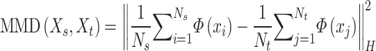The radial basis kernel function is used to calculate the MMD values of two probabilities distributions, and the smaller the MMD values, the more similar the two distributions are. In the KMM method, the inferred suitable is determined by solving the following minimization problem, and the objective function was given by the discrepancy between two empirical means and formulated as

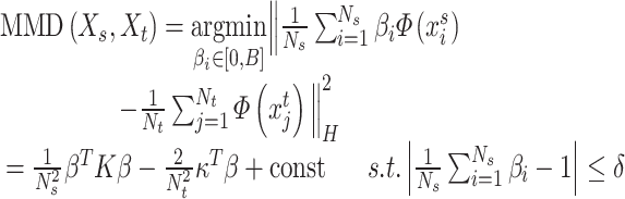where is the weighting parameter of each cell in scRNA-seq data and and are the corresponding expression of scRNA-seq and ST data, respectively. 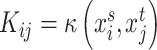is a kernel function, is a small parameter and B denotes a constraint parameter. Then, by extending and using kernel trick, the optimization problem can be transformed into a quadratic programming problem to find suitable . The computed and optimized probability density ratio can construct the relationship between the probability distribution of source domain and target domain. By using the data adjustment method, the target domain was adopted to assign weights to instances in the source domain; it can further reflect the importance of each instance according to the distribution similarity.

The probability density ratio of each cell was assigned to scRNA-seq data to match the distribution of scRNA-seq and ST data. In transfer learning, compared with the feature-based method, the instance-based transfer method can be used without changing the feature space of instances in source data. According to the weight generation rules, the instances in scRNA-seq data were reused, so that the weighted probability distribution of the source domain is similar to that of the target domain to the maximum extent. Through data adjustment, the representation space of scRNA-seq data remains and the adjusted scRNA-seq data still has good interpretability. Then, we can analyze the effect of distribution difference on the existing decomposition methods on raw and adjusted scRNA-seq data, respectively.

Datasets collection

The datasets in our study came from different sequencing techniques, protocols and platforms. The PDAC dataset has reliable regional marking information, and different regions are significantly divided. The diversity of cell types in the human heart dataset could be used to validate the performance of cell-type-specific genes in adjustment. The MOB dataset has an individual cell type per layer, which can characterize the spatial organization with layer structure. The detailed introduction and websites are provided in Supplementary Text 1 and Supplementary Table 1 available online at http://bib.oxfordjournals.org/.

Key Points

• Cell-type decomposition in ST data contributes to depicting the spatial organization of cell types.

• Distribution difference between scRNA-seq and ST data may result in bias in decomposition.

• Aiming to decrease the effect that some existing decomposition methods did not fully consider the difference and improve the decomposition results, we designed an instance-based transfer learning framework to match cell-type-specific gene expression by adjusting scRNA-seq data.

• In this framework, we evaluated the effect of raw and adjusted scRNA-seq data on cell-type decomposition by existing decomposition methods using simulated and real datasets.

• Experiments results showed that data adjustment reduced distribution difference and improved decomposition results. Further analyses indicated that the combination of data adjustment with decomposition methods can help to discover cell-type-specific genes, describe the spatial organization of cell types and reveal spatial heterogeneity.

Author Biographies

Lanying Wang is a PhD candidate of School of Computer Science and Technology at Xidian University. Her research interests include the development and improvement of computational methods on single-cell data analysis.

Yuxuan Hu is an Associate Professor of School of Computer Science and Technology at Xidian University. His research interests are in bioinformatics and cell communication.

Lin Gao is a Professor of School of Computer Science and Technology at Xidian University. She focuses on computational models and algorithms in analysis of single-cell data and omics-data.

FUNDING

This work was supported by the National Natural Science Foundation of China [62350087, 62132015 and U22A2037 to L.G., 62002277 to Y.H.].

DATA AVAILABILITY

The analysis code used to generate the figures and results is available at https://github.com/GaoLabXDU/STDecompositionAdjustment.

References

- 1. Marx V. Method of the Year 2020: spatially resolved transcriptomics. Nat Methods 2021;18:9–14. [DOI] [PubMed] [Google Scholar]
- 2. Zeng Z, Li Y, Li Y, Luo Y. Statistical and machine learning methods for spatially resolved transcriptomics data analysis. Genome Biol 2022;23(1):83. [DOI] [PMC free article] [PubMed] [Google Scholar]
- 3. Walker BL, Cang Z, Ren H, et al. Deciphering tissue structure and function using spatial transcriptomics. Commun Biol 2022;5(1):220. [DOI] [PMC free article] [PubMed] [Google Scholar]
- 4. Rao A, Barkley D, Franca GS, et al. Exploring tissue architecture using spatial transcriptomics. Nature 2021;596(7871):211–20. [DOI] [PMC free article] [PubMed] [Google Scholar]
- 5. Tian L, Chen F, Macosko EZ. The expanding vistas of spatial transcriptomics. Nat Biotechnol 2023;41(6):773–82. [DOI] [PMC free article] [PubMed] [Google Scholar]
- 6. Danaher P, Kim Y, Nelson B, et al. Advances in mixed cell deconvolution enable quantification of cell types in spatial transcriptomic data. Nat Commun 2022;13(1):385. [DOI] [PMC free article] [PubMed] [Google Scholar]
- 7. Li B, Zhang W, Guo C, et al. Benchmarking spatial and single-cell transcriptomics integration methods for transcript distribution prediction and cell type deconvolution. Nat Methods 2022;19(6):662–70. [DOI] [PubMed] [Google Scholar]
- 8. Ståhl PL, Salmén F, Vickovic S, et al. Visualization and analysis of gene expression in tissue sections by spatial transcriptomics. Science 2016;353(6294):78–82. [DOI] [PubMed] [Google Scholar]
- 9. Rodriques SG, Stickels RR, Goeva A, et al. Slide-seq: a scalable technology for measuring genome-wide expression at high spatial resolution. Science 2019;363(6434):1463–7. [DOI] [PMC free article] [PubMed] [Google Scholar]
- 10. Stickels RR, Murray E, Kumar P, et al. Highly sensitive spatial transcriptomics at near-cellular resolution with slide-seqV2. Nat Biotechnol 2021;39(3):313–9. [DOI] [PMC free article] [PubMed] [Google Scholar]
- 11. Liao J, Lu X, Shao X, et al. Uncovering an organ’s molecular architecture at single-cell resolution by spatially resolved transcriptomics. Trends Biotechnol 2021;39(1):43–58. [DOI] [PubMed] [Google Scholar]
- 12. Moses L, Pachter L. Museum of spatial transcriptomics. Nat Methods 2022;19(5):534–46. [DOI] [PubMed] [Google Scholar]
- 13. Palla G, Fischer DS, Regev A, Theis FJ. Spatial components of molecular tissue biology. Nat Biotechnol 2022;40(3):308–18. [DOI] [PubMed] [Google Scholar]
- 14. Chen J, Liu W, Luo T, et al. A comprehensive comparison on cell-type composition inference for spatial transcriptomics data. Brief Bioinform 2022;23(4):bbac245. [DOI] [PMC free article] [PubMed] [Google Scholar]
- 15. Liu B, Li Y, Zhang L. Analysis and visualization of spatial transcriptomic data. Front Genet 2022;12:785290. [DOI] [PMC free article] [PubMed] [Google Scholar]
- 16. Longo SK, Guo MG, Ji AL, Khavari PA. Integrating single-cell and spatial transcriptomics to elucidate intercellular tissue dynamics. Nat Rev Genet 2021;22(10):627–44. [DOI] [PMC free article] [PubMed] [Google Scholar]
- 17. Elosua-Bayes M, Nieto P, Mereu E, et al. SPOTlight: seeded NMF regression to deconvolute spatial transcriptomics spots with single-cell transcriptomes. Nucleic Acids Res 2021;49(9):e50. [DOI] [PMC free article] [PubMed] [Google Scholar]
- 18. Dong R, Yuan G-C. SpatialDWLS: accurate deconvolution of spatial transcriptomic data. Genome Biol 2021;22(1):145. [DOI] [PMC free article] [PubMed] [Google Scholar]
- 19. Ma Y, Zhou X. Spatially informed cell-type deconvolution for spatial transcriptomics. Nat Biotechnol 2022;40(9):1349–59. [DOI] [PMC free article] [PubMed] [Google Scholar]
- 20. Andersson A, Bergenstråhle J, Asp M, et al. Single-cell and spatial transcriptomics enables probabilistic inference of cell type topography. Commun Biol 2020;3(1):565. [DOI] [PMC free article] [PubMed] [Google Scholar]
- 21. Cable DM, Murray E, Zou LS, et al. Robust decomposition of cell type mixtures in spatial transcriptomics. Nat Biotechnol 2022;40(4):517–26. [DOI] [PMC free article] [PubMed] [Google Scholar]
- 22. Kleshchevnikov V, Shmatko A, Dann E, et al. Cell2location maps fine-grained cell types in spatial transcriptomics. Nat Biotechnol 2022;40(5):661–71. [DOI] [PubMed] [Google Scholar]
- 23. Sun D, Liu Z, Li T, et al. STRIDE: accurately decomposing and integrating spatial transcriptomics using single-cell RNA sequencing. Nucleic Acids Res 2022;50(7):e42. [DOI] [PMC free article] [PubMed] [Google Scholar]
- 24. Song Q, Su J. DSTG: deconvoluting spatial transcriptomics data through graph-based artificial intelligence. Brief Bioinform 2021;22(5):bbaa414. [DOI] [PMC free article] [PubMed] [Google Scholar]
- 25. Li H, Zhou J, Li Z, et al. A comprehensive benchmarking with practical guidelines for cellular deconvolution of spatial transcriptomics. Nat Commun 2023;14(1):1548. [DOI] [PMC free article] [PubMed] [Google Scholar]
- 26. Zhang Y, Lin X, Yao Z, et al. Deconvolution algorithms for inference of the cell-type composition of the spatial transcriptome. Comput Struct Biotechnol J 2022;21:176–84. [DOI] [PMC free article] [PubMed] [Google Scholar]
- 27. Sang-aram C, Browaeys R, Seurinck R, et al. Spotless: a reproducible pipeline for benchmarking cell type deconvolution in spatial transcriptomics. Elife 2023;12:n.p. [DOI] [PMC free article] [PubMed] [Google Scholar]
- 28. Maden SK, Kwon SH, Huuki-Myers LA, et al. Challenges and opportunities to computationally deconvolve heterogeneous tissue with varying cell sizes using single-cell RNA-sequencing datasets. Genome Biol 2023;24(1):288. [DOI] [PMC free article] [PubMed] [Google Scholar]
- 29. Jew B, Alvarez M, Rahmani E, et al. Accurate estimation of cell composition in bulk expression through robust integration of single-cell information. Nat Commun 2020;11(1):1971. [DOI] [PMC free article] [PubMed] [Google Scholar]
- 30. Avila Cobos F, Vandesompele J, Mestdagh P, de Preter K. Computational deconvolution of transcriptomics data from mixed cell populations. Bioinformatics 2018;34(11):1969–79. [DOI] [PubMed] [Google Scholar]
- 31. Schölkopf B, Platt J, Hofmann T. Correcting sample selection bias by unlabeled data. Adv Neural Inf Process Syst 2007;n.v.:601–8. [Google Scholar]
- 32. Eng C-HL, Lawson M, Zhu Q, et al. Transcriptome-scale super-resolved imaging in tissues by RNA seqFISH+. Nature 2019;568(7751):235–9. [DOI] [PMC free article] [PubMed] [Google Scholar]
- 33. Zeisel A, Manchado A, Codeluppi S, et al. Brain structure. Cell types in the mouse cortex and hippocampus revealed by single-cell RNA-seq. Science 2015;347(6226):1138–42. [DOI] [PubMed] [Google Scholar]
- 34. Chen A, Liao S, Cheng M, et al. Spatiotemporal transcriptomic atlas of mouse organogenesis using DNA nanoball-patterned arrays. Cell 2022;185(10):1777–1792.e21. [DOI] [PubMed] [Google Scholar]
- 35. Zeisel A, Hochgerner H, Lönnerberg P, et al. Molecular architecture of the mouse nervous system. Cell 2018;174(4):999–1014.e22. [DOI] [PMC free article] [PubMed] [Google Scholar]
- 36. Luecken MD, Theis FJ. Current best practices in single-cell RNA-seq analysis: a tutorial. Mol Syst Biol 2019;15(6):e8746. [DOI] [PMC free article] [PubMed] [Google Scholar]
- 37. Wang J, Huang M, Torre E, et al. Gene expression distribution deconvolution in single-cell RNA sequencing. Proc Natl Acad Sci U S A 2018;115(28):E6437–46. [DOI] [PMC free article] [PubMed] [Google Scholar]
- 38. Gretton A, Borgwardt KM, Rasch MJ, et al. A kernel two-sample test. J Mach Learn Res 2012;13:723–73. [Google Scholar]
- 39. Moncada R, Barkley D, Wagner F, et al. Integrating microarray-based spatial transcriptomics and single-cell RNA-seq reveals tissue architecture in pancreatic ductal adenocarcinomas. Nat Biotechnol 2020;38(3):333–42. [DOI] [PubMed] [Google Scholar]
- 40. Asp M, Giacomello S, Larsson L, et al. A spatiotemporal organ-wide gene expression and cell atlas of the developing human heart. Cell 2019;179(7):1647–1660.e19. [DOI] [PubMed] [Google Scholar]
- 41. Zhao E, Stone MR, Ren X, et al. Spatial transcriptomics at subspot resolution with BayesSpace. Nat Biotechnol 2021;39(11):1375–84. [DOI] [PMC free article] [PubMed] [Google Scholar]
- 42. Tepe B, Hill MC, Pekarek BT, et al. Single-cell RNA-seq of mouse olfactory bulb reveals cellular heterogeneity and activity-dependent molecular census of adult-born neurons. Cell Rep 2018;25(10):2689–2703.e3. [DOI] [PMC free article] [PubMed] [Google Scholar]
- 43. Hosna A, Merry E, Gyalmo J, et al. Transfer learning: a friendly introduction. J Big Data 2022;9(1):102. [DOI] [PMC free article] [PubMed] [Google Scholar]
- 44. Qian C, Zhu J, Shen Y, et al. Deep transfer learning in mechanical intelligent fault diagnosis: application and challenge. Neural Process Lett 2022;54(3):2509–31. [Google Scholar]
- 45. Bai J, Jia J, Capretz LF. A three-stage transfer learning framework for multi-source cross-project software defect prediction. Inf Softw Technol 2022;150:106985. [Google Scholar]
- 46. Hu J, Li X, Hu G, et al. Iterative transfer learning with neural network for clustering and cell type classification in single-cell RNA-seq analysis. Nat Mach Intell 2020;2(10):607–18. [DOI] [PMC free article] [PubMed] [Google Scholar]
- 47. Wang YM, Sun Y, Wang B, et al. Transfer learning for clustering single-cell RNA-seq data crossing-species and batch, case on uterine fibroids. Brief Bioinform 2023;25(1):bbad426. [DOI] [PMC free article] [PubMed] [Google Scholar]
- 48. Shen R, Liu L, Wu Z, et al. Spatial-ID: a cell typing method for spatially resolved transcriptomics via transfer learning and spatial embedding. Nat Commun 2022;13(1):7640. [DOI] [PMC free article] [PubMed] [Google Scholar]
- 49. Halawani R, Buchert M, Chen YP. Deep learning exploration of single-cell and spatially resolved cancer transcriptomics to unravel tumour heterogeneity. Comput Biol Med 2023;164:107274. [DOI] [PubMed] [Google Scholar]
- 50. Li H, Wang Z, Lan C, et al. A novel dynamic multiobjective optimization algorithm with non-inductive transfer learning based on multi-strategy adaptive selection. IEEE Trans Neural Netw Learn Syst 2023;PP:1–15. [DOI] [PubMed] [Google Scholar]
- 51. Zhuang F, Qi Z, Duan K, et al. A comprehensive survey on transfer learning. Proc IEEE Inst Electr Electron Eng 2021;109(1):43–76. [Google Scholar]
- 52. Iman M, Arabnia HR, Rasheed K. A review of deep transfer learning and recent advancements. Dent Tech 2023;11(2):40. [Google Scholar]
- 53. Mao L, Wang L, Hu LS, et al. Weakly-supervised transfer learning with application in precision medicine. IEEE Trans Autom Sci Eng 2023;n.v.:1–15. [Google Scholar]
Associated Data
This section collects any data citations, data availability statements, or supplementary materials included in this article.
Supplementary Materials
Data Availability Statement