

Abstract
Ctfplotter in the IMOD software package is a flexible program for determination of CTF parameters in tilt series images. It uses a novel approach to find astigmatism by measuring defocus in one-dimensional power spectra rotationally averaged over a series of restricted angular ranges. Comparisons with Ctffind, Gctf, and Warp show that Ctfplotter’s estimated astigmatism is generally more reliable than that found by these programs that fit CTF parameters to two-dimensional power spectra, especially at higher tilt angles. In addition to that intrinsic advantage, Ctfplotter can reduce the variability in astigmatism estimates further by summing results over multiple tilt angles (typically 5), while still finding defocus for each individual image. Its fitting strategy also produces better phase estimates. The program now includes features for tuning the sampling of the power spectrum so that it is well-represented for analysis, and for determining an appropriate fitting range that can vary with tilt angle. It can thus be used automatically in a variety of situations, not just for fitting tilt series, and has been integrated into the SerialEM acquisition software for real-time determination of focus and astigmatism.
Keywords: Electron cryo-tomography, contrast transfer function, CTF, astigmatism
Graphical Abstract

1. Introduction
Cryo-electron tomography (cryoET) with subtomogram averaging has proved to be a powerful method for determining molecular structures at high resolution. Accurate determination of and correction for the effects of the microscope contrast transfer function (CTF) is important for preserving the high-resolution information in this process. Two factors make CTF determination difficult for tilt series images: the variation in defocus across images taken away from zero tilt; and the low signal-to-noise ratio (SNR) of each image compared to that of typical images for single-particle reconstruction. The first factor is addressed by analyzing data in strips parallel to the tilt axis (Fernandez et al., 2006; Xiong et al., 2009; Chen et al., 2019). Low SNR was originally overcome by summing signal from multiple images when necessary (Fernandez et al., 2006; Xiong et al., 2009). It has become less of a problem due to two factors: the availability of efficient cameras with direct electron detection and electron counting; and the use of high tilt increments (typically 3°) that allow doses of 2–3 e/Å2 per image (e.g., (Schur et al., 2016)). Defocus can now be estimated accurately in single images for many cryo-tilt series.
Determination of astigmatism remains problematic even with 2–3 e/Å2 images. The usual approach is to search for defocus and the two parameters of astigmatism simultaneously by fitting to a two-dimensional (2-D) power spectrum after first obtaining an estimate of defocus from rotationally averaged (1-D) power spectrum. This approach is used in Ctffind (Rohou and Grigorieff, 2015) and Gctf (Zhang, 2016), which are free-standing programs commonly used for CTF fitting; e.g., RELION (Kimanius et al., 2021) allows fitting with either. Ctfplotter uses a different, novel approach to finding astigmatism: defocus is measured in a series of 1-D spectra rotationally averaged over sectors of the 2-D spectrum, referred to as wedges, and the underlying astigmatism is found by fitting to these defocus values. Sectors of power spectra have been used before in goCTF (Su, 2019), but only to improve SNR by selecting the subset of a spectrum with the most signal. It is shown here that good estimates can be obtained from relatively wide wedges (90°), and thus the SNR for these measurements is not greatly reduced from the SNR when fitting to a whole 1-D spectrum.
The performance of Ctfplotter was evaluated on test images and tilt series and compared with that of Ctffind, Gctf, and Warp (Tegunov and Cramer, 2019), which uses a more sophisticated approach to CTF fitting than the two free-standing programs. The test images were generated from 500-frame stacks obtained by long exposures of stable specimens, and the dependence of the CTF fitting on SNR was explored by summing different numbers of frames. The results from these tests and from tilt series will show that the wedge method gives more reliable estimates of astigmatism when SNR is low than the programs using 2-D fitting. Ctfplotter also determines phase shift in tilt series more reliably than the other programs. This paper also describes other developments that have made the program more accurate and easier to use, to the point where it can now be run automatically on a variety of data with the entry of relatively few parameters.
2. Methods and results
2.1. Baseline fitting to replace noise spectra
Ctfplotter was originally written when images were acquired on CCD cameras with poor response at higher spatial frequencies, giving power spectra with a relatively weak CTF signal imposed on a curve that declined strongly with frequency. Instead of attempting to find a baseline to subtract, it required a set of blank images, collected once for a camera and microscope, to provide noise spectra that were divided into the measured power spectra (Xiong et al., 2009). With the advent of direct electron detection, and especially electron counting, CTF signals became stronger and spectra did not decline so much with frequency, so it became feasible to fit a baseline instead of using noise spectra. The program does this in two stages. First it searches for a ”break point” in the spectrum, a frequency at which the angle between a line fit before that point and line fit after it is largest (Fig. 1A), similar to an approach used in CTER (Penczek et al., 2014). Then, it smooths the spectrum past that point with a Gaussian kernel small enough to preserve CTF oscillations and finds local minima at spacings appropriate for being zeros if possible, or falls back to picking points at a minimum interval of 3 if not (Fig 1B, see legend for details). This subset of points is fit with a polynomial that is constrained to be concave upward or downward (i.e., the second derivative is not allowed to have zeroes over the fitting range, which makes the first derivative change monotonically). The polynomial order can be selected from 1 to 4, but 4 is the default because the constraint prevents the inflections that higher order polynomials are prone to.
Figure 1.

Fitting a baseline for background subtraction. A. In the first stage of the operation, two lines are fit to the power spectrum at a series of potential break points around the expected location of the first zero. The fit at lower frequency includes the candidate break point and 3 points to the left (solid lines); the other fit includes that point and all but 3 points out to Nyquist (dashed lines, longer dashes). For this particular example, the lowest point evaluated has an angle between the lines of 56° (red lines); the last point where the left line has a negative slope gives an angle of 47° (blue lines). The optimal break point is chosen as the one that gives the highest angle, 89° (green lines). The high-frequency line is extended to the left to provide the initial baseline (green short dashes). B. In the second stage, this baseline is subtracted and the spectrum is smoothed with a Gaussian whose sigma is 0.1 times the expected spacing between first and second zeros, but constrained to be between 1 and 2.5. Minima are found in this smoothed spectrum, plus points at regular intervals where no minima occur (red circles). A polynomial with no inflections, of order up to 4, is fit to these points and linearly extrapolated past the first and last points (green curve). The resulting curve is added to the initial baseline to obtain the final baseline. This spectrum is from the 3 lowest tilt views of TS_03 from the EMPIAR-10164 deposition.
The baseline-subtracted 1-D spectrum is fit with a simplex search (Lagarius et al., 1998) to a curve based on a standard CTF function:
| (1) |
where is frequency, is electron wavelength, is spherical aberration, is defocus, is phase, and is amplitude contrast. The function fit is:
| (2) |
where the variables searched are defocus, , , , , , and possibly the exponent , which is generally fixed at 1.5 but can be varied to fit the actual shape of the spectrum better. The two exponentials allow separate fitting of the steeply falling part of the curve before the first zero and the decay of the spectrum thereafter.
2.2. Finding astigmatism
The first attempt to implement astigmatism determination in IMOD involved adapting Ctffind (Rohou and Grigorieff, 2015) into a library that could be incorporated into Ctfplotter to fit directly to 2-D power spectra, the conventional approach. The results were not satisfactory, especially with higher-tilt images, and this approach was abandoned in favor of the one described next. However, the library is still in IMOD, can be used with a program called Testctffind, and allowed CTF fitting to be done in SerialEM (Mastronarde, 2005), after optimizations to provide real-time fits in reasonable time.
Ctfplotter finds astigmatism by measuring defocus in spectra extracted from limited angular ranges, i.e., wedges in the 2-D power spectrum. Figure 2A depicts two 90° wedges oriented along the long and short axes of astigmatism in a power spectrum. The 1-D spectra computed from each wedge have clearly different zero positions reflecting their different defoci (Fig. 2B). These raw measurements, however, do not indicate the full range of defocus. The defocus values for a full range of wedge angles are plotted in Fig. 3 for both these 90° wedges and for 10° wedges, which give good defocus estimates in this case because of the high SNR of the image. The 90° wedges give a lower range of defocus because orientations with the most extreme defocus are averaged with less extreme ones. To derive astigmatism from any wedge size, the program finds the defocus values and , and axis angle that makes the expected average defocus values for the wedges fit the measured values. The average defocus for a wedge with angular range and center angle is obtained by integrating the formula for defocus at angle :
| (3) |
and is
| (4) |
Robust fitting is used to reduce the effects of outlying defocus measurements. If the astigmatism estimate implies that defocus varies enough within the wedge to blur out the highest frequency oscillations within the fitting range, the procedure is iterated. This time, the wedge is divided into non-overlapping subranges within which defocus varies by less than an amount that would blur out oscillations; Fig. 2D shows these subranges for the wedge at 25°. The 1-D spectrum for each subrange is adjusted by the difference between its expected defocus and the expected average defocus of the wedge. These adjusted spectra are summed to get a wedge spectrum that preserves the higher frequency zeros (Fig 2C). Iterations continue until the change in astigmatism is sufficiently small. For the example in Figs. 2–3, 90° wedges gave an initial estimate of 0.493 μm, whereas iterating with the subranges gave values of 0.438 and 0.440 μm, in good agreement with the estimate of 0.439 μm with 10° wedges. With this final value of astigmatism and a good estimate of average defocus, the program computes a full spectrum by summing spectra from angular subranges adjusted to match that average defocus. This spectrum is fit to obtain the final defocus value.
Figure 2.
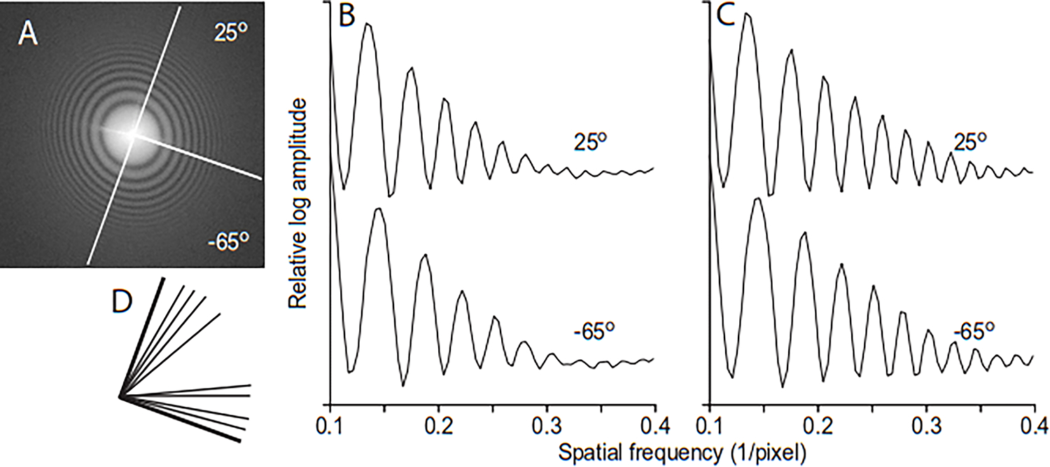
Example of measuring astigmatism with 1-D power spectra from 90° wedges of the 2-D power spectrum. The sample was a 2000 lines/mm carbon replica cross-line grating with a Au/Pd coating, imaged on a K3 camera at 200 kV with a pixel size of 0.182 nm, 65 electrons recorded per pixel, and dose over 25 e/Å2. The image was taken at 2μm underfocus with an astigmatism of ~0.4 μm imposed. A. Power spectrum of image, with lines showing two 90° wedges along the short and long axes of astigmatism. B. 1-D spectra summed from the 90° angular ranges depicted in A; these partial spectra have good signal-to-noise ratio and reflect the difference in defocus on the two axes. C. 1-D spectra from the second iteration of finding astigmatism, in which angular subranges are adjusted for their expected differences in defocus before summing; the sums preserve the high-frequency information better. D. Non-overlapping angular subranges selected by Ctfplotter to keep the defocus variation within each subrange under a criterion amount.
Figure 3.

Variation in defocus in 1-D spectra measured with 10° and 90° wedges from the example in Fig. 2. The values need to be fit to a model to estimate the underlying astigmatism.
Iterating with defocus-adjusted subranges not only allows a more accurate fit but also reduces bias from orientation-dependent signal strength. Suppose signal is weak along the long axis of astigmatism. For 90° wedges oriented near that axis, the spectrum will be dominated by the stronger signal at other angles and the measured defocus will be too low, leading to an underestimate of astigmatism. On iterating, the subranges are adjusted to match the defocus expected for the wedge given this astigmatism, and the defocus measured for the wedge increases because the spectrum is dominated by signals adjusted to a higher defocus. Iterations can thus converge on a more correct value of astigmatism.
The program uses 90° wedges by default so that the SNR will be only half that of a full spectrum; it is thus important to establish that astigmatism estimates are not biased by using such large wedges. Figure 4A shows that the estimate is essentially constant with wedge range for the high-dose example in Figs. 2 and 3. The dependence of astigmatism on wedge range was examined for nine tilt series with astigmatism ranging from 0.02 to 0.22 μm. For each wedge range, the difference from the estimate with 90° wedges was averaged over all of the tilts, or ones with the highest astigmatism. Figures 4B–F show these averaged differences for the five tilt series with astigmatism above 0.06 μm. No consistent trend is seen in such graphs. If anything, the trend is for smaller wedges to give slightly smaller estimates, but the differences are all under 10 nm. Thus, astigmatism can be estimated accurately with 90° wedges.
Figure 4.

Dependence of astigmatism estimate on size of wedges, expressed as the difference between the estimate at a given wedge size and that with 90° wedges, in nanometers. A. Results from the example image in Fig. 2. B-F. Values averaged over most or all tilt angles in a tilt series, for 5 tilt series with astigmatism above 0.06 μm. The dependence on wedge size is small and not in a consistent direction for different tilt series.
2.3. Comparisons based on frame sums
To compare CTF results with those from other programs and assess the effects of noise on fitting performance, 500-frame stacks were acquired from Gatan K2 or K3 cameras and analyzed by varying the number of frames summed per image. Untilted images were taken of the carbon film in a grid used for cryoEM and of a 2160 lines per mm cross-line grating, at a variety of astigmatism values, with a pixel size of ~2.3 Å and ~0.6 electrons per frame. Sequential sets of frames were aligned and summed with Alignframes in IMOD, ranging from 100 sums of two frames each to five sums of 100 frames each. The summed images were processed with Ctfplotter, Gctf, Ctffind, and Warp, and statistics were computed for each amount of summing. Comparisons with Gctf and Ctffind are shown in Fig. 5. Because the images with different astigmatism values showed similar patterns of results, the results presented in Fig. 5 are based on averages over all four or five images for each specimen. To average astigmatism values, each value was expressed relative to the astigmatism found by Ctfplotter from 100-frame sums of the respective frame set. The error bars in Figs. 5B and E are one standard error of the mean and provide a rough guide for which differences are statistically significant (i.e., ones where the bars do not overlap). The existence of significant differences between curves indicates that this is a useful way to summarize the trends. Note that Ctffind 4.1.8 was used for these and other comparisons reported here; Ctffind 4.1.9 to 4.1.14 perform considerably worse at lower doses (corresponding to < 25 summed frames in these graphs). This problem was caused by a masking step that attenuates low frequencies too much for noisier spectra; the step can be skipped with an option in Testctffind and a similar option should appear in a newer version of Ctffind.
Figure 5.

Comparison of performance of Ctfplotter, Ctffind, and Gctf with images at a range of doses generated by composing aligned sums of different sizes from 500-frame exposures. A-C are based on images taken with a Gatan K3 camera on a Thermo Fisher Talos Arctica microscope operating at 200 kV. The specimen was a quantifoil grid after a cryoEM session; the area was stabilized with extensive exposure before the images were taken. The pixel size was 0.222 nm; 0.56 electrons were recorded per frame, for a dose at the camera of ~0.11 e/Å2 per frame. Results are averaged from four images with astigmatisms of 0.22, 0.4, 0.63, and 0.85 μm. D-F are based on images taken with a Gatan K2 camera on a Thermo Fisher F30 microscope operating at 300 kV. The sample was a 2160 lines/mm carbon replica cross-line grating. The pixel size was 0.257 nm; 0.63 electrons were recorded per frame, for a dose at the camera of ~0.09 e/Å2 per frame. Results are averaged from five images with astigmatisms of 0.13, 0.28,0.46,0.65, and 0.84 μm. A, D. Behavior of defocus for different sized sums. B, E. Behavior of astigmatism. For each frame series, the astigmatism found by Ctfplotter with 100-frame sums was subtracted from the average astigmatism for each frame sum; means and SDs were computed from these differences. The error bars are one standard error of the mean. For the carbon film (B), Gctf error bars are omitted for clarity; they were almost twice as big as those of Ctffind on average. C, F. Standard deviation of astigmatism estimates for different sized sums, showing better performance of the wedge method in Ctfplotter. The four or five separate values of SD, respectively, were averaged for each point in the graphs.
Three aspects of these graphs are to be considered:
Consistency among programs: The values at the right in each graph are from high-dose images and are thus the best estimates from each program. Defocus is ~10 nm higher for Ctffind than Ctfplotter for both specimens; for Gctf, the difference is even greater with the carbon film but about the same with the cross-line grating (Figs. 5A, D). Astigmatism is nearly the same for Ctfplotter and Ctffind with the carbon film (Fig. 5B), but ~10 nm less for Ctfplotter with the cross-line grating (Fig. 5E). Such differences do not occur with simulated images, so they presumably reflect how the programs behave differently with non-ideal images.
Dependence on dose: For the carbon film, both the defocus and astigmatism found by Ctfplotter are close to constant with decreasing dose (Figs. 5A, B). The same is true for Ctffind except at the lowest few doses. Gctf shows much less consistency in both defocus and astigmatism as dose is lowered into the range for tilt series images. For the cross-line grating images, all three programs show changes in defocus as the dose is reduced, ~10 nm for Ctfplotter and Ctffind, and more for Gctf (Fig 5D). The astigmatism estimate for Ctfplotter drops by 10 nm at lower doses (Fig. 5E). Again, the changes in these graphs probably reflect the different responses to this particular non-ideal specimen, with its mixture of carbon and gold crystal.
Variability of results: Ctfplotter has the lowest variability for both specimens, as assessed by the mean standard deviation (SD) of measurements (Figs. 5C, F). Note the logarithmic scale to encompass the wide range of variability. The near-constant spacing between curves indicates that Ctfplotter gives 1.5–2 times lower variability at all but the highest dose. Gctf does worse with the carbon film and Ctffind does worse with the cross-line grating. The same patterns occur in graphs of the SD not just for the astigmatism axis angle but also for defocus at all but the highest dose. The wedge method gives an intrinsically more accurate astigmatism value, and fitting to a 1-D spectrum with astigmatism taken into account then gives a less variable result for defocus than is obtained by fitting all parameters at once to the 2-D spectrum.
Comparisons with Warp are more ambiguous (Fig. 6). Overall, Warp gave higher variability in astigmatism estimates for the carbon film, except at a range of lower doses (Fig 6A). With the cross-line grating, it did markedly worse for all doses using the default amplitude contrast of 0.07; fitting improved either with higher amplitude contrast or with phase included in the solution. The best results, with an amplitude contrast of 0.14, are consistently worse than those from Ctfplotter with its default amplitude contrast of 0.07 (Fig. 6B). Variability from Ctfplotter with amplitude contrast 0.14 was generally higher, matching that of Warp over a range of lower doses as in Fig. 6A (results not shown). In this case, the overall averages conceal the fact that, at the lowest astigmatism, Warp did consistently better than Ctfplotter for the carbon film and matched it for the cross-line grating.
Figure 6.

Comparison of the performance of Warp and Ctfplotter for the sets of summed frames used in Figure 5. A. SD of astigmatism averaged over the 4 sets from carbon film. Warp does worse except for a range of lower doses. B. SD of astigmatism averaged over the five sets from cross-line replica grating. Warp with amplitude contrast at 0.14 (crosses) did consistently worse than Ctfplotter with the default setting of 0.07 (circles).
2.4. Comparisons for cryo-tilt series
Results from cryo-tilt series are consistent with these findings, if greater tilt-to-tilt variability is considered to reflect less accurate values. Figure 7 shows values of defocus and astigmatism for tilt series TS_03 of the EMPIAR-10164 deposition (Schur et al., 2016), chosen because of the large amount of astigmatism that developed at negative tilt angles. For both Ctffind (Fig. 7A) and Gctf (Fig. 7B), the greater variability for defocus is most apparent at positive tilt angles where defocus is nearly constant. The astigmatism values show both greater variability and simply inaccurate values above +40° (note the logarithmic scale in Figs. 7C and D). Warp did better than these two programs and showed visibly worse variability only at higher tilts (data not shown).
Figure 7.
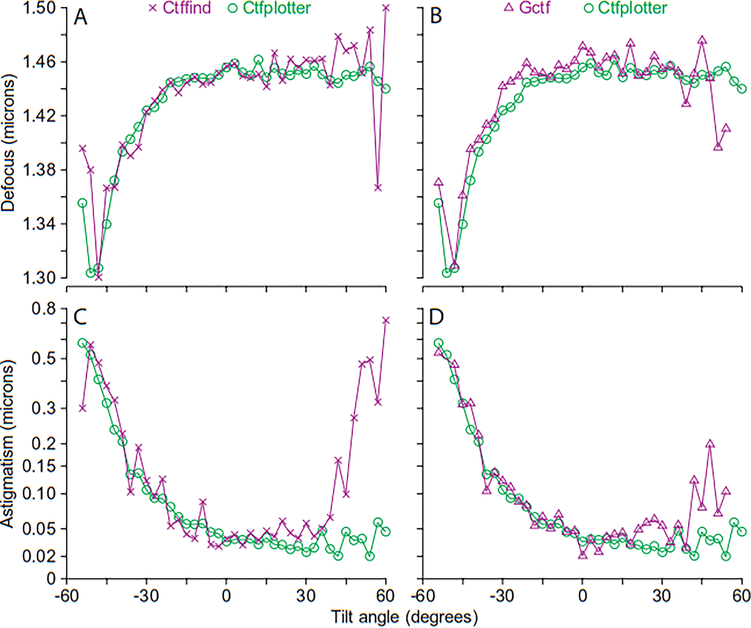
Performance of Ctfplotter, Ctffind, and Gctf on a cryo-tilt series with strong CTF signal and substantial astigmatism. The tilt series of HIV virus-like particles is TS_03 from the EMPIAR-10164 deposition, with a pixel size of 0.135 nm and dose of 2.4 e/Å2 per image, which resulted in ~1.4 electrons recorded per pixel. The raw frames were aligned with Alignframes by John Heumann. A, B. Defocus found by Ctfplotter and Ctffind (in A) or Gctf (in B). Ctfplotter has less tilt-to-tilt variability. C, D. Astigmatism found by Ctfplotter and Ctffind (in C) or Gctf (in D). Ctfplotter does much better at positive high tilts.
Ctfplotter has an additional way to improve astigmatism accuracy for tilt series with less robust results than in Fig. 7: summing spectra from multiple consecutive tilt angles. Such summing is appropriate for astigmatism because it is an optical parameter that would be expected to change slowly and continuously during a tilt series. Figure 8 shows results from a tilt series of Borrelia burgdorferi with empty ice in half of the field; with fitting to single images, Ctfplotter gave a fair amount of tilt-to-tilt variability in both astigmatism amount and axis angle, but Warp gave much worse variability for each at higher tilt (Fig. 8A, B). Much more consistent values were obtained by summing from five images at each angle (Fig. 8C, D). After getting this improved astigmatism estimate at an angle, the program drops back to a single image for measuring defocus. Because of results like these, the default setting in Ctfplotter is to measure astigmatism from five images in this way.
Figure 8.

Astigmatism estimates from Ctfplotter and Warp and benefits of estimating astigmatism from summed images for a cryo-tilt series with weaker CTF signal. This tilt series of Borrelia burgdorferi was provided by Yunjie Chang and Jun Liu, taken with a Gatan K2 camera on a Thermo Fisher Krios operating at 300 kV, with a dose of ~2 e/Å2 per image. With this tilt series, Ctfplotter was run with super-resolution images, but other programs were run with images reduced by 2 because Gctf and Ctffind performed poorly otherwise. Ctfplotter did equally well with reduced images. A, B. Magnitude of astigmatism (A) and angle of astigmatism axis (B) when Ctfplotter measured astigmatism with single images. Warp did much worse except near zero tilt. C, D. Astigmatism magnitude and axis angle when Ctfplotter used sums of five images to find astigmatism. The summing reduced the implausible tilt-to-tilt variability.
To quantify the astigmatism variability in tilt series, a deviation was computed between the estimated astigmatism at each tilt angle and the value at that angle of a parabola fit to the nearest 9 points. The five tilt series of EMPIAR 10164 were processed in Warp, using either the tilt images from Alignframes as in Fig. 7, or the original super-resolution frames. The results are in Table 1. The mean deviation averaged over the five tilt series and the median of maximum deviations both showed a similar pattern: astigmatism found from one image in Ctplotter had half as much variability as with Warp, and the variability was lower by another half when summing over five images. (In the latter case, each deviation was measured from a parabola fit to the values found with one image, because the values found with five images are not independent between tilts). When only the lower tilt images are considered (+/−30°), Warp does as well as Ctfplotter with one image, but again summing over five images is twice as good. For the challenging Borrelia set in Fig. 8, Warp, Ctffind, and Gctf gave similar results and Ctfplotter did much better overall. The other programs did better with lower tilt images but Ctfplotter using five images still gave a much better result.
Table 1.
Variability of astigmatism estimates in tilt series
| EMPIAR-10164 | Borrelia | ||||
|---|---|---|---|---|---|
| Mean of mean deviations | Median of maximum deviations | +/−30° mean deviation | Mean deviation | +/−30° mean deviation | |
|
| |||||
| Warp from frames | 19.1 | 57 | 14.9 | ||
| Warp from images | 13.8 | 49 | 5.3 | 49 | 25 |
| Ctfplotter from 1 image | 7.9 | 27 | 5.6 | 18 | 19 |
| Ctfplotter from 5 images | 3.8 | 15 | 2.5 | 8 | 8 |
| Ctffind | 45 | 32 | |||
| Gctf | 42 | 20 | |||
Assessment of astigmatism variability in tilt series from the deviations between individual values and parabolas fit to 9 values; see text for details. Values are in nanometers. Mean deviations are averaged over entire tilt series or over images between +/−30° of tilt.
2.5. Finding Phase Shift
Phase shift from a phase plate changes the CTF zero positions in a defocused image in a characteristic way, so in principle phase can be found as an additional parameter when fitting to the spectrum. However, in Ctfplotter the fit to the 1-D spectrum already involves searching for four or five parameters in addition to defocus (Eq. 2), and including phase as an additional parameter in this fit gave unreliable results, probably because defocus and phase can covary to produce nearly equivalent fits. The solution was to do an outer 1-D search for the phase that gives the best fit to the spectrum in the usual search for defocus and the other parameters. This search can be done on a spectrum summed from adjacent tilts; after phase is found from the less noisy spectrum, the defocus can be found for a single image with that phase value. A small inaccuracy in the phase from assuming that it is constant will be compensated by a defocus value that makes the spectrum fit adequately.
Unfortunately, the standard model for a fixed phase effect may not fit the actual zero positions well; the model may require a soft cut-on for the effect (Danev et al., 2017). Figure 9A shows the actual and fitted curves for a tilt series of Schizosaccharomyces pombe taken with a Volta phase plate, provided by Julia Mahamid and Sara Goetz, and similar to data available in EMPIAR-10988 (de Teresa-Trueba et al., 2023). The top curves are from fitting to the spectrum itself, which is dominated by the larger amplitudes at the lower frequencies; the curves fit poorly at the highest frequencies. The bottom curves are from an alternative method developed to alleviate this problem, in which the program finds the zeros in the 1-D spectrum, then finds the defocus and phase that best fit those zero locations. Here the fit is reasonably good at the higher frequencies but visibly off for the second through fourth ones. To add a soft cut-on, phase is modeled as rising exponentially from zero to its value at infinity. To provide more stable phase values, the parameter searched for is the phase at 0.3/nm, , and the phase at frequency is
| (5) |
where is the cut-on frequency in 1/nm. With a cut-on frequency included, the computed curve fits the zeros better throughout the frequency range, regardless of whether the spectrum or the zero positions are fit (Fig. 9B). The square of the ratio in the exponential was tried, as in Eq. 1 of (Danev et al., 2017), but this usually gave higher errors in fitting to zero positions, ~22% higher on average for the two tilt series used in Fig. 9.
Figure 9.

Estimation of phase shift and the results of incorporating a soft cut-on in the phase shift. A. Fits to spectrum computed from three lowest-tilt images of tilt series from Julia Mahamid and Sara Goetz taken with a Volta phase plate. The sample was a platinum-coated cryo-FIB lamella of Schizosaccharomyces pombe and images were taken on a Krios at 300 kV with a K2 camera at a nominal defocus of 3 μm. With phase included in the fit, the regular fit between the spectrum (magenta) and CTF-like curve (green) gets off at high frequency (upper curves, arrow to right); a fit using zero positions gets of most visibly at lower frequencies (lower curves, arrow to left). B. Better-fitting curves obtained with a cut-on frequency included in the fit. C. Defocus found by Ctfplotter and Gctf from a similar tilt series, TS_0001 of EMPIAR-10988. Gctf fits for C and D were done with parameters optimized by Rado Danev on the tilt series in A and B. Gctf gets off at high tilt. D. Phase found by Gctf and by Ctfplotter with fitting to spectrum or to zero positions. E. Cut-on frequencies found with fitting to spectrum or to zero positions.
Finding a cut-on frequency is difficult because the error of the CTF fit with the best phase value for a particular cut-on frequency varies quite slowly with cut-on frequency (supplemental Figure S1). Rather than doing a 2-D search for phase and cut-on, the program does nested 1-D searches. The outer search is on cut-on frequency, starting with a scan over a wide range, then refining from the global minimum. At each cut-on frequency evaluated, a 1-D search is done for the best phase, as described above. If the outer search fails to find a minimum, the program picks a fallback value from nearby tilt angles, if possible, and proceeds to find phase and defocus with that value.
Results from fitting phase and cut-on frequency for one of the tilt series in EMPIAR-10988 are shown in Figs. 9C–E, along with defocus and phase values from Gctf. Phase increases in both directions from 0° because the tilt series was taken with a dose-symmetric scheme (Hagen et al., 2017). Phase and cut-on were found in spectra summed from three tilt angles. The tilt-to-tilt variability of cut-on is considerable even with that summing, and there is roughly a 35% difference between cut-on values found by the two different fitting methods (Fig. 9E). Both of these facts reflect the insensitivity of the fit to the actual cut-on frequency. Nevertheless, the phase shifts vary smoothly, with ~5° difference in the values found with the two fitting methods (Fig. 9D). This difference in phase is in turn accommodated by a ~15 nm difference in defocus (not shown). Although the underlying true value of these parameters is elusive, the goal of locating the zeros for CTF correction is achieved. Gctf gave a 20° higher phase value at the low tilts; it did find most of the phase increase in the lower tilts of the series but did poorly on both phase and defocus at higher tilts (Figs. 9C, D). Ctffind did no better (not shown); it found a phase of 85° for the lowest tilts but did not track the phase increase nearly as well as Gctf. The advantages of using Ctfplotter to find phase in tilt series are evident.
2.6. Features for improved fitting on high-resolution tilt series
When Ctfplotter is run with its default parameters on high-resolution cryo tilt series, it will generally give a spectrum that does not show the CTF signal well because it is not sampled finely enough (i.e., CTF aliasing). (By default, the 1-D spectrum is computed with only 101 points in order to maintain a good SNR with weaker signals.) There are two mechanisms for avoiding this effect: 1) extracting tiles larger than the specified size (256 × 256 by default) and cropping their Fourier transforms before computing the power spectrum, effectively increasing the pixel size of the data; 2) increasing the number of points in the 1-D spectrum. When the program is run interactively, it displays messages indicating whether the spectrum is undersampled within the range of frequencies being fit and suggests how to change the cropping and/or the number of points to achieve at least 3.5 sample points between zeros. The first method is preferred because it spreads out the usable signal to fill the graph area, but once that is the case, the number of points needs to be increased. Adjusting the sampling usually takes at least two iterations because the initial change reveals usable signal past the end of the fitting range, and when that range is increased, the program suggests a new change in sampling.
Three features were developed with two goals: to reduce the effort involved in adjusting this sampling and in revising the fitting range for different parts of the tilt range; and to improve the convenience and reliability of completely automated fitting. First, because the spectrum fitting relies on having a fairly accurate value for the expected defocus, there is an option to try fitting with a range of expected defocus values on startup. A subset of that range will result in the same defocus value, and that is taken as the expected defocus for further fitting. This feature is particularly useful when doing batch processing of a set of tilt series taken with a range of defocus values. Second, the program can “autotune” the spectrum sampling and the fitting range by iteratively making the changes suggested in the dialog when running interactively, and by using the local correlation between the spectrum and fitted CTF curve to determine the end of the fitting range at each step. Third, fitting can be done with weighting of the errors by a function of this local correlation, which will automatically truncate the effective fitting range when high-frequency signal gets weaker at higher tilt angles. With this feature, there is no need to adjust the fitting range manually when fitting automatically to the entire series.
Figure 10 illustrates these features with tilt series TS_01 of EMPIAR-10164, which is an extreme case of bad initial sampling with the default number of frequency points (101), because of the 4 μm defocus combined with a 0.135 nm pixel size. Ctfplotter was started with the option to try a defocus range of 1 to 8 μm and it found a defocus of 3.9 μm (Fig. 10A). In this defocus scan, and for the autotuning, it crops spectra to a pixel size of 0.27 nm if the pixel size is smaller; it can thus work with much better spectra than the CTF-aliased one in Fig 10A, making the fitting more reliable. After the “Autotune” button was pressed, the program settled on cropping to 0.26 nm and computing 173-point power spectra, and it adjusted the vertical scaling based on the amplitude after the first zero (Fig. 10B; note that the periodicity at the right end of the graph has changed from 2.7 Å to 5.2 Å to reflect the cropping). It set the fitting range as indicated by the extent of the blue curve, which plots the weighting being applied based on the local correlation with the CTF curve. Three images were summed for the defocus scan and tuning. Automatic fitting to single images over the whole tilt series could then be done with these settings; the blue curve in Fig. 10C shows how the fitting range was appropriately truncated for the image at −57°.
Figure 10.

Example of autotuning and automatic truncation of fitting range, using tilt series TS_01 of EMPIAR-10164. A. Ctfplotter window when the program is first started, showing the baseline-subtracted spectrum of the three lowest-tilt images in magenta and the fitted curve in green. The X axis labels are frequency in reciprocal pixels and periodicity in Angstroms. The Y axis is the baseline-subtracted logarithm of the spectrum amplitude. B. After autotuning, the tuned spectrum sampling retains high-frequency oscillations; the cyan curve shows the weights applied when fitting the two curves, based on their local cross-correlation. C. Curves from fit to single image at −57°.
2.7. Program Speed Enhancements
With these three features available, Ctfplotter can now be used non-interactively to find CTF reliably with about the same degree of parameter entry as for Ctffind and Gctf. It thus became feasible to run Ctfplotter from SerialEM instead of using the built-in CTF fitting available with the Ctffind-based library from IMOD. Using Ctfplotter gives intrinsically better astigmatism estimates for zero-tilt images (Fig. 5), plus reliable performance with tilted images, which is important with methods for acquiring from multiple positions at each tilt (Eisenstein et al., 2023). The ~4x longer execution time when using Ctfplotter in this way on single images spurred an effort to speed up the program. After failing to get any speed-up from computing spectra on a GPU, the following steps were parallelized with OpenMP:
Extracting tiles with tapering and padding in preparation for taking the FFT.
Computation of FFTs in parallel, instead of using the intrinsic parallelization of the FFT routine, which is not very effective for FFTs of this size, 256×256 – 512×512. (Intel Math Kernel Library FFTs are used, but the same is true with FFTW (Frigo and Johnson, 2005)).
Cropping of FFTs
Computing 1-D spectra of the whole tile or 5° sectors.
Summing of spectra with adjustment for defocus differences.
Fitting to the baseline and doing the simplex search to fit the CTF, which allows the initial defocus range to be scanned in parallel, and the 36 wedge spectra used for astigmatism to be fit in parallel.
As usual for programs in IMOD, a thread limit was imposed for each step to maintain at least 60% parallel efficiency (the execution time with one thread divided by the product of execution time with multiple threads and the number of threads).
This collection of changes sped up the program ~2.5-fold when run on tilt series, and improved the startup time with defocus scanning and autotuning even more, so that the time when used from SerialEM is now about the same as with the Ctffind library. Comparisons of overall execution times for a stack of images gave variable results on different machines (Table 2). Gctf was always slower than Ctfplotter by a factor of 2 to 2.8. Ctfplotter could be from 1.4 times slower to 1.8 times faster than Testctffind (the IMOD program that uses the parallelized Ctffind library).
Table 2.
Execution times of CTF programs
| Processor | # of cores | Nvidia GPU | Ctfplotter | Testctffind | Gctf |
|---|---|---|---|---|---|
|
| |||||
| Intel Core i9-7900X | 10 | GTX 1060 | 27.2 | 34.8 | 53.3 |
| AMD Threadripper 2920X | 12 | 17.4 | 30.5 | ||
| AMD Ryzen 9 3900X | 12 | RTX 2080 | 14.5 | 18 | 40.2 |
| AMD Ryzen 9 5900X | 12 | RTX 3070 Ti | 12.9 | 10.3 | 27.5 |
| AMD Threadripper 3970X | 32 | RTX 3080 Ti | 13.4 | 11.4 | 36.7 |
| Intel Xeon E5 2667 v4 (2) | 12 | 28.6 | 21.3 | ||
2.8. CTF Correction and 3-D CTF corrected reconstruction
The program for CTF correction, Ctfphaseflip, has been adapted in various ways to support higher-resolution data. It corrects for the astigmatism, phase, and cut-on frequency that can be found by Ctfplotter. The width of strips used for the line-by-line correction of a tilted image is now set dynamically to reduce artifacts and provide sufficient pixel resolution between high-frequency zeros. Ctfphaseflip has been modified to compensate for a tilt of the specimen around the axis perpendicular to the tilt axis. It originally ran only on a tilt series stack aligned with the tilt axis vertical, but can now run on the raw tilt series stack, with the axis at an arbitrary orientation. Both of these changes entail doing line-by-line correction along diagonal lines of constant focus, which may require much larger strips or even the whole image to be processed for each defocus, and processing time with CPUs can be substantial (up to ~90 sec per image with astigmatism and phase correction). However, the program can also run on a GPU, with overall speed-up of the GPU-based steps by ~50 to ~150 times for the most time-consuming kinds of corrections, bringing correction time down to ~2 sec per image. GPU processing can be combined with coarse-grained parallelization by running subsets of images in parallel on multiple GPUs, just as they can be on multiple CPUs.
Correcting CTF in 3-D by accounting for variations of focus with depth in the reconstruction is important for high-resolution subtomogram averaging (Kunz and Frangakis, 2017; Turonova et al., 2017). Tomogram reconstruction with 3-D CTF correction can be done in two ways with IMOD, both available through its Etomo user interface. 1) Subtomograms at particle positions can be computed from CTF-corrected tilt images, where particles over a narrow range of Z positions are reconstructed from a particular set of corrected images. This method is used to avoid generating a very large tomogram at full resolution. 2) A full tomogram can be made by computing a set of thin slabs (15–25 nm), each one from a set of input images corrected for one Z height. In either case, dose weighting (Grant and Grigorieff, 2015) and masking of gold from the input images can be included in the computation. To minimize interpolation effects, the reconstruction program can work from unaligned input images regardless of the complexity of the alignment, taking advantage of the ability to CTF-correct such input. When making a full tomogram, the amount of temporary data is minimized; depending on the strategy chosen for using the available CPUs and GPUs, only one or a few corrected input stacks are needed at any one time. Processing is reasonably fast. A 546-pixel thick reconstruction of the sample used in Fig. 9C–E using two Nvidia 3080 Ti GPUs took 30 minutes working over a 1 Gbps network and only 7 minutes on a local SSD. All of these features, and the convenience of use within IMOD, are distinct advantages over using NovaCTF (Turonova et al., 2017).
3. Discussion
This paper has shown that the method of finding astigmatism from the defocus values found in 1-D power spectra rotationally averaged over large, overlapping angular ranges gives unbiased estimates with lower random errors than are obtained from other programs, except at relatively high doses. Instead of searching for all parameters at once in a fit to a 2-D spectrum, Ctfplotter takes a divide-and-conquer approach for both astigmatism and phase, finding each one separately before obtaining a final defocus estimate from an appropriately summed 1-D spectrum. The results suggest that 2-D fitting is inherently more susceptible to noise than the methods that work exclusively with higher-SNR 1-D spectra. The good performance of Warp on some low-astigmatism, low-tilt images indicates that this weakness can be overcome to some extent. However, even when 2-D fitting can do as well as Cftplotter does, the additional strategy of summing adjacent images for estimating slowly varying parameters (astigmatism and phase) gives Ctfplotter an advantage for tilt series. Among packages designed for tilt series processing, it appears that Warp and M (Tegunov and Cramer, 2019; Tegunov et al., 2021) is the only other one that attempts to estimate astigmatism per image. EMAN2 uses strip-based analysis to improve the determination of defocus, but the standard tilt series workflow does not find astigmatism (Chen et al., 2019). The report on TomoAlign (Fernandez and Li, 2021) suggests using CTF estimates from Tomoctf (Fernandez et al., 2006), which does not find astigmatism, or other programs, including Ctffind. In Warp, astigmatism is estimated for single images before they are identified as belonging to a tilt series. When the tilt series is processed, a single value of astigmatism is estimated for the whole tilt series. If subtomogram averaging is eventually refined in M, the astigmatism is refined for single tilt images, but it is not clear if this refinement starts from the global value for the series, which can be significantly off (Fig. 7), or from the original single-image estimates, which are unreliable at higher tilts. It is also not clear how the same 2-D fitting can produce values of any better quality if the fitting is not constrained to be close to a good starting point.
One of the goals in implementing the wedge method was to find astigmatism reliably in images with doses under 1 e/Å2. At the time, the practice of taking much higher dose images at large tilt increments to get adequate CTF fitting was relatively new, and the hope was that the new method would obviate the need for such high doses and allow tomograms from smaller tilt increments with reduced ray artifacts. The assessment of variability here reveals that even the wedge method gives significantly more accurate results with doses of 2–3 rather than 1 e/Å2. Aside from this, when data are destined for subtomogram averaging with any of the methods that use local regions of the tilt image for refined alignment or per-particle CTF refinement, the higher dose images are still desirable. Such methods of sub-tilt analysis (Bartesaghi et al., 2012; Himes and Zhang, 2018; Chen et al., 2019; Tegunov et al., 2021; Zivanov et al., 2022) have reached impressively high resolution. It remains to be seen whether the better astigmatism estimates from Ctfplotter would make any difference to these results; it is possible that higher overall variability in astigmatism values and errors occurring predominantly at high tilt are below some threshold for affecting the final resolution.
Given the diversity of structures to which subtomogram averaging is applied, there is still a role for the conventional approach of aligning and averaging subvolumes. In addition to Dynamo (Castano-Diez, 2017; Scaramuzza and Castano-Diez, 2021), IMOD and PEET (Nicastro et al., 2006; Heumann et al., 2011) provide such a capability, where averaging with PEET is accessible in IMOD’s Etomo processing interface. John Heumann has provided a tutorial (https://bio3d.colorado.edu/PEET/HiResSTATutorial.pdf) on processing the standard subset of five tilt series from EMPIAR-10164 entirely with IMOD and PEET and obtaining 3.9 Å resolution, the same as with NovaCTF (Turonova et al., 2017).
The other developments in Ctfplotter since our original paper (Xiong et al., 2009) – primarily background subtraction, scanning for starting defocus, and automatic tuning of the spectrum sampling and fitting range – have made the program suitable for non-interactive use on a variety of images. For images other than tilt series, the program can be run with relatively few parameter entries, comparable to those needed for the free-standing CTF programs, Ctffind and Gctf. Unlike for those programs, a full installation of IMOD has been needed to use Ctfplotter until recently. To make it more conveniently available, it has been modified to build without the Qt graphical toolkit, and this non-interactive version is now distributed in simple packages with only 3 to 9 libraries for Linux, Windows, and Mac OS. This version is also now included in the SerialEM 4.1 installation package, allowing it to be used interchangeably with the Ctffind module for CTF fitting.
Supplementary Material
Supplemental Figure 1. Example of the dependence of the error in a CTF fit on the phase and cut-on frequency. A minimum is reached at a well-defined phase value for any given cut-on frequency, but the dependence of this minimum on cut-on frequency is much more shallow.
Ctfplotter uses a novel method to determine astigmatism in tilt series images
1-D spectra are rotationally averaged over many 90 wedges of the 2-D power spectrum
Analyzing defocus in each wedge gives an unbiased astigmatism estimate
Estimates are more accurate than those found with other programs tested
The program has new features to make it run more easily and automatically
Acknowledgements
I thank John Heumann for discussions and feedback on the program and for reading the manuscript, Jesus Galaz-Montoya for feedback and useful suggestions on the program, Moritz Wachsmuth-Melm for crucial assistance in running Warp, Radostin Danev for information about phase plates and permission to use fitting parameters, Chen Xu for assistance in obtaining the images for Fig. 5A–C, Yunjie Chang and Jun Liu for permission to use the tilt series in Fig. 8, and Julia Mahamid for permission to use the tilt series in Fig. 9. This work was supported by National Institutes of Health grant GM125074. Work on speeding up the program and making a version without Qt was supported by Nexperion, e.U.. from its SerialEM user support subscriptions.
Footnotes
Declaration of interests
The authors declare that they have no known competing financial interests or personal relationships that could have appeared to influence the work reported in this paper.
Publisher's Disclaimer: This is a PDF file of an unedited manuscript that has been accepted for publication. As a service to our customers we are providing this early version of the manuscript. The manuscript will undergo copyediting, typesetting, and review of the resulting proof before it is published in its final form. Please note that during the production process errors may be discovered which could affect the content, and all legal disclaimers that apply to the journal pertain.
Software and Data Availability
IMOD is open source under various licenses, primarily GPL version 2, with libraries under an LGPL license. Binary packages are available from https://bio3d.colorado.edu/imod/download.html and source from https://bio3d.colorado.edu/imod/source.html. Standalone packages of Ctfplotter built without Qt are at https://bio3d.colorado.edu/ftp/standaloneCtfplotter. Files used for the tests in Fig. 5 are at https://bio3d.colorado.edu/ftp/CTFtestData.
References
- Bartesaghi A, Lecumberry F, Sapiro G, Subramaniam S, 2012. Protein secondary structure determination by constrained single-particle cryo-electron tomography. Structure 20, 2003–2013. [DOI] [PMC free article] [PubMed] [Google Scholar]
- Castano-Diez D, 2017. The Dynamo package for tomography and subtomogram averaging: components for MATLAB, GPU computing and EC2 Amazon Web Services. Acta Crystallogr. D Struct. Biol. 73, 478–487. [DOI] [PMC free article] [PubMed] [Google Scholar]
- Chen M, Bell JM, Shi X, Sun SY, Wang Z, Ludtke SJ, 2019. A complete data processing workflow for cryo-ET and subtomogram averaging. Nat. Methods 16, 1161–1168. [DOI] [PMC free article] [PubMed] [Google Scholar]
- Danev R, Tegunov D, Baumeister W, 2017. Using the Volta phase plate with defocus for cryo-EM single particle analysis. Elife 6, e23006. [DOI] [PMC free article] [PubMed] [Google Scholar]
- de Teresa-Trueba I, Goetz SK, Mattausch A, Stojanovska F, Zimmerli CE, Toro-Nahuelpan M, Cheng DWC, Tollervey F, Pape C, Beck M, Diz-Munoz A, Kreshuk A, Mahamid J, Zaugg JB, 2023. Convolutional networks for supervised mining of molecular patterns within cellular context. Nat. Methods 20, 284–294. [DOI] [PMC free article] [PubMed] [Google Scholar]
- Eisenstein F, Yanagisawa H, Kashihara H, Kikkawa M, Tsukita S, Danev R, 2023. Parallel cryo electron tomography on in situ lamellae. Nat. Methods 20, 131–138. [DOI] [PubMed] [Google Scholar]
- Fernandez JJ, Li S, 2021. TomoAlign: A novel approach to correcting sample motion and 3D CTF in CryoET. J. Struct. Biol. 213, 107778. [DOI] [PubMed] [Google Scholar]
- Fernandez JJ, Li S, Crowther RA, 2006. CTF determination and correction in electron cryotomography. Ultramicroscopy 106, 587–96. [DOI] [PubMed] [Google Scholar]
- Frigo M, Johnson FG, 2005. The Design and Implementation of FFTW3. Proc. IEEE 93, 216–231. [Google Scholar]
- Grant T, Grigorieff N, 2015. Measuring the optimal exposure for single particle cryo-EM using a 2.6 A reconstruction of rotavirus VP6. Elife 4, e06980. [DOI] [PMC free article] [PubMed] [Google Scholar]
- Hagen WJH, Wan W, Briggs JAG, 2017. Implementation of a cryo-electron tomography tilt-scheme optimized for high resolution subtomogram averaging. J. Struct. Biol. 197, 191–198. [DOI] [PMC free article] [PubMed] [Google Scholar]
- Heumann JM, Hoenger A, Mastronarde DN, 2011. Clustering and variance maps for cryoelectron tomography using wedge-masked differences. J. Struct. Biol. 175, 288–299. [DOI] [PMC free article] [PubMed] [Google Scholar]
- Himes BA, Zhang P, 2018. emClarity: software for high-resolution cryo-electron tomography and subtomogram averaging. Nat. Methods 15, 955–961. [DOI] [PMC free article] [PubMed] [Google Scholar]
- Kimanius D, Dong L, Sharov G, Nakane T, Scheres SHW, 2021. New tools for automated cryo-EM single-particle analysis in RELION-4.0. Biochem. J. 478, 4169–4185. [DOI] [PMC free article] [PubMed] [Google Scholar]
- Kunz M, Frangakis AS, 2017. Three-dimensional CTF correction improves the resolution of electron tomograms. J. Struct. Biol. 197, 114–122. [DOI] [PubMed] [Google Scholar]
- Lagarius JC, Reeds JA, Wright MH, Wright PE, 1998. Convergence properties of the Nelder-Mead simplex method in low dimensions. SIAM J. Optimiz. 9, 112–147. [Google Scholar]
- Mastronarde DN, 2005. Automated electron microscope tomography using robust prediction of specimen movements. J. Struct. Biol. 152, 36–51. [DOI] [PubMed] [Google Scholar]
- Nicastro D, Schwartz C, Pierson J, Gaudette R, Porter ME, McIntosh JR, 2006. The molecular architecture of axonemes revealed by cryoelectron tomography. Science 313, 944–948. [DOI] [PubMed] [Google Scholar]
- Penczek PA, Fang J, Li X, Cheng Y, Loerke J, Spahn CM, 2014. CTER-rapid estimation of CTF parameters with error assessment. Ultramicroscopy 140, 9–19. [DOI] [PMC free article] [PubMed] [Google Scholar]
- Rohou A, Grigorieff N, 2015. CTFFIND4: Fast and accurate defocus estimation from electron micrographs. J. Struct. Biol. 192, 216–221. [DOI] [PMC free article] [PubMed] [Google Scholar]
- Scaramuzza S, Castano-Diez D, 2021. Step-by-step guide to efficient subtomogram averaging of virus-like particles with Dynamo. PLoS Biol. 19, e3001318. [DOI] [PMC free article] [PubMed] [Google Scholar]
- Schur FK, Obr M, Hagen WJ, Wan W, Jakobi AJ, Kirkpatrick JM, Sachse C, Krausslich HG, Briggs JA, 2016. An atomic model of HIV-1 capsid-SP1 reveals structures regulating assembly and maturation. Science 353, 506–8. [DOI] [PubMed] [Google Scholar]
- Su M, 2019. goCTF: Geometrically optimized CTF determination for single-particle cryo-EM. J. Struct. Biol. 205, 22–29. [DOI] [PMC free article] [PubMed] [Google Scholar]
- Tegunov D, Cramer P, 2019. Real-time cryo-electron microscopy data preprocessing with Warp. Nat. Methods 16, 1146–1152. [DOI] [PMC free article] [PubMed] [Google Scholar]
- Tegunov D, Xue L, Dienemann C, Cramer P, Mahamid J, 2021. Multi-particle cryo-EM refinement with M visualizes ribosome-antibiotic complex at 3.5 A in cells. Nat. Methods 18, 186–193. [DOI] [PMC free article] [PubMed] [Google Scholar]
- Turonova B, Schur FKM, Wan W, Briggs JAG, 2017. Efficient 3D-CTF correction for cryo-electron tomography using NovaCTF improves subtomogram averaging resolution to 3.4A. J. Struct. Biol. 199, 187–195. [DOI] [PMC free article] [PubMed] [Google Scholar]
- Xiong Q, Morphew MK, Schwartz CL, Hoenger AH, Mastronarde DN, 2009. CTF determination and correction for low dose tomographic tilt series. J. Struct. Biol. 168, 378–387. [DOI] [PMC free article] [PubMed] [Google Scholar]
- Zhang K, 2016. Gctf: Real-time CTF determination and correction. J. Struct. Biol. 193, 1–12. [DOI] [PMC free article] [PubMed] [Google Scholar]
- Zivanov J, Oton J, Ke Z, von Kugelgen A, Pyle E, Qu K, Morado D, Castano-Diez D, Zanetti G, Bharat TAM, Briggs JAG, Scheres SHW, 2022. A Bayesian approach to single-particle electron cryo-tomography in RELION-4.0. Elife 11, e83724. [DOI] [PMC free article] [PubMed] [Google Scholar]
Associated Data
This section collects any data citations, data availability statements, or supplementary materials included in this article.
Supplementary Materials
Supplemental Figure 1. Example of the dependence of the error in a CTF fit on the phase and cut-on frequency. A minimum is reached at a well-defined phase value for any given cut-on frequency, but the dependence of this minimum on cut-on frequency is much more shallow.
Data Availability Statement
IMOD is open source under various licenses, primarily GPL version 2, with libraries under an LGPL license. Binary packages are available from https://bio3d.colorado.edu/imod/download.html and source from https://bio3d.colorado.edu/imod/source.html. Standalone packages of Ctfplotter built without Qt are at https://bio3d.colorado.edu/ftp/standaloneCtfplotter. Files used for the tests in Fig. 5 are at https://bio3d.colorado.edu/ftp/CTFtestData.